Oscillatory sums

University of Warwick institutional repository: http://go.warwick.ac.uk/wrap

This paper is made available online in accordance with

publisher policies. Please scroll down to view the document

itself. Please refer to the repository record for this item and our

policy information available from the repository home page for

further information.

To see the final version of this paper please visit the publisher’s website.

Access to the published version may require a subscription.

Author(s): Volker Betz, Vassili Gelfreich and Florian Theil

Article Title: Oscillatory Sums

Year of publication: 2011

Link to published article:

http://dx.doi.org/10.1007/s00283-011-9224-5

VOLKER BETZ, VASSILI GELFREICH AND FLORIAN THEIL

Abstract. _{We explore a strange class of sums with alternating, but huge terms.}

Like with oscillatory integrals, the final sum is much smaller than the individual terms. Unlike oscillatory integrals, we know of no easy general explanation for this effect. In one particular case however, we are able to give a somewhat surprising explanation for it.

We all know about oscillatory integrals, where the positive and negative part of the integrand give rise to cancellations that result in a value of the integral much smaller than the values of the integrand, or in the integral being finite even though the integrand is not Lebesgue-integrable. The basic mechanism of the cancellations can be analysed and understood quite easily, and rigorously.

But what about the integrals discrete cousin, the series? As a first example, look at the sequence of finite sums (sn)n∈Nwiths_n=P3_kn₌₀ (−n)

k

k! . The sum is alternating alright, but

otherwise behaves rather badly: the coefficients quickly grow in absolute value, reach an

exponentially large maximum atk=nand then decay to zero, being of order one around

k= en(all of this can be seen easily using Stirling’s formula). As for the cancellation that

we might hope for, the ratio between two consecutive coefficients withk_≈nis e, so their

difference is of the order en_{. In conclusion, when we just look at the coefficients ofs}

n, we

have a hard time to believe that this sum could give any meaningful value.

Of course, we do know that sn converges to zero asn→ ∞, as it is just the truncated

Taylor series of e−n, the latter being the value that sn has when the upper summation

index is taken to be infinity. By the Leibnitz criterion, e−n _−s

n is bounded by the first

omitted term, which for k = 3n+ 1 is already exponentially small. Thus, after a second

look there is nothing mysterious or even exceedingly interesting aboutsn, despite maybe

the fact that the sums are small for reasons that are not very obvious from the coefficients. Let us make things slightly more exciting and add a perturbation. We define

Sn= n X k=0

(k₋n)k

k! . (1)

The coefficients show the same qualitative behaviour as those of sn, with two important

differences: this time, we do not have a Taylor series that relate Sn to a well-known

function; and, taking the upper summation index to be infinity renders the expression for

Sn meaningless. So, should we still expect Sn to have any sort of reasonable behaviour,

or even converge asn_{→ ∞}? If so, why?

Let us investigate the first question by actually calculatingSnfor the first few hundredn.

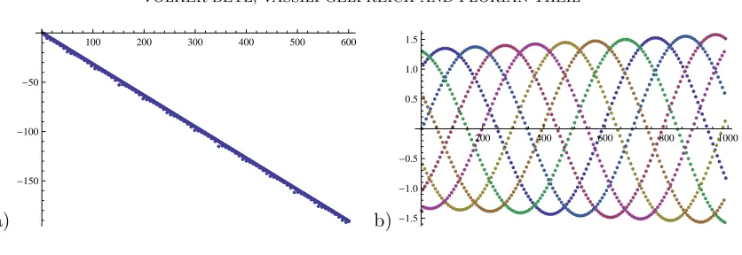
Surprisingly,Snconverges to zero, and very quickly so: a logarithmic plot (cf. Figure 1a)

shows that this convergence is exponential! But that is not all. By Figure 1a, it appears

that the exponential rate of convergence of Sn is just under 1/3; so we will take a brave

guess and say it is 1/π. Let us cancel this exponential decay and see what we get. Plotting

˜

Sn = (−1)nSnen/π (cf. Figure 1b) makes things appear even more mysterious: now we

2 VOLKER BETZ, VASSILI GELFREICH AND FLORIAN THEIL

a)

100 200 300 400 500 600

-150 -100 -50

b)

200 400 600 800 1000

-1.5 -1.0 -0.5 0.5 1.0 1.5

Figure 1. a) ln_|Sn| for n = 1, . . . ,600. b) The first 1000 values of

(₋1)n_S

nen/π, coloured modulo seven.

not only have a sequence that has no reason to converge, but nevertheless does, but when the exponential decay rate is taken out, it displays a complicated and rather beautiful

structure: There are seven sine curves hidden in the values of ˜Sn, each of them with a

period of just under 700, and a very slight overall increase in amplitude. (The factor (₋1)n

is there for cosmetic reasons: without it, we would see not seven but fourteen sine curves, in pairs such that for every curve the negative curve is also present. The image would not look nearly as nice.)

These images make the second question about the reason for the behaviour ofSnall the

more interesting. In addition, further questions arise: why is the re-normalized sequence

displaying a beautiful pattern of interlaced sine curves? What have the numbers 1/π and

7 to do with it?

In the case of (1), we will be able to answer all these questions analytically, and by

doing it find a very good (but hidden) reason for Sn to converge. Before doing this, let

us see whether (1) is an isolated freak phenomenon, or whether there are more of those sequences that converge without having any obvious reason to do so.

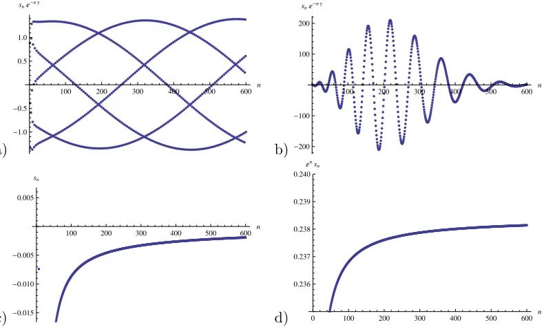
It turns out that there are many, and we have listed some of those that we found in Table 1. Let us call them oscillatory sums, for their formal similarity with oscillatory

integrals. Not all oscillatory sums converge, but all seem to be much _{smaller than their}

maximal element, or even the difference between the maximal element and the next smaller one. Also, some oscillatory sums show the interlaced sine curves when re-normalized, while some do not, see Figure 2. There are many oscillatory sums where no analytic trick like the one that we will use to treat (1) seems to work, but which nonetheless behave in a very regular way. At present, we have no idea how general this behaviour is. Have we maybe unconsciously picked sequences that are similar enough to (1) in order to behave similarly? Also, we do not know whether there is a common reason for all of them to behave as they do, or whether one has to study them case by case. It is essentially only in the case of (1) that we have a good idea of what is going on, which we will now present.

Let us view Sn not as a sequence, but as the valuesf(n) that some function f attains

at the integers. We define

f(t) =

⌊t⌋ X k=0

(k₋t)k

k! , (t >0) (2)

where _⌊t_⌋ denotes the integer part of t _∈R_{. For t < 0 we set f(t) = 0. The function f}

sn max elem_{(n= 600)} ∆ max elem_{(n= 600)} |s600| exponential_{rate γ} graph

n X k=0

(k2_−n2₎k

(2k)! 1.8×10

235 _9.6×10232 _1.0×1033 _{0.1266 Fig. 2 a)}

n X k=0

(k2₋n2)k

(3k)! 3.5×10

29 _5.0×1026 _6.5×1014 _{(0.0569) Fig. 2 b)}

n X k=0

(√k₋√n)k

k! 5.1×10

7 _9.1×105 _1.9×10−3 _{0 Fig. 2 c)}

2n X k=0

e−n1(k−n)2(−1)k 1 1.6×10−3 6.3×10−262 −1 Fig. 2 d)

Table 1. Four oscillatory sums: max elem denotes the element of maximal absolute value, ∆ max elem the difference between the abslolute values of

the latter and the next smaller one, taken atn= 600. The exponential rate

of growth or decay is estimated from the numerics; the value in brackets indicates that in this case, the growth is not actually exponential.

a)

100 200 300 400 500 600 n

-1.0 -0.5 0.5 1.0 snã-nΓ

b)

100 200 300 400 500 600 n

-200 -100 100 200

snã-nΓ

c)

100 200 300 400 500 600 n

-0.015 -0.010 -0.005 0.005 sn

d) 0 100 200 300 400 500 600 n

0.236 0.237 0.238 0.239 0.240 ãnsn

Figure 2. Plots of the renormalized oscillatory sums from Table 1. We

plottedsne−γn forn= 1, . . . ,600, whereγ is the exponential rate given in

the next to last column of Table 1.

polynomial, being a polynomial of degreenin the interval [n, n+ 1]. f is differentiable on

(1,_∞), more preciselyf _∈Cn_{(n,∞) for anyn∈N. To see this, note that whentincreases}

and crosses an integer value n _∈ N_{, the sum in the definition of f gains the additional}

4 VOLKER BETZ, VASSILI GELFREICH AND FLORIAN THEIL

But most importantly,f is the unique solution of the equation 1)

f′(t) =₋f(t₋1) (t /_{∈ {}0,1_}) (3) subject to the initial condition

f(t) = 1 fort_∈[0,1].

Indeed, if t_6∈Nwe can differentiate the definition of f to obtain

f′(t) =₋

⌊t⌋ X k=1

(k₋t)k−1

(k₋1)! =−

⌊t−1⌋ X k=0

(k+ 1₋t)k

k! =−f(t−1).

For integer t _≥ 2, the equation follows from the continuity of f and f′. Existence of a

unique solution to (3) follows from considering the integral form of the equation,

f(t) = 1₋

Z t−1

0

f(s)ds,

fort_≥1: existence is obtained by induction on the intervals [n, n+ 1], and for uniqueness

note that the differenceg(t) of two solutions satisfies_|g(t)_|6 R₀t−1_|g(s)_|ds,g(0) = 0, and apply the Gronwall lemma. By a similar argument, or by a direct estimate on (2), we can see that f(t)6 et for allt>0.

So f satisfies a linear delay-differential equation with constant coefficients, which can

be solved using the Laplace transform. Let

u(p) =

Z ∞

0

e−ptf(t)dt

be the Laplace transform of f. Since we have just seen that f(t) 6 et, the integral is

finite at least for Re (p) >1. In order to derive the equation for u we multiply equation

(3) bye−pt and integrate from 1 to _∞. Integrating the left hand side by parts we obtain

Z ∞

1

e−ptf′(t)dt = ₋e−pf(1) +p Z ∞

1

e−ptf(t)dt

= ₋e−p₋p

Z 1

0

e−ptdt+pu(p) =₋1 +pu(p).

Integrating the right hand side we get

Z ∞

1

e−ptf(t₋1)dt =

Z ∞

0

e−p(t+1)f(t)dt=e−pu(p).

Therefore

−1 +pu(p) =₋e−pu(p) and consequently

u(p) = 1

p+ e−p .

To get back to the function f, we need to invert the Laplace transform. For this, let us

first study the analytic continuationu(z) ofu. It has simple poles where the denominator

is zero, i.e. where

z+ e−z = 0, (4)

and it is analytic otherwise. Since (4) is equivalent to zez = ₋1, the poles closest to

the real axis are W(₋1) and W(₋1), where W is the Lambert function, i.e. the inverse

function of zez. This function is multi-valued, and in order to get error estimates, we want the location of the next pair of poles, too.

We transform (4) into the pair of real equations

−x = e−x cosy (5)

y = e−x siny , (6)

with z=x+ iy. Since f is real on the real line, singularities come in complex conjugate

pairs, and we restrict to y > 0. Equation (6) implies that ex _{= sin(y)/y 61, so x <0,}

which means that all the singularities are on the left of the real axis. Squaring and adding

(5) and (6) yields y2 _{= e}−2x _−x2_{, so for any solution |y|grows monotonically with |x|,}

and vice versa. Finally, rearranging (6) and taking the logarithm yields x = ln(sin(y)/y)

whenever sin(y)>0, with no real solution otherwise. Inserted into (5), this leads to

ln(sin_yy) siny=₋ycosy. (7)

The left hand side of (7) is defined for (kπ,(k+ 1)π) with k even, and has exactly one

solution in each of these intervals. The first two of them arey1 = 1.33724 andy2= 7.58863,

leading to z1 =W(−1)≈ −0.31832 + 1.33724i and z2 ≈ −2.06228 + 7.58863i. All further

solutions have even larger negative real part.

The inverse Laplace transform can now be done using the Bromwich integral:

f(t) = 1 2πi

Z i∞ −i∞

ept p+e−pdp ,

where as a path of integration we choose the imaginary axis, which is right of all

singu-larities of u, as is required. Now, shifting the path of integration to the left and using

residues, we get

f(t) = 2Re e

z1t

1 +z1

+O( e−Re (z2)t_).

Withzj =xj+ iyj this gives

f(t) = 2 |1 +z1|

ex1t _cos(y

1t+ arg(1 +z1)) +O(ex2t). (8)

So, f is a decaying exponential times a cosine function, and we are in the position to

answer all of the questions that we asked before. Firstly, what does 1/π have to do with

Sn? The answer is, nothing at all, except that it happens to agree with the−Re (W(−1))

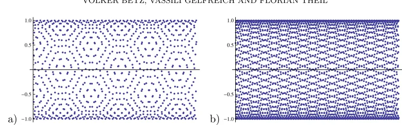
in the first four valid digits. The discrepancy is small enough so it does not lead to an exponential growth in Figure 1b, although a slight increase of amplitude is indeed visible. Secondly, what has seven to do with it, and why do we see the interlaced sine functions? Given (8), the answer becomes obvious, although it may have been obvious form the start for people who are working in signal processing. Have a look at Figures 3a and 3b, and guess what you are seeing.

The surprising answer is that both of the plots actually depict the same sequence,

namely (cos(n))n∈N. The only difference is that the first plot contains the first 1000

elements, while the second one contains the first 3000 ones. If you want to verify this, hold Figure 3a in front of your eyes at an acute angle, and look over it from the side! Apart from telling us that we might want to be careful when drawing conclusions from looking at plots, Figure 3b could have suggested from the start what we have seen in (8),

namely that Sn is an undersampling of a trigonometric function at a frequency that is

6 VOLKER BETZ, VASSILI GELFREICH AND FLORIAN THEIL

a) -1.0 -0.5 0.5 1.0

b)-1.0 -0.5 0.5 1.0

Figure 3. Guess what sequence you are seeing in each of these pictures!

7 (or rather 14, as discussed above) for Sn is not hard to understand any more: If we

consider the defect of diophantine approximations

d(n) = min

16p,q6n

Im (z1)

2π −

p q ,

then the numbersnwheredjumps correspond to sampling frequencies which will give the

illusion of periodic behavior. If N points are plotted then we need that N d(n) = O(1).

The first solution for 1000d(n)63 is obtained forn= 14.

Let us finally note that the trick of writing an oscillatory sum as the values of a function at integer points, and deriving a differential equation for that function, works for a few other sums: e.g., for the truncated negative exponentialsn(γ) =P⌊γn⌋_k=0(−n)k/k!, withγ >

0, we introduces(t) =P⌊γt⌋

k=0(−t)k/k! and obtain the equations′(t)+s(t) = (−t)⌊γt⌋/⌊γt⌋!,

with the solution

s(t) = e−t1 +

Z t

0

er (−r)

⌊γr⌋

⌊γr_⌋! dr

. (9)

A simple estimate of the integrand using Stirling’s formula shows thats(t) diverges when

γ <e, decays exponentially but not as quickly as e−t _{when e< γ < 1/W(1/e) ≈3.591}

(with W again the Lambert function); in the latter case the integral in (9) still diverges.

For γ > 1/W(1/e), s(t) converges like e−t. We could have had the same insight by

estimating the first remainder term nγn_{/(γn)!. On the other hand, a sum of the form}

sn = P⌊n/α⌋_k=0 β

k (αk−n)k

k! , when transformed to a function s(t) in the obvious way, fulfills

s′_{(t) = −βs(t−α) for every α, β > 0, and can be treated in the same way as S}

n. But

this seems to be pretty much the furthest we can stretch the idea of solving a simple differential equation to treat an oscillatory sum: in particular, we re-emphasize that for the many types of oscillatory sums that we tried, including those in Table 1, we have found no way of understanding the highly regular behaviour they seem to exhibit.

Volker Betz, Vassili Gelfreich, Florian Theil Department of Mathematics