Date Name Dept. Title Prepared 2016-05-31 Stefan Klooster PG DR TE PDT HGO
SGT-600 Lube Oil System Simulation
Matlab Simulink ModelChecked 2016-05-31 Geert de Boer PG DR TE PDT HGO
T
ra
n
s
m
itta
l, r
e
p
ro
d
u
ctio
n
,
d
isse
m
ina
tio
n
a
n
d
/o
r e
d
iting
o
f
th
is d
o
c
u
m
e
n
t
a
s
well a
s u
tili
za
tio
n
o
f
its c
o
n
te
n
ts
a
n
d
co
m
m
u
n
ica
tio
n
t
h
e
re
o
f
to
o
th
e
rs
wi
th
o
u
t
e
xp
re
ss a
u
th
o
rizat
ion
a
re
p
ro
h
ibite
d
.
Of
fe
n
d
e
rs
wil
l b
e
h
e
ld
lia
b
le
f
o
r
p
a
ym
e
n
t
o
f
d
a
m
a
g
e
s.
A
ll r
igh
ts
cr
e
a
te
d
b
y p
a
te
n
t
g
ra
n
t
o
r
re
g
istr
a
tio
n
o
f a
u
tili
ty
m
o
d
e
l o
r d
e
sign
p
a
te
n
t a
re
r
e
se
rv
e
d
.
SGT-600 Lube Oil System Simulation
Matlab Simulink Model
Name: Stefan Klooster Student number: s1196782
Company: Siemens Nederland N.V. Department: Technology & Innovation Project Coordinator: G. de Boer
Hengelo, The Netherlands March 1st till May 31st 2016.
T
ra
n
s
m
itta
l, r
e
p
ro
d
u
ctio
n
,
d
isse
m
ina
tio
n
a
n
d
/o
r e
d
iting
o
f
th
is d
o
c
u
m
e
n
t
a
s
well a
s u
tili
za
tio
n
o
f
its c
o
n
te
n
ts
a
n
d
co
m
m
u
n
ica
tio
n
t
h
e
re
o
f
to
o
th
e
rs
wi
th
o
u
t
e
xp
re
ss a
u
th
o
rizat
ion
a
re
p
ro
h
ibite
d
.
Of
fe
n
d
e
rs
wil
l b
e
h
e
ld
lia
b
le
f
o
r
p
a
ym
e
n
t
o
f
d
a
m
a
g
e
s.
A
ll r
igh
ts
cr
e
a
te
d
b
y p
a
te
n
t
g
ra
n
t
o
r
re
g
istr
a
tio
n
o
f a
u
tili
ty
m
o
d
e
l o
r d
e
sign
p
a
te
n
t a
re
r
e
se
rv
e
d
.
SGT-600 Lube Oil System Simulation
Matlab Simulink Model
Classification
RESTRICTED
Client
Internal
Project Title
SGT600 Lube Oil System
Project Number
ZIA-723 SPA08 SP04 WP17
T
ra
n
s
m
itta
l, r
e
p
ro
d
u
ctio
n
,
d
isse
m
ina
tio
n
a
n
d
/o
r e
d
iting
o
f
th
is d
o
c
u
m
e
n
t
a
s
well a
s u
tili
za
tio
n
o
f
its c
o
n
te
n
ts
a
n
d
co
m
m
u
n
ica
tio
n
t
h
e
re
o
f
to
o
th
e
rs
wi
th
o
u
t
e
xp
re
ss a
u
th
o
rizat
ion
a
re
p
ro
h
ibite
d
.
Of
fe
n
d
e
rs
wil
l b
e
h
e
ld
lia
b
le
f
o
r
p
a
ym
e
n
t
o
f
d
a
m
a
g
e
s.
A
ll r
igh
ts
cr
e
a
te
d
b
y p
a
te
n
t
g
ra
n
t
o
r
re
g
istr
a
tio
n
o
f a
u
tili
ty
m
o
d
e
l o
r d
e
sign
p
a
te
n
t a
re
r
e
se
rv
e
d
.
Stefan Klooster s1196782
Siemens Nederland N.V. Energy Sector Oil & Gas Industrieplein 3
7553 LL Hengelo The Netherlands
Department: Technology & Innovation
Department Manager: M. Buse, [email protected] Phone +31 (0) 74 2402562 Mobile +31(0)6 12026270
Project Coordinator: G. de Boer, [email protected] Phone +31 (0) 74 240 2397
March 1st till May 31st 2016.
T
ra
n
s
m
itta
l, r
e
p
ro
d
u
ctio
n
,
d
isse
m
ina
tio
n
a
n
d
/o
r e
d
iting
o
f
th
is d
o
c
u
m
e
n
t
a
s
well a
s u
tili
za
tio
n
o
f
its c
o
n
te
n
ts
a
n
d
co
m
m
u
n
ica
tio
n
t
h
e
re
o
f
to
o
th
e
rs
wi
th
o
u
t
e
xp
re
ss a
u
th
o
rizat
ion
a
re
p
ro
h
ibite
d
.
Of
fe
n
d
e
rs
wil
l b
e
h
e
ld
lia
b
le
f
o
r
p
a
ym
e
n
t
o
f
d
a
m
a
g
e
s.
A
ll r
igh
ts
cr
e
a
te
d
b
y p
a
te
n
t
g
ra
n
t
o
r
re
g
istr
a
tio
n
o
f a
u
tili
ty
m
o
d
e
l o
r d
e
sign
p
a
te
n
t a
re
r
e
se
rv
e
d
.
TABLE OF CONTENTS
Executive Summary ... 6
Nomenclature... 7
1 Introduction ... 8
2 System description ... 9
3 Assignment description ... 10
4 Simulation model ... 11
4.1 General assumptions ... 11
4.2 Iterative model ... 12
4.2.1 Centrifugal pump ... 12
4.2.2 Orifice plate ... 13
4.2.3 Iterative scheme ... 13
4.3 Integration model ... 14
4.3.1 Electric motor ... 15
4.3.2 Centrifugal pump ... 16
4.3.3 Result Integration model ... 18
4.4 Total model ... 19
4.4.1 Model extension ... 19
4.4.2 Parallel flow ... 20
4.4.3 Flow feedback ... 20
4.4.4 Conditions ... 20
5 Final model ... 22
5.1 Pipe pressure loss ... 23
5.2 Cooler ... 25
5.3 3 way temperature valve ... 25
5.4 Filter ... 25
5.5 Gas Turbine bearings ... 25
5.6 Compressor bearings ... 26
5.7 Gear ... 26
5.8 Viscosity ... 26
5.9 Static head ... 27
5.10 Bypass orifice ... 28
6 Results ... 29
T
ra
n
s
m
itta
l, r
e
p
ro
d
u
ctio
n
,
d
isse
m
ina
tio
n
a
n
d
/o
r e
d
iting
o
f
th
is d
o
c
u
m
e
n
t
a
s
well a
s u
tili
za
tio
n
o
f
its c
o
n
te
n
ts
a
n
d
co
m
m
u
n
ica
tio
n
t
h
e
re
o
f
to
o
th
e
rs
wi
th
o
u
t
e
xp
re
ss a
u
th
o
rizat
ion
a
re
p
ro
h
ibite
d
.
Of
fe
n
d
e
rs
wil
l b
e
h
e
ld
lia
b
le
f
o
r
p
a
ym
e
n
t
o
f
d
a
m
a
g
e
s.
A
ll r
igh
ts
cr
e
a
te
d
b
y p
a
te
n
t
g
ra
n
t
o
r
re
g
istr
a
tio
n
o
f a
u
tili
ty
m
o
d
e
l o
r d
e
sign
p
a
te
n
t a
re
r
e
se
rv
e
d
.
6.2 Bypass orifice diameter ... 29
6.3 Torque ... 31
6.4 Flow-head curves... 32
6.5 Parallel flows ... 33
6.6 Compressor bearings ... 34
7 Conclusion ... 35
8 Recommendations ... 36
9 List of references ... 37
10 Reference documents... 38
Attachment 1: Datasheet pumps ... 38
Attachment 2: Centrifugal pumps approximation... 40
Attachment 3: Orifice plate ... 42
Attachment 4: Datasheet electric motor ... 44
T
ra
n
s
m
itta
l, r
e
p
ro
d
u
ctio
n
,
d
isse
m
ina
tio
n
a
n
d
/o
r e
d
iting
o
f
th
is d
o
c
u
m
e
n
t
a
s
well a
s u
tili
za
tio
n
o
f
its c
o
n
te
n
ts
a
n
d
co
m
m
u
n
ica
tio
n
t
h
e
re
o
f
to
o
th
e
rs
wi
th
o
u
t
e
xp
re
ss a
u
th
o
rizat
ion
a
re
p
ro
h
ibite
d
.
Of
fe
n
d
e
rs
wil
l b
e
h
e
ld
lia
b
le
f
o
r
p
a
ym
e
n
t
o
f
d
a
m
a
g
e
s.
A
ll r
igh
ts
cr
e
a
te
d
b
y p
a
te
n
t
g
ra
n
t
o
r
re
g
istr
a
tio
n
o
f a
u
tili
ty
m
o
d
e
l o
r d
e
sign
p
a
te
n
t a
re
r
e
se
rv
e
d
.
Executive Summary
The lube oil system in the SGT 600 has to supply oil of the correct pressure and temperature to the gas turbine bearings, the gear and the compressor bearings for lubrication and cooling. The
lubrication oil used in the system is mineral based turbine oil ISO VG 46. The oil in the system goes through multiple components before the bearings and gear are reached. Two centrifugal pumps, which are driven by electric motors, pump the oil through a cooler, bypass line, 3 way temperature valve and a filter before the oil enters the bearings. All these components have a pressure loss (resistance) which depends on the flow that goes through the component. On the other side, the flow that is present in the system depends on the resistance of the total system.
To show this dynamic behaviour of the system, a simplified mathematical simulation model is required for the start-up of the lube oil system of the SGT 600. This model must calculate the flow and pressure in each part of the lube oil system. Furthermore, the bypass line over the cooler has an orifice plate which must take care of a pressure loss that is equal to the pressure drop of the cooler. The simulation model must provide a suitable selection tool for the orifice bore diameter of the bypass line.
The simulation tool used for this model is Matlab Simulink. To simulate the total lube oil system, the model is split into an iterative part and an integration part. For the total model, these two parts are coupled after both models are tested. The iterative part finds the flow in the total lube oil system and the integration part takes care of the coupling between the electric motors and the centrifugal pumps. This way, the start-up behaviour can be described.
From available datasheets it can be seen that the desired pressure upstream the bearings in the system does not correspond to the design flow and speed of the centrifugal pumps. So the
centrifugal pumps do not operate at their best efficiency point. The simulation tool described in this report will predict the flow and the pressure at every component in the system.
The final model described in this report is capable of finding the pressure and flow at each
component in the system. However, the final model contains a lot of assumptions which cannot be validated due to a lack of data. Also, the model is capable of showing the physical behaviour. This physical behaviour contains the distribution of the flow over parallel components, where the components with the lowest resistance gets the most flow. It also contains the dynamic behaviour where the resistance determines the flow in the system and the flow on its turn determines the resistance.
T
ra
n
s
m
itta
l, r
e
p
ro
d
u
ctio
n
,
d
isse
m
ina
tio
n
a
n
d
/o
r e
d
iting
o
f
th
is d
o
c
u
m
e
n
t
a
s
well a
s u
tili
za
tio
n
o
f
its c
o
n
te
n
ts
a
n
d
co
m
m
u
n
ica
tio
n
t
h
e
re
o
f
to
o
th
e
rs
wi
th
o
u
t
e
xp
re
ss a
u
th
o
rizat
ion
a
re
p
ro
h
ibite
d
.
Of
fe
n
d
e
rs
wil
l b
e
h
e
ld
lia
b
le
f
o
r
p
a
ym
e
n
t
o
f
d
a
m
a
g
e
s.
A
ll r
igh
ts
cr
e
a
te
d
b
y p
a
te
n
t
g
ra
n
t
o
r
re
g
istr
a
tio
n
o
f a
u
tili
ty
m
o
d
e
l o
r d
e
sign
p
a
te
n
t a
re
r
e
se
rv
e
d
.
Nomenclature
Symbol
Description
Unit
𝛽 Ratio of orifice hole diameter to pipe diameter [-]
𝜖 Relative eccenctricity, 𝜖 = 𝑒/𝑟 [-]
𝜖𝑟 Roughness [𝑚𝑚]
𝜂 Efficiency [-]
𝜇 Dynamic viscosity [𝑘𝑔/𝑚𝑠]
𝜔 Angular velocity [1/𝑠]
𝜌 Density [𝑘𝑔/𝑚3]
𝐴𝑜𝑟𝑖𝑓 Cross sectional area orifice hole [𝑚2]
𝐶 Flow coefficient [-]
𝑐 Radial clearance at neutral position [𝑚]
𝐶𝑑 Discharge coefficient [-]
𝑑 Diameter orifice hole [𝑚]
𝐷 Pipe diameter [𝑚]
𝑓𝐷 Darcy-Weisbach friction factor [-]
𝑔 Gravitational acceleration [𝑚/𝑠2]
ℎ Head pressure [𝑚]
ℎ𝑑 Design head pressure [𝑚]
ℎ𝑠𝑜 Shut-off head pressure [𝑚]
ℎ𝑠𝑡𝑎𝑡 Static head pressure [𝑚]
𝐽 Moment of inertia [𝑘𝑔𝑚2]
𝑙 Length of the half-bearing [𝑚]
𝐿 Pipe length [𝑚]
𝑁 Speed [𝑅𝑃𝑀]
𝑝 Pressure [𝑃𝑎]
𝑝1 Pressure upstream orifice [𝑃𝑎]
𝑝2 Pressure downstream orifice [𝑃𝑎]
𝑃ℎ Hydraulic power [𝑊]
𝑃𝑚𝑜𝑡𝑜𝑟 Power of electric motor [𝑊]
𝑃𝑠 Shaft power [𝑊]
𝑄 Volume flow [𝑚3/𝑠 ]
𝑄
𝑑Design flow
[
𝑚
3/𝑠
]
𝑟 Ratio between max and design flow [-]
𝑟 Journal radius [𝑚]
𝑅𝑒 Reynolds number [-]
𝑠 Stable flow range [-]
𝑡 Time [𝑠]
𝑇 Torque [𝑁𝑚]
𝑇𝑚𝑜𝑡𝑜𝑟 Torque delivered by electric motor [𝑁𝑚]
𝑇𝑝𝑢𝑚𝑝 Torque required by pump [𝑁𝑚]
T
ra
n
s
m
itta
l, r
e
p
ro
d
u
ctio
n
,
d
isse
m
ina
tio
n
a
n
d
/o
r e
d
iting
o
f
th
is d
o
c
u
m
e
n
t
a
s
well a
s u
tili
za
tio
n
o
f
its c
o
n
te
n
ts
a
n
d
co
m
m
u
n
ica
tio
n
t
h
e
re
o
f
to
o
th
e
rs
wi
th
o
u
t
e
xp
re
ss a
u
th
o
rizat
ion
a
re
p
ro
h
ibite
d
.
Of
fe
n
d
e
rs
wil
l b
e
h
e
ld
lia
b
le
f
o
r
p
a
ym
e
n
t
o
f
d
a
m
a
g
e
s.
A
ll r
igh
ts
cr
e
a
te
d
b
y p
a
te
n
t
g
ra
n
t
o
r
re
g
istr
a
tio
n
o
f a
u
tili
ty
m
o
d
e
l o
r d
e
sign
p
a
te
n
t a
re
r
e
se
rv
e
d
.
1
Introduction
The Siemens SGT-600 is a heavy-duty industrial gas turbine designed and built to meet requirements for low life-cycle cost. The lube oil system in the SGT 600 has to supply oil of the correct pressure and temperature to the gas turbine bearings, the gear and the compressor bearings for lubrication and cooling.
A simulation model is required for the start-up of the lube oil system of the SGT 600. This model must calculate the flow and pressure in each part of the lube oil system during start-up. The simulation tool used for this model is Matlab Simulink. To simulate the total lube oil system, the model is split into two parts and these are coupled after both models are tested.
The first model is an iterative model, which finds the flow in a system with centrifugal pumps and an orifice plate, which sets the resistance in the system. This iterative model is described in section 4.2. The second model is an integration model, which is describe in section 4.3. This model couples the electric motor to the centrifugal pumps. Due to the torque delivered by the electric motors, the pumps accelerate. They will accelerate until the delivered torque is equal to the required torque by the pumps.
The two models described above are coupled to each other, which is described in section 4.4. Due to this coupling, the start-up of the lube oil system can be simulated. After this coupling is made, the system is extended towards the final model.
The final model contains the components which are present in the real system. These components all have a pressure loss (resistance) which depends on the flow that goes through the component. At the same time, the flow that goes through the system depends on the resistance of the system. The final model has the goal to find the flow and pressure everywhere in the system. The final model is described in chapter 5.
T
ra
n
s
m
itta
l, r
e
p
ro
d
u
ctio
n
,
d
isse
m
ina
tio
n
a
n
d
/o
r e
d
iting
o
f
th
is d
o
c
u
m
e
n
t
a
s
well a
s u
tili
za
tio
n
o
f
its c
o
n
te
n
ts
a
n
d
co
m
m
u
n
ica
tio
n
t
h
e
re
o
f
to
o
th
e
rs
wi
th
o
u
t
e
xp
re
ss a
u
th
o
rizat
ion
a
re
p
ro
h
ibite
d
.
Of
fe
n
d
e
rs
wil
l b
e
h
e
ld
lia
b
le
f
o
r
p
a
ym
e
n
t
o
f
d
a
m
a
g
e
s.
A
ll r
igh
ts
cr
e
a
te
d
b
y p
a
te
n
t
g
ra
n
t
o
r
re
g
istr
a
tio
n
o
f a
u
tili
ty
m
o
d
e
l o
r d
e
sign
p
a
te
n
t a
re
r
e
se
rv
e
d
.
2
System description
The lube oil system in the SGT 600 has to supply oil of the correct pressure and temperature to the gas turbine bearings, the gear and the compressor bearings for lubrication and cooling. The lubrication oil used in the system is mineral based turbine oil ISO VG 46. In Figure 1, a simplified Piping and Instrumentation Diagram (P&ID) is shown. It can be seen that the lube oil system starts at the lube oil tank. In this tank, three centrifugal pumps are installed. These pumps are driven by three electric motors. In normal operation, two pumps work at 50%, and the third is in standby mode. After the pumps, a part of the oil goes through a cooler and the other part of the flow goes through a bypass line. This bypass line has an orifice plate, which is responsible for a pressure loss which must be the same as the pressure loss over the cooler. The flow through the cooler and the bypass are combined in the three way temperature valve. The function of this valve is to ensure a set temperature and regulate the flows over the bypass line and the cooler. This valve uses the
temperature of the incoming flows to regulate the flow over the cooler and the bypass. After the three way temperature valve, the oil goes through a duplex filter. After the filter, the flow is split; a part goes to the gas turbine bearings, the gear and the compressor bearings. The other part of the flow goes into high pressure (positive displacement) pumps. The high pressure pumps deliver oil to the high pressure bearing of the gas turbine. After the oil lubricated the bearings and the gear, the oil flows back into the oil tank through drains.
T
ra
n
s
m
itta
l, r
e
p
ro
d
u
ctio
n
,
d
isse
m
ina
tio
n
a
n
d
/o
r e
d
iting
o
f
th
is d
o
c
u
m
e
n
t
a
s
well a
s u
tili
za
tio
n
o
f
its c
o
n
te
n
ts
a
n
d
co
m
m
u
n
ica
tio
n
t
h
e
re
o
f
to
o
th
e
rs
wi
th
o
u
t
e
xp
re
ss a
u
th
o
rizat
ion
a
re
p
ro
h
ibite
d
.
Of
fe
n
d
e
rs
wil
l b
e
h
e
ld
lia
b
le
f
o
r
p
a
ym
e
n
t
o
f
d
a
m
a
g
e
s.
A
ll r
igh
ts
cr
e
a
te
d
b
y p
a
te
n
t
g
ra
n
t
o
r
re
g
istr
a
tio
n
o
f a
u
tili
ty
m
o
d
e
l o
r d
e
sign
p
a
te
n
t a
re
r
e
se
rv
e
d
.
3
Assignment description
A simplified mathematical model of the system is required representing the physical behaviour of the lube oil system. Suitable assumptions have to be included representing the several components in the system and in particular the oil characteristics. To simulate the dynamic response of the system, the equations need to be solved using Matlab Simulink.
T
ra
n
s
m
itta
l, r
e
p
ro
d
u
ctio
n
,
d
isse
m
ina
tio
n
a
n
d
/o
r e
d
iting
o
f
th
is d
o
c
u
m
e
n
t
a
s
well a
s u
tili
za
tio
n
o
f
its c
o
n
te
n
ts
a
n
d
co
m
m
u
n
ica
tio
n
t
h
e
re
o
f
to
o
th
e
rs
wi
th
o
u
t
e
xp
re
ss a
u
th
o
rizat
ion
a
re
p
ro
h
ibite
d
.
Of
fe
n
d
e
rs
wil
l b
e
h
e
ld
lia
b
le
f
o
r
p
a
ym
e
n
t
o
f
d
a
m
a
g
e
s.
A
ll r
igh
ts
cr
e
a
te
d
b
y p
a
te
n
t
g
ra
n
t
o
r
re
g
istr
a
tio
n
o
f a
u
tili
ty
m
o
d
e
l o
r d
e
sign
p
a
te
n
t a
re
r
e
se
rv
e
d
.
4
Simulation model
To simulate the lube oil system, first some assumptions have to be made in order to get a clear vision of what has to be simulated. This is done in section 4.1. After these assumptions, in section 4.2, an iterative model is explained in which the operating point of an centrifugal pump is found at a constant speed. Then an integration model is described in section 4.3. This model is used to simulate the start-up of the pumps, which are driven by electric motors. These models are then coupled and extended in section 4.4 in order to simulate the complete lube oil system.
4.1
General assumptionsThe simulation model has to find the flow in the system together with the resistance in the system. Assumptions made for this model are:
The resistance in the system will also be affected by temperature changes in the system, because the viscosity is dependent on the temperature. However, for all the models in this report, a constant temperature is assumed during start-up of the lube oil system. This is done because the total time for start-up is relatively short and only a small amount of the total oil will be heated during the start-up, so the bulk temperature in the oil tank will hardly change.
It is also assumed that oil is present everywhere in the system when the system is started. This has the consequence that a pressure difference in the system directly leads to a flow. So the model is not sequential, where the flow would start in the pumps and move through the system.
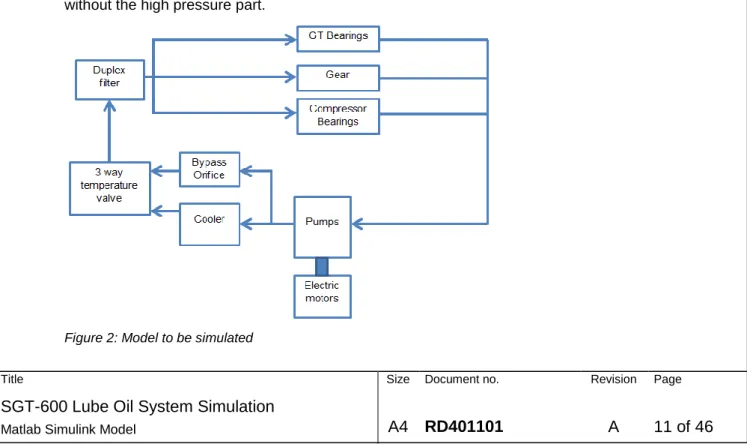
The high pressure part of the lube oil system is not taken into account for the simulation model. This is done because this is a separate loop, which has not much effect on the rest of the system. The high pressure bearing is simulated as a normal gas turbine bearing.
The lube oil system that is eventually going to be simulated in this report is shown in Figure 2, so without the high pressure part.
T
ra
n
s
m
itta
l, r
e
p
ro
d
u
ctio
n
,
d
isse
m
ina
tio
n
a
n
d
/o
r e
d
iting
o
f
th
is d
o
c
u
m
e
n
t
a
s
well a
s u
tili
za
tio
n
o
f
its c
o
n
te
n
ts
a
n
d
co
m
m
u
n
ica
tio
n
t
h
e
re
o
f
to
o
th
e
rs
wi
th
o
u
t
e
xp
re
ss a
u
th
o
rizat
ion
a
re
p
ro
h
ibite
d
.
Of
fe
n
d
e
rs
wil
l b
e
h
e
ld
lia
b
le
f
o
r
p
a
ym
e
n
t
o
f
d
a
m
a
g
e
s.
A
ll r
igh
ts
cr
e
a
te
d
b
y p
a
te
n
t
g
ra
n
t
o
r
re
g
istr
a
tio
n
o
f a
u
tili
ty
m
o
d
e
l o
r d
e
sign
p
a
te
n
t a
re
r
e
se
rv
e
d
.
4.2
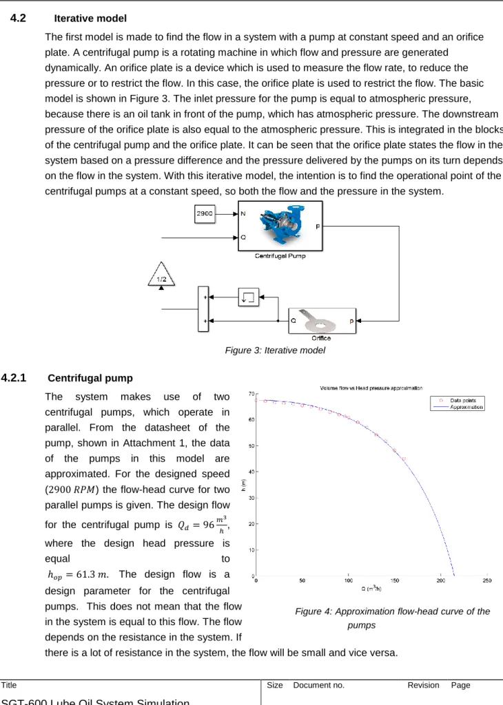
Iterative modelThe first model is made to find the flow in a system with a pump at constant speed and an orifice plate. A centrifugal pump is a rotating machine in which flow and pressure are generated
dynamically. An orifice plate is a device which is used to measure the flow rate, to reduce the pressure or to restrict the flow. In this case, the orifice plate is used to restrict the flow. The basic model is shown in Figure 3. The inlet pressure for the pump is equal to atmospheric pressure, because there is an oil tank in front of the pump, which has atmospheric pressure. The downstream pressure of the orifice plate is also equal to the atmospheric pressure. This is integrated in the blocks of the centrifugal pump and the orifice plate. It can be seen that the orifice plate states the flow in the system based on a pressure difference and the pressure delivered by the pumps on its turn depends on the flow in the system. With this iterative model, the intention is to find the operational point of the centrifugal pumps at a constant speed, so both the flow and the pressure in the system.
Figure 3: Iterative model
4.2.1
Centrifugal pumpThe system makes use of two centrifugal pumps, which operate in parallel. From the datasheet of the pump, shown in Attachment 1, the data of the pumps in this model are approximated. For the designed speed (2900 𝑅𝑃𝑀) the flow-head curve for two parallel pumps is given. The design flow
for the centrifugal pump is 𝑄𝑑= 96 𝑚3
ℎ,
where the design head pressure is
equal to
ℎ𝑜𝑝= 61.3 𝑚. The design flow is a
design parameter for the centrifugal pumps. This does not mean that the flow in the system is equal to this flow. The flow depends on the resistance in the system. If
there is a lot of resistance in the system, the flow will be small and vice versa.
T
ra
n
s
m
itta
l, r
e
p
ro
d
u
ctio
n
,
d
isse
m
ina
tio
n
a
n
d
/o
r e
d
iting
o
f
th
is d
o
c
u
m
e
n
t
a
s
well a
s u
tili
za
tio
n
o
f
its c
o
n
te
n
ts
a
n
d
co
m
m
u
n
ica
tio
n
t
h
e
re
o
f
to
o
th
e
rs
wi
th
o
u
t
e
xp
re
ss a
u
th
o
rizat
ion
a
re
p
ro
h
ibite
d
.
Of
fe
n
d
e
rs
wil
l b
e
h
e
ld
lia
b
le
f
o
r
p
a
ym
e
n
t
o
f
d
a
m
a
g
e
s.
A
ll r
igh
ts
cr
e
a
te
d
b
y p
a
te
n
t
g
ra
n
t
o
r
re
g
istr
a
tio
n
o
f a
u
tili
ty
m
o
d
e
l o
r d
e
sign
p
a
te
n
t a
re
r
e
se
rv
e
d
.
For the approximation of the flow-head curve of the pump, a method is used which uses the design- and maximum flow and head of the pump. Based on these parameters, the curve for the centrifugal pump is made. In Attachment 2 this method is explained in more detail and the result of the approximation is shown in Figure 4. It can be seen that the approximation intersects all the data points, which were read from the curve in Attachment 2. For the last part of the curve, approximately
above 𝑄 = 165𝑚3
ℎ, no more data points are known. For this part of the curve, the head delivered by
the pump drops to zero, which means that the pump does not increase the pressure anymore. It is undesirable for the pumps to operate in this part of the curve.
From the head pressure delivered by the pump, the pressure in the system can be calculated with [1]:
𝑝 = 𝜌𝑔ℎ
This pressure goes towards the orifice plate, where a pressure-flow relation is used to calculate the flow in the system.
4.2.2
Orifice plateAn orifice plate can regulate the flow in a system. Volume flow rates through an orifice plate can be calculated with the orifice equation [2]:
𝑄 = 𝐶𝐴𝑜𝑟𝑖𝑓√
2(𝑝1− 𝑝2)
𝜌
In this equation, 𝐶 is the flow coefficient. In Attachment 3, this coefficient is described in more detail. The flow is thus calculated with the pressure drop over the orifice. The upstream pressure (𝑝1) is
found from the pumps and the downstream pressure (𝑝2) is atmospheric pressure, since that is
equal to the pressure in the oil tank.
4.2.3
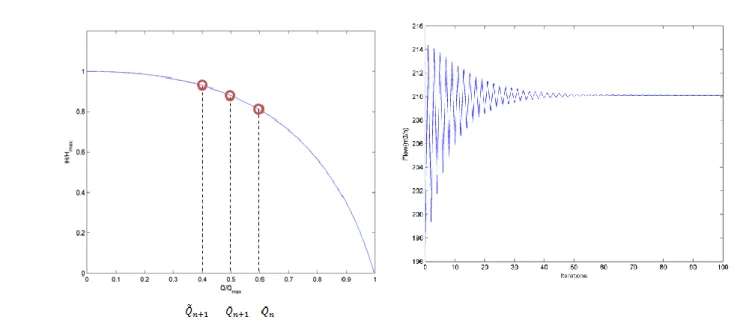
Iterative schemeTo find the operational point of the centrifugal pump, an iterative scheme is used. This is needed because the flow and pressure in the pump are generated dynamically. This is done by giving an initial guess for the flow and correcting the flow with the new computed flow. This is done by adding two successive iterations steps and taking the average of this, which can also be seen in Figure 3. The initial guess is chosen in the memory block in the system. Based on this initial guess, a pressure is calculated in the pumps. When an initial guess for the flow is taken low, the pump will deliver a high head. This will result in a large pressure drop over the orifice plate and thus a large flow. By adding this new flow to the initial guess and averaging it, the flow stays within the boundaries of the pump. At the new calculated large flow, the pump will deliver a low head and this will result in a small flow. Then the circle starts again, where a small flow will result in a high head pressure and thus a large flow. The same will work vice versa, when a too high initial guess is taken too high.
In the method described above, the operational point of the pump is found by moving over the pump curve. This is shown in Figure 5, where 𝑄𝑛 is the initial guess of the flow. 𝑄̃𝑛+1 is the new computed
flow as a consequence of the initial guess and 𝑄𝑛+1 is the average of these two and this is used as a
T
ra
n
s
m
itta
l, r
e
p
ro
d
u
ctio
n
,
d
isse
m
ina
tio
n
a
n
d
/o
r e
d
iting
o
f
th
is d
o
c
u
m
e
n
t
a
s
well a
s u
tili
za
tio
n
o
f
its c
o
n
te
n
ts
a
n
d
co
m
m
u
n
ica
tio
n
t
h
e
re
o
f
to
o
th
e
rs
wi
th
o
u
t
e
xp
re
ss a
u
th
o
rizat
ion
a
re
p
ro
h
ibite
d
.
Of
fe
n
d
e
rs
wil
l b
e
h
e
ld
lia
b
le
f
o
r
p
a
ym
e
n
t
o
f
d
a
m
a
g
e
s.
A
ll r
igh
ts
cr
e
a
te
d
b
y p
a
te
n
t
g
ra
n
t
o
r
re
g
istr
a
tio
n
o
f a
u
tili
ty
m
o
d
e
l o
r d
e
sign
p
a
te
n
t a
re
r
e
se
rv
e
d
.
The number of iterations needed to converge is strongly dependent on the initial guess. As you would expect, the better the initial guess, the less iterations are needed for the same difference in two successive iteration steps.
Figure 5: Finding the operational point of the pumps Figure 6: Converging flow in the system
4.3
Integration modelTo couple the pump and the electric motor, a model is made as shown in Figure 7. The coupling between the two blocks is made with the torque. This coupling takes care of the acceleration of the pump due to the torque that the electric motor delivers. For this model, the input flow for the pumps is a ramp, which starts at zero flow and stops at the design flow; 𝑄𝑑= 96 𝑚3/ℎ.
T
ra
n
s
m
itta
l, r
e
p
ro
d
u
ctio
n
,
d
isse
m
ina
tio
n
a
n
d
/o
r e
d
iting
o
f
th
is d
o
c
u
m
e
n
t
a
s
well a
s u
tili
za
tio
n
o
f
its c
o
n
te
n
ts
a
n
d
co
m
m
u
n
ica
tio
n
t
h
e
re
o
f
to
o
th
e
rs
wi
th
o
u
t
e
xp
re
ss a
u
th
o
rizat
ion
a
re
p
ro
h
ibite
d
.
Of
fe
n
d
e
rs
wil
l b
e
h
e
ld
lia
b
le
f
o
r
p
a
ym
e
n
t
o
f
d
a
m
a
g
e
s.
A
ll r
igh
ts
cr
e
a
te
d
b
y p
a
te
n
t
g
ra
n
t
o
r
re
g
istr
a
tio
n
o
f a
u
tili
ty
m
o
d
e
l o
r d
e
sign
p
a
te
n
t a
re
r
e
se
rv
e
d
.
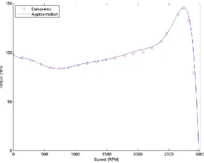
4.3.1
Electric motorThe electric motors used in this model speeds up the centrifugal pumps. How fast the pumps accelerates depends on the requested torque of the pumps and the torque that the electric motors can deliver. The electric motors have a speed-torque relation which is shown in Figure 8. This figure is an approximation of the speed-torque curve in the datasheet, which is given in Attachment 4. In this attachment it can also be seen that the nominal torque of the electric motor is equal to 𝑇𝑛𝑜𝑚=
59 𝑁𝑚 and the speed is equal to 𝑁 = 2971 𝑅𝑃𝑀.
Because two centrifugal pumps, both powered by an electric motor, are present in the total system, the total delivered torque by the electric motor is multiplied by two in the system.
From this curve, the delivered torque at any moment is read at the actual speed. The delivered torque minus the requested torque of the pumps is divided by the moment of inertia of the pumps and the electric motors together. This leads to an angular acceleration for the pumps [3]:
𝑇𝑚𝑜𝑡𝑜𝑟− 𝑇𝑝𝑢𝑚𝑝
𝐽 =
d𝜔 d𝑡
This acceleration is integrated to get the angular velocity of the pumps. The angular velocity can be rewritten to a speed (RPM). When the pump is at a new speed, the pumps do also require more torque. The required torque of the pumps will be explained in section 4.3.2. With the new required torque of the pumps, again an angular velocity is calculated as described above. This leads to acceleration of the pumps until the delivered torque and the required torque are equal. Then a steady state is reached, where the pumps function at a constant speed.
The Simulink model of the electric motor as described above is given in Figure 9. Here, the block T_n_motor contains the speed-torque torque. The speed is the input and the delivered torque is read from the curve.
T
ra
n
s
m
itta
l, r
e
p
ro
d
u
ctio
n
,
d
isse
m
ina
tio
n
a
n
d
/o
r e
d
iting
o
f
th
is d
o
c
u
m
e
n
t
a
s
well a
s u
tili
za
tio
n
o
f
its c
o
n
te
n
ts
a
n
d
co
m
m
u
n
ica
tio
n
t
h
e
re
o
f
to
o
th
e
rs
wi
th
o
u
t
e
xp
re
ss a
u
th
o
rizat
ion
a
re
p
ro
h
ibite
d
.
Of
fe
n
d
e
rs
wil
l b
e
h
e
ld
lia
b
le
f
o
r
p
a
ym
e
n
t
o
f
d
a
m
a
g
e
s.
A
ll r
igh
ts
cr
e
a
te
d
b
y p
a
te
n
t
g
ra
n
t
o
r
re
g
istr
a
tio
n
o
f a
u
tili
ty
m
o
d
e
l o
r d
e
sign
p
a
te
n
t a
re
r
e
se
rv
e
d
.
Figure 9: Simulink model of the electric motor
From the delivered torque and the speed of the electric motor, the power that is delivered by the electric motor can also be calculated [3]:
𝑃𝑚𝑜𝑡𝑜𝑟=
2𝜋 60𝑁𝑇
4.3.2
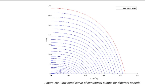
Centrifugal pumpThe centrifugal pump is already described in section 4.2.1. However, this is only for a constant speed. Because the total model is about the start-up of the lube oil system, the flow-head curve of the pumps is scaled with the speed. This is done with the so-called affinity laws. The affinity laws are valid for a constant efficiency, which is assumed for this situation.
The affinity laws state that the flow is proportional to the speed [1]: 𝑄1
𝑄2
=𝑁1 𝑁2
The head pressure is proportional to the square of the speed: ℎ1
ℎ2
= (𝑁1 𝑁2
)
2
T
ra
n
s
m
itta
l, r
e
p
ro
d
u
ctio
n
,
d
isse
m
ina
tio
n
a
n
d
/o
r e
d
iting
o
f
th
is d
o
c
u
m
e
n
t
a
s
well a
s u
tili
za
tio
n
o
f
its c
o
n
te
n
ts
a
n
d
co
m
m
u
n
ica
tio
n
t
h
e
re
o
f
to
o
th
e
rs
wi
th
o
u
t
e
xp
re
ss a
u
th
o
rizat
ion
a
re
p
ro
h
ibite
d
.
Of
fe
n
d
e
rs
wil
l b
e
h
e
ld
lia
b
le
f
o
r
p
a
ym
e
n
t
o
f
d
a
m
a
g
e
s.
A
ll r
igh
ts
cr
e
a
te
d
b
y p
a
te
n
t
g
ra
n
t
o
r
re
g
istr
a
tio
n
o
f a
u
tili
ty
m
o
d
e
l o
r d
e
sign
p
a
te
n
t a
re
r
e
se
rv
e
d
.
Figure 10: Flow-head curve of centrifugal pumps for different speeds
Torque
For the acceleration of the pumps, the required torque of the pumps has to be calculated. This torque depends on the shaft power (𝑃𝑠) and the speed (𝑁)of the pump [4]:
𝑇𝑝𝑢𝑚𝑝=
60 2𝜋
𝑃𝑠
𝑁
The scaling factor is the conversion for rounds per minute to angular velocity. The shaft power is found by the hydraulic power (𝑃ℎ) divided by the efficiency (𝜂) of the pump.
𝑃𝑠=
𝑃ℎ
𝜂
Here, the hydraulic power on its turn can be found with the following formula [4]:
𝑃ℎ =
𝑄𝜌𝑔ℎ 103
Substituting these equations into the equation for the torque, it becomes:
𝑇𝑝𝑢𝑚𝑝=
60 2𝜋
𝑄𝜌𝑔ℎ 𝜂𝑁
Check with data
From the datasheet of the centrifugal pump (see Attachment 1) the torque and power of one centrifugal pump is known at a rotational speed of 𝑛 = 2900 𝑅𝑃𝑀 and a flow of 𝑄 = 48 𝑚3/ℎ. In
Table 1 this data is compared to the data from the model at the same speed and flow. It can be seen that the output of the model corresponds quite good to the datasheet. So the used formulas give the desired output.
Head [m]
Torque [Nm]
Shaft power [kW]
Datasheet
61.3
40.1
12.17
Model
61.3
40.0
12.15
T
ra
n
s
m
itta
l, r
e
p
ro
d
u
ctio
n
,
d
isse
m
ina
tio
n
a
n
d
/o
r e
d
iting
o
f
th
is d
o
c
u
m
e
n
t
a
s
well a
s u
tili
za
tio
n
o
f
its c
o
n
te
n
ts
a
n
d
co
m
m
u
n
ica
tio
n
t
h
e
re
o
f
to
o
th
e
rs
wi
th
o
u
t
e
xp
re
ss a
u
th
o
rizat
ion
a
re
p
ro
h
ibite
d
.
Of
fe
n
d
e
rs
wil
l b
e
h
e
ld
lia
b
le
f
o
r
p
a
ym
e
n
t
o
f
d
a
m
a
g
e
s.
A
ll r
igh
ts
cr
e
a
te
d
b
y p
a
te
n
t
g
ra
n
t
o
r
re
g
istr
a
tio
n
o
f a
u
tili
ty
m
o
d
e
l o
r d
e
sign
p
a
te
n
t a
re
r
e
se
rv
e
d
.
4.3.3
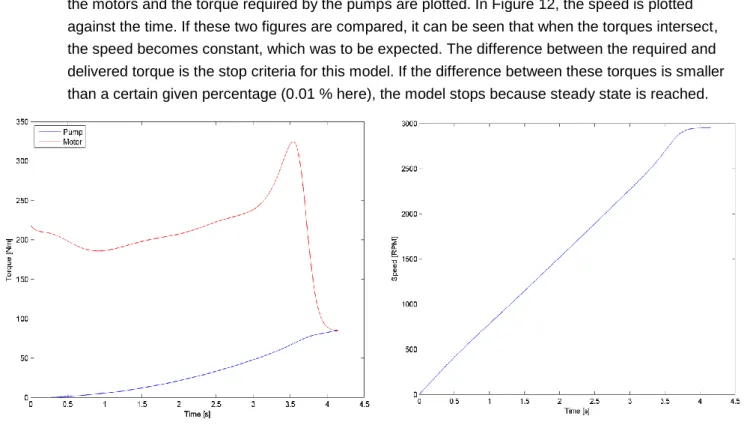
Result Integration modelNow that the torque of both the electric motors and the centrifugal pumps can be related, the centrifugal pumps can be accelerated by the electric motors. In Figure 11, the torque delivered by the motors and the torque required by the pumps are plotted. In Figure 12, the speed is plotted against the time. If these two figures are compared, it can be seen that when the torques intersect, the speed becomes constant, which was to be expected. The difference between the required and delivered torque is the stop criteria for this model. If the difference between these torques is smaller than a certain given percentage (0.01 % here), the model stops because steady state is reached.
Power check
With the equations for the power described above, the power that is required by the pumps and the power that is delivered by the electric motors are calculated. These powers are shown in Figure 13. When the system reaches steady state, the required and delivered power are the same. This shows that no energy is lost in the system.
Figure 11: Torques of the pumps and electric motors
T
ra
n
s
m
itta
l, r
e
p
ro
d
u
ctio
n
,
d
isse
m
ina
tio
n
a
n
d
/o
r e
d
iting
o
f
th
is d
o
c
u
m
e
n
t
a
s
well a
s u
tili
za
tio
n
o
f
its c
o
n
te
n
ts
a
n
d
co
m
m
u
n
ica
tio
n
t
h
e
re
o
f
to
o
th
e
rs
wi
th
o
u
t
e
xp
re
ss a
u
th
o
rizat
ion
a
re
p
ro
h
ibite
d
.
Of
fe
n
d
e
rs
wil
l b
e
h
e
ld
lia
b
le
f
o
r
p
a
ym
e
n
t
o
f
d
a
m
a
g
e
s.
A
ll r
igh
ts
cr
e
a
te
d
b
y p
a
te
n
t
g
ra
n
t
o
r
re
g
istr
a
tio
n
o
f a
u
tili
ty
m
o
d
e
l o
r d
e
sign
p
a
te
n
t a
re
r
e
se
rv
e
d
.
Figure 13: Power of the pumps and the electric motors
4.4
Total modelNow that the iterative model and the integration model are tested, they can be coupled. This is done in Matlab Simulink with a While-iterator block. This block gives a separation between the integration model and the iterative model. At a certain time step, the iterative model is running until the
difference between two successive iteration steps is smaller than 0.01%. When this difference is met, the integration model goes to the next time step. This way, the total flow in the system is found for every time step. The total model now gives a start-up of the centrifugal pump, where the flow and pressure are found at every time step.
4.4.1
Model extensionT
ra
n
s
m
itta
l, r
e
p
ro
d
u
ctio
n
,
d
isse
m
ina
tio
n
a
n
d
/o
r e
d
iting
o
f
th
is d
o
c
u
m
e
n
t
a
s
well a
s u
tili
za
tio
n
o
f
its c
o
n
te
n
ts
a
n
d
co
m
m
u
n
ica
tio
n
t
h
e
re
o
f
to
o
th
e
rs
wi
th
o
u
t
e
xp
re
ss a
u
th
o
rizat
ion
a
re
p
ro
h
ibite
d
.
Of
fe
n
d
e
rs
wil
l b
e
h
e
ld
lia
b
le
f
o
r
p
a
ym
e
n
t
o
f
d
a
m
a
g
e
s.
A
ll r
igh
ts
cr
e
a
te
d
b
y p
a
te
n
t
g
ra
n
t
o
r
re
g
istr
a
tio
n
o
f a
u
tili
ty
m
o
d
e
l o
r d
e
sign
p
a
te
n
t a
re
r
e
se
rv
e
d
.
4.4.2
Parallel flowFor the parallel flow, multiple resistances are used to simulate the behaviour. It is assumed that the pressure at the end of a junction is the same as at the inlet of the junction, so there is no pressure loss when a flow is divided. The pressure that goes into both parallel lines is thus the same and the resistance in the line determines the flow in that line. The line with the highest resistance gets the least flow and vice versa. The flows over both lines are added and the total flow enters the
centrifugal pump. This principle can be used in the total system, where there are parallel flows after the filter.
4.4.3
Flow feedbackAs will be shown in chapter 5, the pressure loss over the cooler, 3 way valve and filter are flow dependent. This makes it is necessary to have feedback of the total flow into these systems. This feedback is made on basis of mass conservation for incompressible fluids. The conservation of mass in a fluid is given by [5]:
𝜕
𝜕𝑡𝜌 + ∇ ⋅ (𝜌𝑢) = 0 For an incompressible fluids, this reduces to:
∇ ⋅ 𝑢 = 0
It can be seen that this equation does not have a time dependency. Therefore, in this model, the conservation of mass is taken care of by feeding the total flow, calculated at the end of the system, directly back to the components in the beginning of the system. So at each time step, the
conservation of mass is satisfied, because at each time step the total flow over the components in the system is equal to the total flow that enters the centrifugal pumps. This way, the pressure loss over these components can be calculated as a function of the flow.
4.4.4
ConditionsFor the results, it is important to know which data is known. From Attachment 5 it is known that the pressure after the filter is equal to 𝑝 = 1.8 𝑏𝑎𝑟𝑔. Furthermore it is known from internal documents that the ratio of flows over the gas turbine bearings, gear and compressor bearings is 1:1:2/3. The gas turbine bearings and the gear thus get the same amount of flow and the compressor bearings get 2/3 of that flow. This means that the resistance over the gas turbine bearings and over the gear are equal and the resistance over the compressor bearings is larger.
T
ra
n
s
m
itta
l, r
e
p
ro
d
u
ctio
n
,
d
isse
m
ina
tio
n
a
n
d
/o
r e
d
iting
o
f
th
is d
o
c
u
m
e
n
t
a
s
well a
s u
tili
za
tio
n
o
f
its c
o
n
te
n
ts
a
n
d
co
m
m
u
n
ica
tio
n
t
h
e
re
o
f
to
o
th
e
rs
wi
th
o
u
t
e
xp
re
ss a
u
th
o
rizat
ion
a
re
p
ro
h
ibite
d
.
Of
fe
n
d
e
rs
wil
l b
e
h
e
ld
lia
b
le
f
o
r
p
a
ym
e
n
t
o
f
d
a
m
a
g
e
s.
A
ll r
igh
ts
cr
e
a
te
d
b
y p
a
te
n
t
g
ra
n
t
o
r
re
g
istr
a
tio
n
o
f a
u
tili
ty
m
o
d
e
l o
r d
e
sign
p
a
te
n
t a
re
r
e
se
rv
e
d
.
Component
Maximum pressure loss for design flow
Cooler
Δ𝑝
𝑚𝑎𝑥= 0.869 𝑏𝑎𝑟
3 way temperature valve
Δ𝑝
𝑚𝑎𝑥= 0.1 𝑏𝑎𝑟
Filter
Δ𝑝
𝑚𝑎𝑥= 0.36 𝑏𝑎𝑟
Total
𝚫𝒑
𝒎𝒂𝒙= 𝟏. 𝟑𝟐𝟗 𝒃𝒂𝒓
Table 2: Maximum pressure loss for several components
From this data, together with the data of the centrifugal pumps, it can already be seen that the system will not operate at the design flow. Because at the design flow and speed of the centrifugal pumps, a head pressure of ℎ = 61.3𝑚 will be delivered, which corresponds to a pressure of 𝑝 ≈ 5.3 𝑏𝑎𝑟𝑔. At the design flow, the pressure loss over the components is found to be Δ𝑝 = 1.329 𝑏𝑎𝑟, as was shown in Table 2. The pressure after the filter will then approximately be 𝑝 = 3.9 𝑏𝑎𝑟𝑔. This does not correspond to the previously mentioned 𝑝 = 1.8 𝑏𝑎𝑟𝑔 behind the filter.
T
ra
n
s
m
itta
l, r
e
p
ro
d
u
ctio
n
,
d
isse
m
ina
tio
n
a
n
d
/o
r e
d
iting
o
f
th
is d
o
c
u
m
e
n
t
a
s
well a
s u
tili
za
tio
n
o
f
its c
o
n
te
n
ts
a
n
d
co
m
m
u
n
ica
tio
n
t
h
e
re
o
f
to
o
th
e
rs
wi
th
o
u
t
e
xp
re
ss a
u
th
o
rizat
ion
a
re
p
ro
h
ibite
d
.
Of
fe
n
d
e
rs
wil
l b
e
h
e
ld
lia
b
le
f
o
r
p
a
ym
e
n
t
o
f
d
a
m
a
g
e
s.
A
ll r
igh
ts
cr
e
a
te
d
b
y p
a
te
n
t
g
ra
n
t
o
r
re
g
istr
a
tio
n
o
f a
u
tili
ty
m
o
d
e
l o
r d
e
sign
p
a
te
n
t a
re
r
e
se
rv
e
d
.
5
Final model
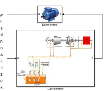
Based on the described parallel flow and flow feedback principles, the final model is made. This final model has to meet the conditions which are described in section 4.4.4. The final model consist of an integration part and an iterative model. Figure 14 shows the integration model, where the Lube oil system block is a subsystem which contains the iterative model. This iterative model is shown in Figure 15 and it can be seen that it contains all the components that were described in chapter 2. In the following paragraphs, the function of each block in the model is explained separately. The centrifugal pumps, electric motors and orifice
plate are already explained in the iterative model and integration model and these are the same in the final model.
Figure 15: Final model, iterative part