Interconverting Models of Gray Matrix and Geographic Coordinates Based on Space Analytic Geometry

Interconverting Models of Gray Matrix and Geographic

Coordinates Based on Space Analytic Geometry

*

Ni Zhan#, Liang Lin, Ling Lou

College of Science, Guilin University of Technology, Guilin, China Email: #_{[email protected]}

Received November 5, 2012; revised December 5, 2012; accepted December 13, 2012

ABSTRACT

With the progress and development of science, the synchronous satellite as the high-tech product is taken something more and more seriously by all countries. Converting gray value matrix into geographic coordinates becomes more and more important. This paper establishes the models for interconverting row and column of gray value matrix which de- tected by the infrared detectors on synchronous satellites and geographic coordinates based on the related theorems and properties of space analytic geometry. We draw satellite cloud image with the data of gray matrix in MATLAB, convert coastline’s latitude and longitude coordinates into row and column coordinates of a gray matrix according via these models when the sub-satellite point’s row and column coordinates and geographic coordinates are given, then add coast-lines to the original satellite cloud image with the transformation data. We find that coast-lines completely match with the bump characteristics of satellite cloud image, and that verify the correctness of the models.

Keywords: Space Analytic Geometry; Satellite Cloud Image; Geographic Coordinates; Gray Value Matrix; Coastline

1. Introduction

Satellite cloud image plays an important role in the sci- entific research of mastering atmospheric circulation, medium-and long-term weather forecast and disastrous weather and so on. It is drawn with grayscale data which converted from the temperature data over the Earth de- tected by infrared detector on geosynchronous satellite. It captures the distribution of clouds in the atmosphere, to find the weather system and verify the correctness of surface weather maps that have been drawn. Sub-satellite point represented by geographic latitude and longitude is the point at which a line between the satellite and the centre of the Earth intersects the Earth’s surface. Infrared detector scans sampling in accordance with stepping an- gle (north-south direction) and row scanning angle. The satellite probe data is a gray value matrix, each element of the matrix corresponds to a sampling point of the Earth or extraterrestrial. Established the models that in- terconvert non-negative elements of grayscale matrix and geographic coordinates, taking up north down south left west right east as the rule, is not only a way to estimate the distance between each probe point, but also a method to the add coast-lines to a satellite cloud image accurately. In meteorological research and service, it is often posi-

tioning and reading the value of geographic coordinates in satellite cloud image, the low resolution and small image make positioning accuracy in a low level. There- fore it produces positioning error, which has an influence on forecast accuracy and research accuracy. Calculating the conversion formulas have attracted much attention, in particular among people interested in the remote sensing technology and meteorology.

Zhang Qingshan [1] uses linear regression to estimate satellite spin axis vector in the nephogram imaging pro- cess, calculating the exact position and attitude of the satellite on the basis of geographic coordinates, trans- forming the nephogram coordinates to geographic coor- dinates. Wang Guanghui & Chen Biao [2] use the me- thod of rotating spherical coordinates system to calculate longitude and latitude of the 2048th sampling point in scanline scanning by High Resolution Infrared Radiation Sounder. Zhang Jinjin & Liang Hongyou [3] design al- gorithms whose objective is to converse plane coordi- nates to latitude and longitude coordinates use of IDL. Dong Minglun & Zhou Jiong [4] educe the relationship between Cartesian conversions and Geographic conver- sions according to visual imaging principle of synchro- nous meteorological satellite. George P. Gerdan & Rod- ney E. Deakin [5] review and analyze six published tech- niques of Cartesian-to-geographic conversion, which are regarded as representative of the numerous published methods, found that Lin & Wang’s method is appreciably

*_{This research was supported by the Guangxi Natural Science}

Founda-tion of China under the Grant No. 2011GXNSFA018149.

faster than the other five methods.

In this paper, we do some research in conversion me- thods which could transform the row and column coor- dinates corresponding to gray value matrix into latitude and longitude coordinates, apply the geometry knowl- edge and ellipsoidal coordinates to establish conversion models, finally verify the models with the measured data consists of gray value matrix and latitude and longitude coordinates of coastline. This method which may be of use to practitioners is simple and feasible. The innovation of this paper is setting parameters for the sub-satellite point’s latitude and longitude coordinates to establish models by using related theorems of space analytic ge- ometry, makes the models more general, suitable for wherever the sub- satellite point located. Since the mo- dels have analytical solution, it improves the accuracy and is a relatively simple method.

The paper is organized as follows. Section 2 is the main part of this paper, converting coordinates models are investigated. Section 3 presents a numerical example to show the applications of the proposed methods. Sec- tion 4 concludes this paper with a brief summary.

2. Converting Coordinates Models

In order to converse row and column coordinates

 

i j,

from geographic coordinates



 ,



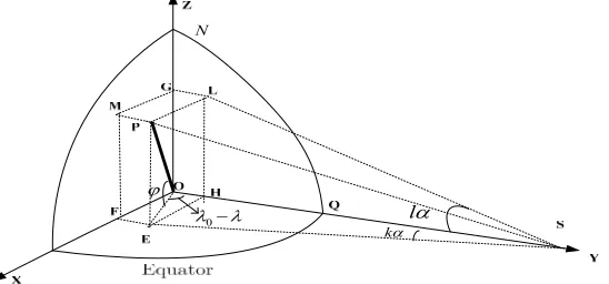
, one important thing is to ensure the corresponding latitude and longitude of each element in gray value matrix. We consider the Earth as an ideal ellipsoid, which obtain through an ellipse ro-tates around the line connecting the north and the south poles. The semi-major of the ellipsoid is equatorial radius, semi-minor axes is polar radius. We take eighth of ellip-soid to create a three-dimensional coordinate system for research.

X, Y, Z 3-D coordinates have an origin at the centre of the ellipsoid as shown in Figure 1. The X-Y plane is the

equatorial plane of the ellipsoid (the origin of latitudes), the Z-axis is in the direction of the rotational axis of the ellipsoid of revolution, the Y-axis is in the direction of

the line connecting the infrared detector on geosynchro- nous satellite and the centre of the ellipsoid, which inter- sects with Earth’s surface at sub-satellite point (Q), and the X-axis is advanced 90˚ west along the equator. The distance between the infrared detector and the centre of the ellipsoid is OS line remarked as c. P is an arbitrary sampling point on the Earth. The point E is referred to as the projection of P in the X-Y plane.Likewise, L is the projection of P in the Y-Z plane and M is the projection of P in the X-Z plane. Drop a perpen- dicular EF from E to X axis, and EH is the perpendicular to Y axis through the point E, PM, PL are the perpen- diculars to X axis and Y axis through the point P, respec- tively.

The sampling point’s row and column coordinates in the gray matrix can be expressed as , 3-D coor-

dinates expressed as

 

,

P i j



, ,



P x y z

,

P

, latitude and longitude coordinates expressed as



 



,  and  repre- sent longitude and latitude of sampling point respectively. Thus sub-satellite point’s row and column coordinates can be expressed as Q I J

 

,



0,0

Q 

, latitude and longitude coordinates expressed as . Referring to Figure 1, the following relationships will be of use in the

deriva-tions that follow.



x OF EH, y OH EF, z OG PE,

POE 

  , HOE 0 , OPr

The stepping angle of infrared detector is. OQ = a

and ON = b are the semi-major and semi-minor axes of the ellipsoid. Let and represent the total number of row scanning and column scanning, respectively, which count from Q to P. Correspondingly, the detector turns respectively

k

k l

and lradians in the direction of horizontal and vertical.

An ellipsoid is a closed quadric surface that is a three dimensional analogue of an ellipse. The standard equa- tion of an ellipsoid centered at the origin of a Cartesian coordinate system is

2 2 2

2 2 2 1

x y z

a a b  (1)

0   

kl

[image:2.595.164.438.586.714.2]

N

The surface of the ellipsoid may be parameterized in several ways. One choice which singles out the “z”-axis is:







0 0 cos sin cos cos sin x r y r z r



               

 (2)

From right-angled triangle EHS we get:

 

tan k x

c y

 

 From right-angled triangle LHS we get:

 

tan k x

c y    Build equations:



  



  

2 2 2 2 tan tan 1

x c y k

z c y l

x z y a a b                       (3)

From Equations (2) and (3) we work out:













0 0 0 cos sin 1_arctan cos cos 1 sin arctan cos cos r k c r r l c r                   _ _             _{  }    (4)

where ₂1 ₂

cos sin r a b      _          .

In this paper, we take sub-satellite point as the initial point to compute the row and column coordinates of the four cardinal directions: north, east, south and west. Therefore, we divide the ellipse into four quadrants tak-ing sub-satellite point as origin , and discuss in four cases to converse (k, l) to (i, j). In the first quadrant, the for-mula can be:

i I k j J l

     

 (5) when i I j , J.

Put (4) into (5), that is:













0 0 0 cos sin 1 arctan cos cos

1_arctan sin cos cos a i I c a a j J c a       

when iI j, J.

Similarly, we can get the other three quadrants’ for- mulas:

The second quadrant:













0 0 0 cos sin 1_arctan cos cos 1 sin arctan cos cos a i I c a a j J c a                    _ _               _{   }    (7)

when i I j , J. The third quadrant:













0 0 0 cos sin 1_arctan cos cos 1 sin arctan cos cos a i I c a a j J c a                    _ _               _{   }    (8)

when i I j , J. The fourth quadrant:













0 0 0 cos sin 1 arctan cos cos

1_arctan sin cos cos a i I c a a j J c a                    _ _                _{ }     (9)

when iI j, J.

The four Formulae (6)-(9) above are the models that converse longitude and latitude coordinates into row and column coordinates.

Conversion from geographic coordinates to row and column coordinates is a simple operation. Inverse com- putations, on the other hand, are a little complex, now we want to use (i, j) to deduct



 ,



. Consider the case of the second quadrant for example: putthe first two equa- tions of (3) into the third equation of (3), we have:





2 2

 

2

 

2

2 2

tan tan

1

k l y

c y

a b a

 

 

2

   

 

   (10)

Let

 

 

2 2

2 2

tan k tan l d

a b

 

  , we get





2 2

2 1

y c y d

a

   , the solutions to this quadratic equa-

tion can be found directly from the quadratic formula.

           _{ }                _{ }       (6)

Solve for y:

2 2 2

2

+1 1

a cd a a d c d y

a d

 



 . As , so

we take

0

y

2 2 2

2

+ +

1



 



  



2 2

0

tan tan

arctan

arctan

x c y k

z c y l

z

x y

x y

 



 

 

 

 



 _



 

    

(11)

Let tan

 

k m,tan

 

l n, from (10) we obtain

2 2 2

2

1 1

a cd a a d c d y

a d

  



 , put it into (11), we get (12) where









tan

m I i  , ntan





J j







d m₂2 n2₂ a b

  .

The other three equations can be obtained by the same method. We do not list all the cases in this paper.

3. A Numerical Example

In this section, we present our experiment results. It may be helpful to illustrate these models in a constructed ex- ample simple enough that an analytical approach is pos- sible. The results reported here are based on 2288 × 2288 gray value matrix detected by a satellite detection which is located at 0˚N latitude and 86.5˚E longitude, that is . Given the distance between sat- ellite and the center of Earth is 42,164,000 m, that is c = 42164000 m. The detection scans by the stepping angle of 140 micro-arcs, that is



0,0





86.5, 0

Q  Q



0.00014

  . Given a = 6378136.5 m, b = 6356751.8 m.

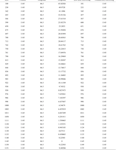
We select arbitrarily 40 sampling points on the column 1145 to test the models. Use (7) to convert the sampling points’ row and column coordinates into longitude and latitude coordinates, then we want to use the results to calculate the row and column coordinates via (6)-(9), results as follow:

From Table 1 it can be seen that after converting the

row and column coordinates into geographical coordi- nates, then converting back, there exists error of 1 - 3 pixels between the row coordinates before and after con- version in nine of the sampling points. The rest coordi- nates are wholly consistent. The error of 1 - 3 pixels is

rounding error which falls within the acceptable range. And results proved that the models are reasonable.

In reference [4], the calculated results exists 0.3 pixel error between the rows and 4.6 pixel between the col- umns, the models of this paper based on previous studies have higher accuracy.

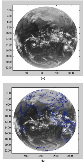
Draw satellite cloud image with the data of gray value matrix in MATLAB [6], as shown in Figure 2(a), add

coast-lines into satellite cloud image, shown in Figure 2(b).

Convert the data of coastline’s longitude and latitude

(a)

(b)

Figure 2. (a) Satellite cloud image; (b) Satellite cloud image with coast-lines.





2 2 2

2

2 2

2 2 2 2 2

2

2 2

2 2

0 _{2 2 2}

1 1 arctan

1 1

1

1 arctan

1

a cd a a d dc n c

a d

c a a d dc a cd a a d dc

m

a d a d

m c a a d dc

a cd a d dc



 

  _{  } 

   



 _ _

 

 _{        }

 _{  }

 _{    }

   



   

  

 _{  }



1

  

[image:4.595.332.508.228.570.2] [image:4.595.67.540.613.736.2]

[image:5.595.60.540.110.731.2]

Table 1. Results of converting coordinates.

Row Column Longitude Longitude Row after converting Column after converting

100 1145 86.5 65.82926 101 1145

230 1145 86.5 49.9728 233 1145

342 1145 86.5 41.1886 345 1145

455 1145 86.5 33.91336 457 1145

566 1145 86.5 27.61518 567 1145

599 1145 86.5 25.85278 600 1145

650 1145 86.5 23.2053 651 1145

675 1145 86.5 21.93694 676 1145

697 1145 86.5 20.83494 697 1145

700 1145 86.5 20.68563 700 1145

713 1145 86.5 20.04117 713 1145

742 1145 86.5 18.61763 742 1145

750 1145 86.5 18.22815 750 1145

761 1145 86.5 17.69476 761 1145

790 1145 86.5 16.29969 790 1145

813 1145 86.5 15.20387 813 1145

829 1145 86.5 14.44661 829 1145

844 1145 86.5 13.74017 844 1145

856 1145 86.5 13.17732 856 1145

895 1145 86.5 11.36085 895 1145

903 1145 86.5 10.99046 903 1145

922 1145 86.5 10.11349 922 1145

930 1145 86.5 9.74532 930 1145

950 1145 86.5 8.827475 950 1145

976 1145 86.5 7.639261 976 1145

986 1145 86.5 7.183597 986 1145

998 1145 86.5 6.637687 998 1145

1000 1145 86.5 6.54679 1000 1145

1002 1145 86.5 6.455919 1002 1145

1011 1145 86.5 6.047289 1011 1145

1050 1145 86.5 4.281411 1050 1145

1111 1145 86.5 1.530465 1111 1145

1120 1145 86.5 1.125251 1120 1145

1124 1145 86.5 0.945185 1124 1145

1130 1145 86.5 0.67511 1130 1145

1135 1145 86.5 0.450065 1135 1145

1140 1145 86.5 0.22503 1140 1145

1145 1145 86.5 0 1145 1145

1150 1145 86.5 −0.22503 1149 1145

into row and column coordinates, then add coast-lines into satellite cloud image. We can discover that coast- lines exactly match with the bump characteristics of sat- ellite cloud image. It illustrates the models are reason- able.

4. Conclusions

This paper has presented the methods with analytical solution of interconverting row and column of gray value matrix and geographical coordinates based on the related theorems and properties of space analytic geometry, fi- nally gives acceptable results of a numerical example to verify the correctness of the models.

This work can also be easily applied in satellite image registration and so on. Our future work involves using these models in cloud motion models developed at satel- lite cloud image and analyzing its feasibility.

REFERENCES

[1] Q. S. Zhang, “Method of Static Meteorological Tatellite

Cloud Image Landmark Navigation,” China Academic Journal Electronic Publishing House, Beijing, 1984, pp. 14-20.

[2] G. H. Wang, B. Chen and W. P. He, “Research of Longi-tude and LatiLongi-tude of AVHRR 2048 Based on Polar Coor-dinate Transformation,” Journal of Qingdao University, Vol. 16, No. 3, 2003, pp. 45-48.

[3] J. J. Zhang, H. Y. Liang, X. F. Chen, X. F. Gu, T. Yu and H. B. Ge, “Transformation from Image Panel Coordinate to Latitude and Longitude Coordinate,” Geospatial In-formation, Vol. 8, No. 1, 2010, pp. 63-66.

[4] M. L. Dong and Q. Zhou, “Transforming Relationship between Cartesian Coordinates and Geographical Coor-dinates and Error Analysis,” Marine Forecasts, Vol. 28, No. 2, 2011, pp. 48-54.

[5] G. P. Gerdan and R. E. Deakin, “Transforming Cartesian Coordinates X, Y, Z to Geographical Coordinates φ, λ, h,” The Australian Surveyor, Vol. 44, No. 1, 1999, pp. 55-63. [6] D. Teng, P. Wang, Y.-G. Che and D. Wang, “Realization