Time Varying Vector Autoregressions: Efficient Estimation, Random Inertia and Random Mean

Munich Personal RePEc Archive

Time-Varying Vector Autoregressions:

Efficient Estimation, Random Inertia and

Random Mean

Legrand, Romain

24 August 2019

Online at

https://mpra.ub.uni-muenchen.de/95707/

Time-Varying Vector Autoregressions: Efficient

Estimation, Random Inertia and Random Mean

Romain Legrand

This version: April 2019

Abstract

Time-varying VAR models represent fundamental tools for the anticipation and analysis of eco-nomic crises. Yet they remain subject to a number of limitations. The conventional random walk assumption used for the dynamic parameters appears excessively restrictive, and the existing es-timation procedures are largely inefficient. This paper improves on the existing methodologies in four directions:

i) it introduces a general time-varying VAR model which relaxes the standard random walk as-sumption and defines the dynamic parameters as general autoregressive processes with equation-specific mean values and autoregressive coefficients.

ii) it develops an efficient estimation algorithm for the model which proceeds equation by equa-tion and combines the tradiequa-tional Kalman filter approach with the recent precision sampler methodology.

iii) it develops extensions to estimate endogenously the mean values and autoregressive coeffi-cients associated with each dynamic process.

iv) through a case study of the Great Recession in four major economies (Canada, the Euro Area, Japan and the United States), it establishes that forecast accuracy can be significantly improved by using the proposed general time-varying model and its extensions in place of the traditional random walk specification.

JEL Classification: C11, C15, C22, E32, F47.

Keywords: Time-varying coefficients; Stochastic volatility; Bayesian methods; Markov Chain Monte Carlo methods; Forecasting; Great Recession.

1

Introduction

Vector autoregressive models have become the cornerstone of applied macroeconomics. Since the seminal work of Sims (1980), they have been used extensively by financial and economic institutions to perform routine policy analysis and forecasts. While convenient, VAR models with static coefficients and volatility often turn out to be excessively restrictive in capturing the dynamics of time-series, which typically exhibit some form of non-linearity in their behaviours. This motivated the introduction of time-varying coefficients (Canova (1993), Stock and Watson (1996), Cogley (2001), Ciccarelli and Rebucci (2003)) and stochastic volatility (Harvey et al. (1994), Jacquier et al. (1995), Uhlig (1997), Chib et al. (2006)), to account for potential shifts in the transmission mechanism and variance of the underlying disturbances. More recently, the two features have been combined (Cogley and Sargent (2005), Primiceri (2005)) to produce a class of fully time-varying VAR models.

With the events of the Great Recession, time-varying VARs have attracted renewed attention. Part of the literature has focused on the heteroskedasticity of the exogenous shocks (Stock and Watson (2012), Doh and Connolly (2013), Bijsterbosch and Falagiarda (2014), Gambetti and Musso (2017)), primarily interpreting the Great Recession as an episode of sharp volatility of the disturbances affecting the economy. Rather, other works have emphasized the changes in the transmission mechanism (Baumeister and Benati (2010), Benati and Lubik (2014), Ellington et al. (2017)), and view the Great Recession as a period of altered response of macroeconomic variables to economic policy. In either case, there is strong evidence that accounting for time variation is crucial to the accuracy of policy analysis and forecasts in a context of crisis. Conse-quently, time-varying VARs should represent a benchmark tool to predict economic downturns and their evolutions.

However, these models remain subject to limitations of both theoretical and methodological order. On the theoretical side, the literature has widely adopted the random walk specification for the laws of motion of the different dynamic parameters. Denoting for instance byθtany one of the dynamic parameters of the VAR model and byǫtthe shock on the process, a random walk law of motion expresses as:

θt=θt−1+ǫt or, equivalently θt= ∞ X

j=0

ǫt−j (1)

A number of attempts have been made to restrict the undesirable properties of the random walk (Ciccarelli and Rebucci (2002), Koop and Korobilis (2010), Nakajima and West (2015), Eisenstat et al. (2016)). These approaches typically address the first issue, but not the second one. They also involve the estimation of a large number of additional parameters, which may generate parsimony issues and substantially complicate the estimation procedure. For these reasons, it is preferable to simply replace (1) by a stationary formulation of the kind:

θt= (1−γ)¯θ+γθt−1+ǫt or, equivalently θt= ¯θ+ ∞ X

j=0

γjǫt−j (2)

with 0 ≤ γ ≤ 1 and ¯θ respectively denoting the autoregressive coefficient and mean terms of the process. Formulation (2) addresses both issues related to the random walk, while remaining conceptually simple. A final issue related with the random walk specification is the homogeneity assumption it sets de facto, as it implies that all the dynamic parameters follow a similar unit-root process. There is yet no legitimate reason to assume that the dynamic parameters of different variables evolve homogeneously. In fact, it is quite likely that different economic variables are characterised by different behaviours of their dynamic coefficients and residual volatilities. For this reason, an equation-by-equation approach seems preferable for the dynamic processes. This leads to reformulate (2) as:

θi,t= (1−γi)¯θi+γiθi,t−1+ǫi,t or, equivalently θi,t = ¯θi+ ∞ X

j=0

γ_ijǫi,t−j i= 1, . . . , n (3)

whereθi,t represents the component ofθt for equationiof the model, andγi and ¯θi respectively denote the equation-specific autoregressive coefficient and mean terms. This specification is suf-ficiently flexible to capture the essential specificities of the behaviours of the different variables included in the model. It creates however new challenges as it becomes crucial to determine the values ofγiand ¯θi properly. This question has attracted considerable attention in the univariate ARCH literature (Jacquier et al. (1994), Kim et al. (1998), Chib et al. (2002), Jacquier et al. (2004)), while contributions on the multivariate side have been more limited. Ciccarelli and Re-bucci (2003), Prado and West (2010) and Lubik and Matthes (2015) propose a general stationary formulation for the law of motion of their time-varying VAR models, but retain the random walk for estimation. Clark and Ravazzolo (2015) test for a stationary stochastic volatility specification with inconclusive results compared to the random walk. Another option consists in estimating the parameters endogenously. Yet limited work has been done in this direction. In a first attempt to determine the mean of the structural shock volatility, Uhlig (1997) relies on a set of Beta prior distributions. Primiceri (2005) questions the random walk assumption and tests for exogenous estimation of the autoregressive coefficients on the dynamic processes. He concludes that no relevant differences exist compared to the homogeneous random walk specification. Mumtaz and Zanetti (2013) endogenously estimate the autoregressive coefficients on stochastic volatility, and obtain coefficients close to the random walk.

formulation proposed by Primiceri (2005) and amended by Del Negro and Primiceri (2015). This approach builds on the algorithm developed by Carter and Kohn (1994), which uses a two-pass procedure based on the Kalman filter. The procedure is rather sophisticated and unintuitive. Also, the multiple loops through time and the building of the states in a recursive fashion may considerably slow down the estimation. This is especially true for large models for which the Primiceri (2005) approach becomes very inefficient. Yet the recent literature has emphasized the importance of large information sets (Banbura et al. (2010), Carriero et al. (2015), Gian-none et al. (2015), Kalli and Griffin (2018)), establishing that large systems perform better than smaller systems in forecasting and structural analysis.

Different strategies have been adopted to overcome this inefficiency issue. Carriero et al. (2016) propose to estimate their large Bayesian VAR model equation by equation rather than jointly. Doing so considerably reduces the computational complexity of the estimation algorithm, render-ing the estimation of large VARs feasible. Nevertheless, their model is only partially time-varyrender-ing as it involves stochastic volatility but leaves the residual covariance and VAR coefficient parts of the model static. Hence, it is not yet established how much efficiency gains can be obtained from their methodology once applied to a fully time-varying model of the kind of Primiceri (2005). An alternative strategy has been proposed by Chan and Eisenstat (2018). The authors develop a precision sampler which replaces the traditional Carter and Kohn (1994) algorithm with a full sample formulation relying on sparse matrices. Significant efficiency gains are reported (of the order of 15-30%). Nevertheless, the few papers using the methodology so far (Chan and Jeliazkov (2009), Chan (2013)) have been limited to small dimensional parameters, and it is yet uncertain how well the precision sampler performs in larger dimensions. As the two approaches are not mutually exclusive, a natural strategy suggests to combine them in the hope of optimising the efficiency of the estimation procedure.

Based on these considerations, this paper contributes to the literature in four directions. First, it introduces a general, fully time-varying VAR model which is formulated on an equation by equa-tion basis. For each dynamic parameter, the random walk assumpequa-tion is relaxed and replaced with a general autoregressive process with equation-specific mean values and autoregressive co-efficients. Second, it proposes an optimal sampling algorithm for the model which combines the equation by equation estimation procedure of Carriero et al. (2016) with the precision sampler of Chan and Eisenstat (2018) and the traditional Carter and Kohn (1994) methodology1. It shows that the procedure provides considerable efficiency gains, even on large models. Third, it proposes extensions to endogenously estimate the mean terms and autoregressive coefficients associated with the laws of motion of each dynamic parameter. The employed priors are infor-mative and aim at getting closer to the underlying data generating process. Finally, the paper conducts a case study on the Great Recession. The exercise is realised on a large time-varying VAR comprising 12 variables, estimated for four major economies (Canada, the European Union, Japan and the United States). It establishes that the random walk is unambiguously rejected as a suitable formulation for forecasting purposes, and further shows that the extensions

outper-1

form the base stationary formulation in terms of forecast accuracy. Following, it suggests that the crisis could have been better predicted with a proper use of time-varying VAR models.

The remaining of the paper is organised as follows: section 2 introduces the general time-varying model and provides the details of the estimation procedures; section 3 discusses the efficiency of different competing methodologies and introduce the optimal sampling algorithm; section 4 develops the extensions allowing for endogenous estimation of the autoregressive coefficients (random inertia) and mean terms (random mean) of the dynamic parameters; section 5 presents the results of the case study on the Great Recession and discusses the benefits of the general time-varying model and its extensions in terms of forecast accuracy; section 6 concludes.

2

A general time-varying model

2.1 The model

Consider the general time-varying model:

yt=Ctzt+A1,tyt−1+· · ·+Ap,tyt−p+εt t= 1,· · ·, T , εt∼ N(0,Σt) (4)

ytis a n×1 vector of observed endogenous variables, zt is am×1 vector of observed exogenous variables such as constant or trends, andεtis an×1 vector of reduced-form residuals. The resid-uals are heteroskedastic disturbances following a normal distribution with variance-covariance matrixΣt. Ct, A1,t,· · ·, Ap,t are matrices of time-varying VAR coefficients comfortable with zt and the lagged values ofyt. Stacking in a vectorβt the set of VAR coefficients, (4) rewrites:

yt=Xtβt+εt (5)

with:

Xt=In⊗xt , xt= zt′ y′t−1 · · · yt′−p

, βt=vec(Bt) , Bt= Ct A1,t · · · Ap,t′ (6)

Considering specifically rowiof (5), the equation for variablei of the model rewrites:

yi,t =xtβi,t+εi,t (7)

where βi,t is the k×1 vector obtained from column i of Bt. Stacking (7) over the T sample periods yields a full sample formulation for equationi:

yi =Xβi+εi (8)

with:

yi = 

   

yi,1 yi,2

.. . yi,T     

, X =      

x1 0 · · · 0

0 x2 . .. ...

..

. . .. ... 0 0 · · · 0 xT

     

, βi = 

   

βi,1 βi,2

.. . βi,T     

, εi = 

   

εi,1 εi,2

.. . εi,T      (9)

The variance-covariance matrixΣt for the reduced form residuals is decomposed into:

∆t (and ∆−_t1) are unit lower triangular matrix, while Λt is a diagonal matrix with positive diagonal entries, taking the form:

∆t=      

1 0 · · · 0

δ21,t 1 . .. ... ..

. . .. . .. 0

δn1,t · · · δn(n−1),t 1      

, Λt=      

s1 exp(λ1,t) 0 · · · 0

0 s2 exp(λ2,t) . .. ...

..

. . .. . .. 0

0 · · · 0 sn exp(λn,t)       (11)

The triangular decomposition of the variance-covariance matrixΣtimplemented in (10) is com-mon in time-series models.2 Λt represents the volatility components of Σt, each si being a positive scaling term which represents the equilibrium value of the residual variance of equation

i of the model. On the other hand, ∆t can be interpreted as the (inverse) covariance compo-nent of Σt. Denoting by δi,t the vector of non-zero and non-one terms in row i of ∆t so that

δi,t = (δi1,t · · · δi(i−1),t)′,δi,t then represents the covariance between the residual of equation

iof the model and the other shocks.

The dynamics of the model time-varying parameters is specified as follows:

βi,t = (1−ρi)bi+ρiβi,t−1+ξi,t t= 2,3, . . . , T ξi,t ∼ N(0,Ωi)

βi,1 =bi+ξi,1 t= 1 ξi,1 ∼ N (0, τΩi) λi,t=γiλi,t−1+νi,t t= 2,3, . . . , T νi,t ∼ N(0, φi)

λi,1 =νi,1 t= 1 νi,1∼ N (0, µφi)

δi,t = (1−αi)di+αiδi,t−1+ηi,t t= 2,3, . . . , T ηi,t ∼ N(0,Ψi)

δi,1 =di+ηi,1 t= 1 ηi,1 ∼ N(0, ǫΨi) (12)

ρi, γi and αi represent equation-specific autoregressive coefficients while bi,si and di represent the equation-specific mean values of the processes. These are treated for now as exogenously set hyperparameters, but the assumption will be relaxed in section 4. Clearly, each law of motion nests the usual random walk as a special case setting the autoregressive coefficient to 1. For each process, the initial period is formulated consistently with the overall dynamics of the parameters. The mean corresponds to the unconditional expectation of the process, while the variance is scaled by the hyperparametersτ, µ, ǫ >1 to account for the greater uncertainty associated with the initial period. All the innovations in the model are assumed to be jointly normally distributed with the following assumptions on the variance covariance matrix:

V ar     εt ξi,t νi,t ηi,t     =    

Σt 0 0 0

0 Ωi 0 0

0 0 φi 0

0 0 0 Ψi



  

(13)

This concludes the description of the model. Fori= 1, . . . , n, the parameters of interest to be estimated are: the dynamic VAR coefficients βi ; the dynamic volatility terms λi; the dynamic covariance terms δi; and the associated variance-covariance parametersΩi,φi and Ψi. To these six base parameters must be added the parameterri,t whose role will be clarified shortly.

2

2.2 Bayes rule

Following most of the literature, Bayesian methods are used to evaluate the posterior distribu-tions of the parameters of interest. Given the model, Bayes rule is given by:

π(β,Ω, λ, φ, δ,Ψ, r|y)∝f(y|β, λ, δ, r)

×

n Y

i=1

π(βi|Ωi)π(Ωi) ! _n

Y

i=1

π(λi|φi)π(φi) ! _n

Y

i=2

π(δi|Ψi)π(Ψi) ! _n

Y

i=1

T Y

t=1 π(ri,t)

!

(14)

2.3 Likelihood function

Starting from (5) and rearranging, a first formulation of the likelihood function obtains as:

f(y|β, λ, δ, r) = (2π)−nT /2 n Y

i=1 s−_i T /2

!

× exp −1

2 n X

i=1

n

λ′_i1T + (yi−Xβi+Eiδi)′ s−i 1Λi˜ (yi−Xβi+Eiδi) o

!

(15)

with:

λi= 

   

λi,1 λi,2

.. . λi,T     

1T =      1 1 .. . 1      ˜

Λi =diag(˜λi) ˜λi = 

   

exp(−λi,1) exp(−λi,2)

.. .

exp(−λi,T) 

   

Ei =       ε′

−i,1 0 · · · 0

0 ε′_−i,2 . .. ... ..

. . .. ... 0

0 · · · 0 ε′_−i,T

     

ε−i,t = 

   

ε1,t

ε2,t .. .

εi−1,t 

   

δi = 

   

δi,1 δi,2

.. . δi,T      (16)

(15) proves convenient for the estimation of βi and δi, but does not provide any conjugacy for λi due to the presence of the exponential term ˜Λi. This is a well-known issue of models with stochastic volatility and the most efficient solution is the so-called normal offset mixture representation proposed by Kim et al. (1998). The procedure consists in reformulating the likelihood function in terms of the transformed shocket= (∆−t1Λ

1/2

t )−1εt. It is trivially shown thatet is a vector of structural shock withet∼ N(0, In). Considering specifically the shockei,t in the vector, squaring, taking logs and rearranging eventually yields:

ˆ

ei,t= log(e2i,t) = ˆyi,t−λi,t yˆi,t = log(si−1(εi,t+δ′i,tε−i,t)2) (17)

ˆ

ei,t follows a log chi-squared distribution which does not grant any conjugacy. Kim et al. (1998) thus propose to approximate the shock as an offset mixture of normal distributions. The ap-proximation is given by:

ˆ

ei,t≈

7

X

j=1

The values for mj, vj and qj can be found in Table 4 of Kim et al. (1998). The constants mj and vj respectively represent the mean and variance components of the normally distributed random variablezj. ri,t is a categorical random variable taking discrete valuesj = 1, . . . ,7,the probability of obtaining each value being equal toqj. Finally,✶(ri,t=j) is an indicator function taking a value of 1 if ri,t = j, and a value of 0 otherwise. To draw from the log chi-squared distribution, the mixture first randomly draws a value for ri,t from its categorical distribution; onceri,t is known, its value determines which component zj of the mixture is selected. eˆi,t then turns into a regular normal random variable with meanmj and variancevj. Given (17) and the offset mixture (18), an approximation of the likelihood function obtains as:

f(y|β, λ, δ, r) = n Y i=1 T Y t=1 7 X j=1

✶(ri,t=j)

(2πvj)−1/2exp

−1

2

(ˆyi,t−λi,t−mj)2

vj

(19)

For the estimation of λi, a more convenient joint formulation can be adopted. Defining ri = (ri,1 . . . ri,T)′, denoting by J any possible value for ri, by mJ and vJ the resulting mean and variance vectors, and defining VJ = diag(vJ), the likelihood function rewrites as a mixture of multivariate normal distributions:

f(y|β, λ, δ, r)

= n Y i=1 J X

✶(ri =J)

(2π)−T /2|VJ|−1/2exp

−1

2(ˆyi−λi−mJ) ′_V−1

J (ˆyi−λi−mJ)

(20)

with:

ˆ

yi = ˆyi,1 yˆi,2 . . . yˆi,T′ =log(s−_i 1Qi) Qi = (εi+Eiδi)2 (21)

2.4 Priors

The priors for the dynamic parametersβi,λi and δi follow the precision sampler formulation of Chan and Eisenstat (2018).3 Consider first the VAR coefficientsβi. Starting from (12), the law of motion can be expressed in compact form as:

     

Ik 0 · · · 0

−ρiIk Ik . .. ... ..

. . .. . .. 0

0 · · · −ρiIk Ik           

βi,1 βi,2

.. . βi,T      =      bi (1−ρi)bi

.. . (1−ρi)bi

     +     

ξi,1 ξi,2

.. . ξi,T      (22) or:

(Fi⊗Ik) βi = ¯bi+ξi Fi=      

1 0 · · · 0

−ρi 1 . .. ... ..

. . .. ... 0 0 · · · −ρi 1

      ¯

bi =      bi (1−ρi)bi

.. . (1−ρi)bi



   

ξi = 

   

ξi,1 ξi,2

.. . ξi,T      (23) 3

Also:

V ar(ξi) =      

τΩi 0 · · · 0

0 Ωi . .. ... ..

. . .. ... 0 0 · · · 0 Ωi

     

=Iτ⊗Ωi Iτ =      

τ 0 · · · 0

0 1 . .. ... ..

. . .. ... 0 0 · · · 0 1

      (24)

(23) and (24) respectively implyβi = (Fi⊗Ik)−1¯bi+ (Fi⊗Ik)−1ξi andξi∼ N(0, Iτ⊗Ωi). From this and rearranging, the prior distribution eventually obtains as:

π(βi|Ωi)∼ N (βi0 ,Ωi0) βi0 = 1T ⊗bi Ωi0 = (Fi′ Iτ−1 Fi⊗Ω−i 1)−1 (25)

Using forλi and δi equivalent procedures and notations, it is straightforward to obtain:

π(λi|φi)∼ N (0,Φi0) Φi0 =φi(G′iIµ−1Gi)−1

π(δi|Ψi)∼ N(δi0 ,Ψi0) δi0 = 1T ⊗di Ψi0= (Hi′ Iǫ−1 Hi⊗Ψ−i 1)−1 (26)

For the priors of the variance-covariance parametersΩi, φi andΨi, the choice is that of standard inverse Wishart and inverse Gamma distributions. Precisely:

π(Ωi)∼IW (ζ0,Υ0) π(φi)∼IG

κ 0 2 , ω0 2

π(Ψi) ∼IW (ϕ0,Θ0) (27)

Finally, from (18), it is immediate that the prior distribution forri,t is categorical:

π(ri,t)∼Cat(q1, . . . , q7) (28)

2.5 Posteriors for the dynamic parameters

The joint posterior obtained from (14) is analytically intractable. Following standard practices, the marginal posteriors are estimated from a Gibbs sampling algorithm relying on conditional distributions. The conditional posteriors of the dynamic parameters are first derived in the con-text of the precision sampler of Chan and Eisenstat (2018).

Forβi, Bayes rule (14) implies π(βi|y,\βi) ∝f(y|β, λ, δ, r)π(βi|Ωi).4 From the likelihood (15), the prior (25) and rearranging, it follows that:

π(βi|y,\βi)∼ N( ¯βi,Ωi)¯ with: ¯

Ωi = (s−_i1X′Λi˜ X+F_i′ I_τ−1 Fi⊗Ω−_i 1)−1 ¯

βi = ¯Ωi(s−i 1X′Λi[˜ yi+Eiδi] +Fi′Iτ−1Fi1T ⊗Ω−i 1bi) (29)

For λi, Bayes rule (14) implies π(λi|y,\λi) ∝ f(y|β, λ, δ, r)π(λi|φi). From the approximate likelihood (20), the prior (26) and rearranging, it follows that:

π(λi|y,\λi) ∼ N(¯λi,Φi)¯ with: ¯

Φi = (V_J−1+φ_i−1G′_iI_µ−1Gi)−1 λ¯i= ¯Φi(V_J−1[ˆyi−mJ]) (30)

4

Forθiany parameter,π(θi|\θi) is used to denote the density ofθiconditional on all the model parameters except

For δi, Bayes rule (14) implies π(δi|y,\δi) ∝ f(y|β, λ, δ, r)π(δi|Ψi). From the likelihood (15), the prior (26) and rearranging, it follows that:

π(δi|y,\δi)∼ N(¯δi,Ψi)¯ with: ¯

Ψi= (s−_i1E′_iΛi˜ Ei+Hi′ I−ǫ Hi⊗Ψ−i 1)−1 ¯δi = ¯Ψi(−s−i 1E′iΛi˜ εi+Hi′I−ǫHi1T ⊗Ψ−i 1di) (31)

For incoming developments, it is worth mentioning that as an alternative to the precision sampler, the conditional posteriors for the dynamic parameters can be derived from the algorithm of Carter and Kohn (1994). The algorithm is standard and the details are deferred to Appendix A in order to save space.

2.6 Posteriors for the other parameters

For Ωi, Bayes rule (14) implies π(Ωi|y,\Ωi) ∝ π(βi|Ωi)π(Ωi). From the priors (25) and (27) then rearranging, it follows that:

π(Ωi|y,\Ωi)∼IW(¯ζ,Υi)¯ with: ζ¯=T +ζ0 Υi¯ = ˜Bi+ Υ0

˜

Bi = (Bi−1′T ⊗bi) (Fi′ Iτ−1 Fi)(Bi−1′T ⊗bi)′ Bi= (βi,1 βi,2 · · · βi,T) (32)

Forφi, Bayes rule (14) impliesπ(φi|y,\φi)∝π(λi|φi)π(φi). From the priors (26) and (27) then rearranging, it follows that:

π(φi|y,\φi)∼IG(¯κ,ω¯i) with: κ¯=

T +κ0

2 ω¯i =

λ_i′(G′_iIµ−1Gi)λi+ω0

2 (33)

For Ψi, Bayes rule (14) implies π(Ψi|y,\Ψi) ∝ π(δi|Ψi)π(Ψi). From the priors (26) and (27) then rearranging, it follows that:

π(Ψi|y,\Ψi)∼IW( ¯ϕ,Θi)¯ with: ϕ¯=T +ϕ0 Θi¯ = ˜Di+ Θ0

˜

Di= (Di−1′T ⊗di)(Hi′ I−ǫ Hi)(Di−1′T ⊗di)′ Di = (δi,1 δi,2 · · · δi,T) (34)

Finally, forri,t, Bayes rule (14) impliesπ(ri,t|y,\ri,t)∝f(y|β, λ, δ, r)π(ri,t). From the approxi-mate likelihood (19) and the prior (28), it follows immediately that:

π(ri,t|y,\ri,t)∼Cat(¯q1, . . . ,q¯7) with: q¯j = (2πvj)−1/2exp

−1

2

(ˆyi,t−λi,t−mj)2

vj

qj (35)

2.7 MCMC algorithm

A preliminary, naive version of the MCMC algorithm for the general time-varying model is now introduced. This version fully relies on the precision sampler procedure, and its performance is discussed in the incoming section. The algorithm consists in a 7-step procedure, as follows:

Algorithm 1: MCMC algorithm for the general time-varying model:

1. Fori= 1, . . . , n, sampleλi equation by equation from: π(λi|y,\λi)∼ N(¯λi,Φi).¯

2. Fori= 1, . . . , n, sampleβi equation by equation from: π(βi|y,\βi)∼ N( ¯βi,Ωi¯ ).

4. Fori= 1, . . . , n, sampleΩi equation by equation from: π(Ωi|y,\Ωi)∼IW(¯ζ,Υi).¯

5. Fori= 1, . . . , n, sampleφi equation by equation from: π(φi|y,\φi) ∼IG(¯κ,ω¯i).

6. Fori= 2, . . . , n, sampleΨi equation by equation from: π(Ψi|y,\Ψi) ∼IW( ¯ϕ,Θi).¯

7. Fori= 1, . . . , nand t= 1, . . . , T, sample ri,t from: π(ri,t|y,\ri,t) ∼Cat(¯q1, . . . ,q¯7).

Observe that the ordering of the steps in the algorithm differs from the one used for the presen-tation of the model. It introducesλi first, then the other model parameters, and eventually the offset mixture parameters ri,t. This specific ordering is necessary to recover the correct poste-rior distribution whenever the normal offset mixture is used to provide an approximation of the likelihood function. See Del Negro and Primiceri (2015) for details.

3

Efficiency

3.1 Preliminary comparison

As a preliminary exercise, this section discusses the computational efficiency of the MCMC al-gorithm developed in the previous section for the general time-varying model against a number of competing methodologies and different scales of models. The exercise is based on a quarterly macroeconomic model for the US economy, the details of which are introduced in section 55. Three versions of the model are considered. The first is a “small” version of the model which corresponds to the small US economy model of Primiceri (2005) and includes three variables, two lags and a constant. The second “medium” model comprises six variables and three lags. The final “large” model expands the setting to twelve variables and four lags6. The three models are estimated on a quarterly sample of sizeT = 160.

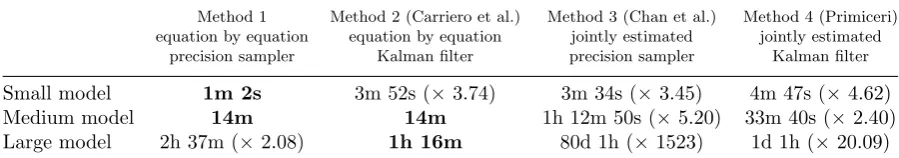
The exercise compares four competing estimation methodologies. The benchmark methodology, labelled as method 1, consists in the general time-varying model introduced in the previous sec-tion, and estimated with Algorithm 1. Again, this procedure combines the equation by equation approach of Carriero et al. (2016) with the precision sampler of Chan and Eisenstat (2018). Following, a natural candidate for comparison consists in a similar model, but estimated jointly rather than equation by equation, and relying on the standard Kalman filter approach rather than on the precision sampler. This corresponds to the standard Primiceri (2005) approach, labelled as method 4. Two other in-between methodologies are considered for the sake of highlighting the respective contributions of the precision sampler and equation by equation approaches. Similarly to Carriero et al. (2016), method 2 adopts an equation by equation procedure but relies on the Kalman filter approach rather than on the precision sampler. At the opposite, in line with Chan and Eisenstat (2018), method 3 uses the precision sampler but estimates the model jointly rather

5

The reader is thus referred to section 5 for a complete presentation of the model, its calibration and a description of the set of variables included along with their transformations.

6

than equation by equation. The results for 10000 repetitions of the algorithm are reported in Table 17.

Method 1 equation by equation

precision sampler

Method 2 (Carriero et al.) equation by equation

Kalman filter

Method 3 (Chan et al.) jointly estimated precision sampler

Method 4 (Primiceri) jointly estimated

Kalman filter

Small model 1m 2s 3m 52s (×3.74) 3m 34s (×3.45) 4m 47s (×4.62) Medium model 14m 14m 1h 12m 50s (×5.20) 33m 40s (×2.40) Large model 2h 37m (×2.08) 1h 16m 80d 1h (×1523) 1d 1h (×20.09)

Bold entry: best methodology; multipliers between brackets are computed respective to the best methodology. Model variables: Small: UR, HICP, STR; Medium: UR, HICP, STR, GDP, LTR, REER; Large: all variables

Table 1: Estimation performances for the different methodologies (for 10000 iterations)

Two main conclusions derive from Table 1. First, estimation of the model equation by equation does improve significantly the computational performance. The gains are variable across esti-mation methodologies and model dimensions, but are always sizable. Smaller dimensions seem to produce the smallest computational benefits, with a bit more than 20% gain in the case of the small model (comparing methods 4 and 2) and around 70% gain in the case of the precision sampler (comparing methods 3 and 1). This is because small models maintain the dimensions of the dynamic parameters low anyway, even when they are estimated jointly. As a consequence, the dimensional issues traditionally arising with the selected algorithms are not too marked and the benefits remain moderate. At high dimensions however, the conclusions are quite different. For the large model the gains become very large, reaching 95% when comparing methods 2 and 4 and exceeding 99.8% when comparing methods 1 and 3. This confirms the lower relative com-putational efficiency of the estimation algorithms at high dimensions, and hence the relevance of the Carriero et al. (2016) approach to reduce the dimensionality of the dynamic parameters in the estimation process.

The second conclusion is that, perhaps surprisingly, the precision sampler of Chan and Eisenstat (2018) does not necessarily improve the computational efficiency of the procedure. Its efficiency seems to be in fact highly related to the dimension of the model. At small dimensions the precision sampler is fully efficient. In the case of the small model, it always represents the best option and is associated with considerable computational gains (almost 75% comparing methods 1 and 2, still more than 25% comparing methods 3 and 4). At medium dimensions the precision sampler plays at par with the Kalman filter when using the equation by equation approach (methods 1 and 2), but is already dominated with a joint estimation approach. At the highest dimension, the precision sampler becomes strictly dominated by the Kalman filter approach, and in the case of a joint estimation (methods 3 and 4) completely breaks down: a simple run of 10000 iterations with the Chan and Eisenstat (2018) methodology would take more than 80 days, rendering the estimation practically infeasible.

7

3.2 Optimal sampling algorithm

Following the conclusions of the previous section it is worth investigating further the properties of the precision sampler, which requires some understanding of the computational details. As discussed in Chan (2013), obtaining a draw from the precision sampler essentially consists in estimating the Cholesky factor of a sparse and banded precision matrix, and then run a back-ward/forward substitution with this Cholesky factor. What Chan (2013) fails to notice is that for a bandwidth ofhin the precision matrix, the number of operations involved for the Cholesky factorisation and the backward/forward substitutions is of the order ofO(h2T) (Boyd and Van-denberghe (2004), p510). Whenhis very small, the computational cost is essentially determined by the sample size T. But as h increases, the flop count becomes quickly dominated by the bandwidthh, and the number of computations can escalate at a very fast rate8. For the general time-varying VAR model developed in section 2, the bandwidth of the matrices involved in the precision sampler methodology corresponds to the dimension of the dynamic parameters at each sample period. This is equal tok for the VAR coefficientsβi, and to a maximum ofn−1 for the residual covariances δi. Because these values can be large, the precision sampler may become inefficient.

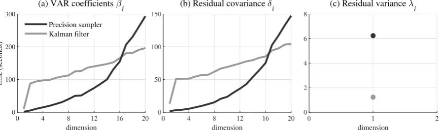
To make this point formal, the respective performances of the precision sampler and the Kalman filter are tested for different dimensions of the parameters βi and δi. λi being always scalar-valued, the comparison is only realised for dimension one. The results are reported in Figure 1:

0 4 8 12 16 20

dimension

0 100 200 300

time (seconds)

(a) VAR coefficients _i

Precision sampler Kalman filter

0 4 8 12 16 20

dimension

0 50 100 150

(b) Residual covariance _i

0 1 2

dimension

0 2 4 6 8

(c) Residual variance _i

Figure 1: Approximate estimation time (in seconds) for 10000 repetitions of the MCMC algorithm at different dimensions

The characteristic quadratic shapes of the precision sampler curves in panels (a) and (b) confirm that the computational cost of the precision sampler grows at some quadratic rate. By contrast, the computational cost of the Kalman filter methodology looks more linear. At small dimen-sions, the comparison is clearly in favor of the precision sampler. At dimension 2 for instance, the precision sampler proves more than 15 times faster than the Kalman filter. The difference gets smaller as the dimension increases, the quadratic inefficiency of the precision sampler eventually outweighing the linear cost of the Kalman filter. A very important result is that the breaking

8

Chan (2013) considers a pure stochastic volatility model whereh= 1. In this case, the computational cost of the precision sampler becomes purely linear in T _{and involves only O(}T_{) operations, as correctly reported by}

point occurs for bothβi and δi at dimension 16. At any dimension smaller than or equal to this value, the precision sampler remains more efficient than the Kalman filter though the gains may vary considerably. At any value above 16 the Kalman filter becomes strictly more efficient, and the precision sampler gets inefficient at a fast rate.

Panel (c) looks surprising. Even though λi is of dimension 1, the most efficient procedure to sample it happens to be the Kalman filter and not the precision sampler. The difference is neat, the Kalman filter procedure being more than five times faster than its precision sampler coun-terpart. There are two explanations for this puzzling result. First, panels (a) and (b) clearly show that dimension 1 constitutes a special case for which the difference between the Kalman filter and the precision sampler is considerably less than for other small dimensions. Second,λi represents a special case in the sense than its state-space formulation in the Kalman filter (see Appendix A, Table 6) is considerably simpler than that ofβi and δi. As the complexity of the formulation represents the main source of inefficiency in the Kalman filter procedure, simplifying the formulation results in considerable efficiency gains. Some gains also apply to the precision sampler, but they are much less given that the underlying state-space formulation is already efficiently vectorised in the procedure.

Based on these considerations, it is possible to propose the following optimal sampling algorithm:

Algorithm 2: Optimal sampling algorithm for the general time-varying model:

1. Fori= 1, . . . , n, sampleλi equation by equation, using the Kalman filter procedure.

2. Fori= 1, . . . , n, sampleβi equation by equation:

If k≤16, use the precision sampler and sample from π(βi|y,\βi)∼ N( ¯βi,Ωi).¯ If k >16, use the Kalman filter procedure.

3. Fori= 2, . . . , n, sampleδi equation by equation:

If n−1≤16, use only the precision sampler and sample fromπ(δi|y,\δi)∼ N(¯δi,Ψi).¯ If n−1>16, use first the precision sampler fori= 1,· · ·,17 and sample from

π(δi|y,\δi)∼ N(¯δi,Ψ¯i); then use the Kalman filter fori= 18,· · ·, n.

4. Fori= 1, . . . , n, sampleΩi equation by equation from: π(Ωi|y,\Ωi)∼IW(¯ζ,Υi).¯

5. Fori= 1, . . . , n, sampleφi equation by equation from: π(φi|y,\φi) ∼IG(¯κ,ω¯i).

6. Fori= 2, . . . , n, sampleΨi equation by equation from: π(Ψi|y,\Ψi) ∼IW( ¯ϕ,Θi).¯

7. Fori= 1, . . . , nand t= 1, . . . , T, sample ri,t from: π(ri,t|y,\ri,t) ∼Cat(¯q1, . . . ,q¯7).

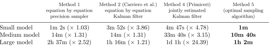
Method 1 equation by equation

precision sampler

Method 2 (Carriero et al.) equation by equation

Kalman filter

Method 4 (Primiceri) jointly estimated

Kalman filter

Method 5 (optimal sampling

algorithm)

Small model 1m 2s (×1.03) 3m 52s (×3.86) 4m 47s (×4.78) 1m Medium model 14m (×1.31) 14m (×1.31) 33m 40s (×3.15) 10m 40s Large model 2h 37m (×2.52) 1h 16m (×1.21) 1d 1h (×24.39) 1h 2m

Bold entry: best methodology; multipliers between brackets are computed respective to the best methodology. Model variables: Small: UR, HICP, STR; Medium: UR, HICP, STR, GDP, LTR, REER; Large: all variables

Table 2: Estimation performances for the different methodologies (for 10000 iterations)

As expected, the optimal sampling algorithm represents the most efficient methodology in all cases. The gains are minimal at the smallest dimension and hardly reach 3% compared to method 1. This is because the two methodologies are very similar, the only difference residing in the fact that method 5 replaces the precision sampler by the Kalman filter to sampleλi. The gains become more sizable for the medium and large model where they respectively exceed 30% and 20% compared to the best alternative. In the case of a large model with many iterations, the benefit of the optimal sampling algorithm becomes considerable, even compared to the efficient equation by equation methodology of Carriero et al. (2016) (method 2). For instance, producing 100000 iterations of the MCMC algorithm for the large model (a fairly common number of iterations for a time-varying model) would take 2 hours and 20 minutes less with the optimal sampling algorithm than with the methodology of Carriero et al. (2016). This is because the optimal sampling algorithm uses the precision sampler to draw the low-dimensionalδi parameters, when Carriero et al. (2016) indiscriminately use the Kalman filter for all the parameters. Eventually, the optimal sampling algorithm qualifies both the approach of Chan and Eisenstat (2018) and Carriero et al. (2016). The former fail to notice that the precision sampler can become very inefficient at high dimensions, while the latter neglect the substantial gains it can generate at low dimensions. The optimal sampling algorithm, by contrast, ensures that the most suitable methodology is always applied. Finally, it is also worth noting that at high dimensions the optimal sampling algorithm is more than 24 times faster than the Primiceri (2005) methodology, which remains widely used.

4

Extensions

In the base version of the general time-varying model, the autoregressive coefficients ρi, γi and

4.1 Random inertia

Random inertia consists in estimating endogenously the autoregressive coefficientsρi, γi and αi. Regarding the prior, the Beta distribution has sometimes been favoured by the literature for its support producing values between zero and one (Kim et al. (1998)). The Beta is however not conjugate with the normal distribution, which leads to an inefficient Metropolis-Hastings step in the estimation. On the multivariate side, a simpler alternative has consisted in using normal distributions (Primiceri (2005), Mumtaz and Zanetti (2013)). A diffuse prior is used to let the data speak and produce posteriors centered on OLS estimates. While simple, this strategy is unadvisable for two reasons. First, as the support of the normal distribution is unrestricted, part of the posterior distribution may lie outside of the zero-one interval, which is not meaningful from an economic point of view. Second, the use of a diffuse prior is suboptimal as relevant information can be introduced at the prior stage. For these reasons, the prior is chosen here to be a truncated normal distributions with informative hyperparameters. Considering for instanceρi in (12), the prior distribution is a normal distribution with mean ρi0 and variance πi0, truncated over the

[0,1] interval:

π(ρi)∼ N[0,1](ρi0, πi0) (36)

An informative prior belief consists in assuming that with 95% probability an autoregressive coefficient value should be comprised between 0.6 and 1. This is obtained by setting a mean value ofρi0 = 0.8 and a standard deviation of 0.1, yielding a variance of πi0 = 0.01. This way,

the prior is sufficiently loose to allow for significant differences in the posterior distributions of the different ρi’s, but also sufficiently restrictive to avoid posteriors that would be too far away from the prior and implausible. Finally, the truncation operated at the prior stage ensures that the posterior distribution is restricted over the same range[0,1], thus ruling out irrelevant parts of the support. A similar strategy is applied to the other autoregressive coefficients in (12):

π(γi)∼ N_[0,1](γi0, ςi0) π(αi)∼ N[0,1](αi0, ιi0) (37)

The mean and variance parameters are set to γi0 =αi0 = 0.8 and ςi0 =ιi0 = 0.01. To account

for the additional parameters, Bayes rule must be slightly amended:

π(β,Ω, ρ, λ, φ, γ, δ,Ψ, α, r|y)∝f(y|β, λ, δ, r) n Y

i=1

π(βi|Ωi, ρi)π(Ωi)π(ρi) !

×

n Y

i=1

π(λi|φi, γi)π(φi)π(γi) ! _n

Y

i=2

π(δi|Ψi, αi)π(Ψi)π(αi) ! _n

Y

i=1

T Y

t=1 π(ri,t)

!

(38)

Consider the posteriors. For ρi, Bayes rule (38) implies π(ρi|y,\ρi) ∝ π(βi|Ωi, ρi)π(ρi). From the priors (25) and (36) and some rearrangement, it follows that:

π(ρi|y,\ρi)∼ N[0,1](¯ρi,π¯i) with: ¯

πi = ( ¨βi,t′ −1β¨i,t−1+πi−01)−1 ρ¯i= ¯πi( ¨βi,t′ −1β¨i,t+π−i01ρi0)

¨

βi,t =vec(Ω−i1/2 ′

(βi,2−bi · · · βi,T −bi)) (39)

and some rearrangement, it follows that:

π(γi|y,\γi)∼ N[0,1](¯γi,ς¯i) with: ¯

ςi = (¨λ′i,t−1λ¨i,t−1+ςi−01)−1 γ¯i = ¯ςi(¨λ′i,t−1λ¨i,t+ςi−01γi0)

¨

λi,t=φ−i 1/2(λi,2 . . . λi,T)′ (40)

Finally for αi, Bayes rule (38) implies π(αi|y,\αi) ∝ π(δi|Ψi, αi)π(αi). From the priors (26) and (37) and some rearrangement, it follows that:

π(αi|y,\αi)∼ N[0,1](¯αi,¯ιi) with:

¯ιi= (¨δi,t−1′¨δi,t−1+ι−_i01)−1 α¯i = ¯ιi(¨δi,t−1′δ¨i,t+ι−_i01αi0)

¨

δi,t =vec(Ψ−_i 1/2′(δi,2−di · · · δi,T −di)) (41)

The MCMC algorithm for the model with random inertia is similar to Algorithm 2, except that 3 additional steps must be inserted between steps 6 and 7:

Algorithm 3: additional steps of the MCMC algorithm for the model with random inertia:

1. Fori= 1, . . . , n, sampleρi equation by equation, fromπ(ρi|y,\ρi)∼ N[0,1](¯ρi,π¯i).

2. Fori= 1, . . . , n, sampleγi equation by equation, fromπ(γi|y,\γi)∼ N[0,1](¯γi,ς¯i).

3. Fori= 2, . . . , n, sampleαi equation by equation, fromπ(αi|y,\αi)∼ N[0,1](¯αi,¯ιi).

4.2 Random mean

The base version of the general time-varying model treats the mean parametersbi, si and di in (11) and (12) as exogenously supplied hyperparameters. Though convenient, this assumption may be overly restrictive. For instance, the parameter si represents the long-run value of the residual volatility. As such, it determines the share of data variation endorsed by the noise component of the model, and the share explained by the time-varying responses. Determining

si correctly is thus of paramount importance, and endogenous estimation comes as a natural extension. While the univariate ARCH literature has paid some attention to this question in the context of stochastic volatility processes (Jacquier et al. (1994), Kim et al. (1998)), the subject has been almost completely neglected in multivariate models. One notable exception is the con-tribution of Chiu et al. (2015) who integrate a (period-specific) mean component to the dynamic variance of the residuals. This section fills the gap by proposing simple estimation procedures for the mean components of the dynamic processes.

Consider first the priors. For bi, the choice is that of a simple multivariate normal distribution with mean bi0 and variance-covariance matrixΞi0:

π(bi)∼ N(bi0,Ξi0) (42)

Because the static OLS estimate ˆβi represents a reasonable starting point forbi, the prior mean

ˆ

βi while larger values can be used to achieve diffuse and uninformative priors. Given the lack of economic theory concerning the equilibrium value of the time-varying coefficients, the prior is set to be informative but somewhat looser than usual in order to leave sufficient weight to the data. This is achieved by setting̟i = 0.25, implying thatbilies within 50% of ˆβi with 95% confidence.

Similar strategies are applied forsianddi. For thesiwhich are positive scaling terms, the inverse Gamma represents a natural candidate. Specifically, the prior for eachsi is inverse Gamma with shapeχi0 and scaleϑi0:

π(si)∼IG

χi0

2 ,

ϑi0

2

(43)

The hyperparameter values χi0 and ϑi0 are then chosen to imply a prior mean of sˆi, the OLS estimate used for the general time-varying model, and a prior standard deviation equal to a frac-tionψiof this value9. As a base case, ψiis set to 0.25 in order to generate, again, an informative but sufficiently loose prior.

Finally, the prior for eachdiis multivariate normal with meandi0and variance-covariance matrix Zi0:

π(di)∼ N(di0, Zi0) (44)

The prior mean is set asdi0= ˆdi, with ˆdi the static OLS estimate. The prior standard deviation is set to a fraction̺i of this value, resulting in Zi0 = diag((̺idˆi)2). An informative but loose prior is achieved by setting ̺i = 0.25. With random mean, Bayes rule becomes:

π(β,Ω, b, λ, φ, s, δ,Ψ, d, r|y)∝f(y|β, λ, s, δ, r) n Y

i=1

π(βi|Ωi, bi)π(Ωi)π(bi) !

×

n Y

i=1

π(λi|φi)π(φi) ! _n

Y

i=1 π(si)

! _n Y

i=2

π(δi|Ψi, di)π(Ψi)π(di) ! _n

Y

i=1

T Y

t=1 π(ri,t)

!

(45)

Forbi, Bayes rule (45) impliesπ(bi|y,\bi)∝π(βi|Ωi, ρi)π(bi). From the priors (25) and (42) and some rearrangement, it follows that:

π(bi|y,\bi)∼ N(¯bi,Ξi)¯ with: ¯

Ξi = ˜τiΩ−_i 1+ Ξ_i−₀1−1 ¯bi= ¯Ξi Ωi−1(˜ρi⊗Ik)βi+ Ξ−i01bi0

˜

τi =τ−1+ (1−ρi)2(T −1) ρ˜i= τ−1−(1−ρi)ρi (1−ρi)2 · · · (1−ρi)2 (1−ρi)

(46)

Forsi, Bayes rule (45) impliesπ(si|y,\si)∝f(y|β, λ, s, δ, r)π(si). From the likelihood function (15), the prior (43) and some rearrangement, it follows that:

π(si|y,\si)∼IG( ¯χi,ϑ¯i) with:

¯

χi = T +χi0

2 ϑ¯i =

˜

λ′_i Qi+ϑi0

2 (47)

9

corre-Finally fordi, Bayes rule (45) implies π(di|y,\di)∝π(δi|Ψi, di)π(di). From the priors (26) and (44) and some rearrangement, it follows that:

π(di|y,\di)∼ N( ¯di,Z¯i) with: ¯

Zi = ˜ǫiΨ−i 1+Zi−01

−1 _¯

di= ¯Zi Ψ−i 1(˜αi⊗Ii−1)δi+Zi−01di0

˜ǫi=ǫ−1 +(1−αi)2(T −1) α˜i= ǫ−1 −(1−αi)αi (1−αi)2 · · · (1−αi)2 (1−αi)

(48)

The MCMC algorithm for the model with random mean is similar to Algorithm 2, except that 3 additional steps must be inserted between steps 6 and 7:

Algorithm 4: additional steps of the MCMC algorithm for the model with random mean:

1. Fori= 1, . . . , n, samplebi equation by equation, from π(bi|y,\bi)∼ N(¯bi,Ξi).¯

2. Fori= 1, . . . , n, samplesi equation by equation, fromπ(si|y,\si)∼IG( ¯χi,ϑ¯i).

3. Fori= 2, . . . , n, sampledi equation by equation, fromπ(di|y,\di)∼ N( ¯di,Z¯i).

5

A case study on the Great Recession

5.1 Setup

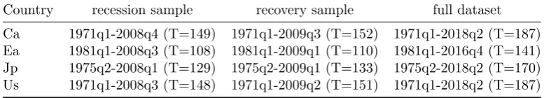
To conclude this work, a short case study on the Great Recession is proposed. The study focuses on four major economies which have been severely impacted by the crisis: Canada, the Euro area, Japan, and the United States. The experiment is conducted on a large 12-variable macroe-conomic model comprising four blocks of variables: a general macroemacroe-conomic block with real gross domestic product (GDP), unemployment rate (UR) and consumer price index (HICP); a monetary policy block with short-term interest rate (STR), long-term interest rate (LTR) and real effective exchange rate (REER); a production block with industrial production (IP), capacity utilization (CU) and total industry employment (TIE); and, for the needs of the ex-ercise, a crisis block with housing starts (HS), a financial stock index (FSI) and the OECD leading composite indicator (LCI) which acts as an overall business cycle indicator. Any series displaying persistence is turned to growth rate to obtain stationarity. The data is quarterly, the sample depending on data availability for each country. It respectively starts in 1971q1 for Canada, 1981q1 for the Euro Area, 1975q2 for Japan and 1971q1 for the United States. The full dataset ends at the end of 2018, but the estimation samples are typically shorter (see below). The data comes primarily from the OECD for Canada, Japan and the United States. For the Euro Area, it is obtained from the Area Wide Model Database of Fagan et al. (2001) which has become the standard for academic research. Financial stock index series come from Bloomberg10.

The aim of the exercise consists in assessing the forecast performances of different models for key phases of the crisis. Figure 2 displays the growth rate of GDP for the four economies over the Great Recession periods. For each country, two critical periods of the crisis are considered. The first is the recession period, the period at which the country enters into negative growth.

10

For Canada, the Euro area, Japan and the United States, this respectively occurs in 2009q1, 2008q4, 2008q2 and 2008q4. The second period considered is the recovery period. It represents the period at which GDP growth starts increasing again, after having reached its minimum. This respectively happens in 2009q4, 2009q2, 2009q2 and 2009q3. These two periods are of special importance for policy makers as they correspond to the beginning of the phases where the crisis initiates and reverts. It is crucial to anticipate them correctly in order to provide an adequate answer to the rapidly changing economic conditions.

2005q1 2005q3 2006q1 2006q3 2007q1 2007q3 2008q1 2008q3 2009q1 2009q3 2010q1 2010q3 2011q1 2011q3 2012q1 2012q3

-8 -4 0 4 8

year-on-year real GDP growth Canada

Euro area Japan United States

Figure 2: Year-on-year GDP growth for the four major economies

The forecasting exercise focuses on predictions from one to eight periods ahead. It is performed in pseudo real time, that is, it does not use information which is not available at the time the forecast is made11. For this reason, for each country and each considered period of the crisis the model is estimated up to the period preceding the beginning of the forecast exercise. To evaluate the performance, two criteria are considered. The first criterion is the classical Root Mean Squared Error (RMSE) which considers the accuracy of point forecasts. Denoting byy˜t+h theh-step ahead prediction and byyt+h the realised value, it is defined as:

RM SEt+h= s

1

h

h

Σ

i=1(˜yt+h−yt+h)

2 ₍₄₉₎

The second criterion is the Continuous Ranked Probability Score (CRPS) of Gneiting and Raftery (2007) which evaluates density forecasts. As pointed by those authors, this criterion presents advantages over alternative density scores such as the log score as it rewards more density points close to the realised value and is less sensitive to outliers. Denoting byF the cumulative

11

distribution function of the h-step ahead forecast density and by yˆt+h and yˆ_t′_+h independent random draws from this density, the CRPS is defined as:

CRP St+h= Z ∞

−∞

(F(x)−✶(x≥yt+h))2dx=E|yˆt+h−yt+h| − 1

2E|yˆt+h−yˆ ′

t+h| (50)

For both criteria, a lower score indicates a better performance.

5.2 Calibration

The forecast exercise considers five competing models. The benchmark is the general time-varying model introduced in section 2 specified with stationary autoregressive processes (Sar) for all the dynamic parameters. Precisely, the dynamic parameters are calibrated by setting

ρi = γi =αi = 0.9 and by using static OLS estimates for the mean terms. The second model considered is the homogenous random walk (Hrw) specification of Primiceri (2005), which obtains from the general time-varying model by setting the autoregressive coefficients of the dynamic processes to one. The third and fourth models respectively consist in the general time-varying model augmented by the random inertia (Ri) and random mean (Rm) extensions developed in section 4. The final model combines the two extensions, thus adding both random inertia and random mean (Rim) to the general time-varying model.

Unlike Primiceri (2005), the priors are not calibrated from a training sample as this strategy wastes a considerable amount of sample information. Rather, simple values are used. For the inverse Wishart priors on the variance-covariance hyperparameters Ωi and Ψi, the degrees of freedom are set to a small value of 5 additional to the parameter dimension, namelyζ0=k+ 5

and ϕ0 = (i−1) + 5. The scale parameters are set to Υ0 = 0.01Ik and Θ0 = 0.01Ii−1.

Similarly, the shape and scale parameters of the inverse Gamma prior distribution on φi are set toκ0 = 5 and ω0 = 0.01. These priors are mildly informative, being sufficiently loose to allow

for a significant degree of time variation in the dynamic parameters, but sufficiently restrictive to avoid implausible behaviours. Finally, the initial period variance scaling terms are set to

τ =µ= ǫ= 5 in order to obtain a variance over the initial periods which is roughly equivalent to that prevailing for the rest of the sample. Estimations are run from 10000 iterations of the MCMC algorithm, discarding the initial 5000 iterations as burn-in sample12.

5.3 Results

With four countries, twelve variables, eight forecast periods and two crisis phases, the full fore-casting exercise consists in 768 forecasts, each of them produced for five competing models. Tables 3 and 4 summarize the results of the experiment13. Table 3 displays the average RMSE and CRPS values for the forecast exercise, while table 4 reports the ratio of these criteria to the benchmark stationary autoregressive formulation. Additionally, Table 4 indicates whether a forecast evaluation criterion is statistically larger (+ entries, for the Hrw model) or smaller (

∗

12

For the sake of illustration, Appendix C displays the stochastic volatility estimates and one-period ahead impulse response functions obtained for the United States with the stationary autoregressive model.

13

RMSE CRPS

Hrw Sar Ri Rm Rim Hrw Sar Ri Rm Rim

Overall (N=768)

Overall 5.03 3.35 2.90 3.28 2.86 14.39 5.00 2.83 4.66 2.76 By country (N=192)

CA 4.00 3.04 2.31 2.87 2.24 8.83 3.78 1.93 2.96 1.92 EA 4.64 2.90 2.57 2.50 2.33 14.69 4.92 2.77 4.10 2.67 JP 6.64 4.23 3.39 4.24 3.45 16.75 5.13 2.99 4.98 3.10 US 4.83 3.22 3.34 3.50 3.41 17.27 6.19 3.63 6.60 3.36

By variable (N=64)

GDP 4.18 2.40 2.00 2.80 2.18 13.13 4.34 2.31 4.17 2.30 UR 1.44 0.78 0.71 0.71 0.71 7.84 2.07 0.95 1.96 0.99 HICP 3.46 2.80 2.68 2.41 2.42 8.02 3.33 2.12 2.78 2.03 STR 2.18 2.47 2.38 2.05 2.27 11.26 4.11 2.36 3.68 2.38 LTR 1.70 1.36 1.19 1.12 1.21 8.68 2.90 1.44 2.69 1.49 REER 3.47 3.18 2.37 2.63 2.23 9.91 3.69 1.94 3.08 1.90 IP 14.31 8.91 7.46 10.04 8.09 34.17 12.46 7.46 12.51 7.49 CU 5.41 3.52 3.04 4.11 3.26 15.21 5.15 2.88 5.29 3.07 TIE 3.84 2.51 2.36 2.36 2.26 12.37 4.56 2.55 4.16 2.43 HS 3.63 2.35 2.28 2.34 2.16 10.26 3.35 1.98 3.00 1.97 FSI 11.32 7.25 6.20 6.37 5.67 24.23 8.96 5.38 8.09 4.72 LCI 5.39 2.63 2.19 2.38 1.85 17.55 5.13 2.60 4.54 2.41

By forecast horizon (N=96)

1q ahead 1.68 1.48 1.39 1.48 1.40 1.40 1.11 1.04 1.13 1.05 2q ahead 2.66 2.17 2.06 2.29 2.12 2.50 1.99 1.79 2.03 1.84 3q ahead 3.53 2.86 2.58 2.93 2.67 3.89 2.69 2.25 2.73 2.32 4q ahead 4.35 3.40 3.07 3.45 3.12 6.36 3.88 2.95 3.81 2.99 5q ahead 5.01 3.76 3.32 3.72 3.29 9.98 4.94 3.23 4.59 3.07 6q ahead 5.90 4.06 3.52 3.95 3.37 16.40 6.36 3.55 5.67 3.31 7q ahead 7.25 4.35 3.62 4.09 3.39 27.45 8.13 3.70 7.34 3.45 8q ahead 9.84 4.70 3.67 4.31 3.49 47.10 10.94 4.13 10.00 4.07

By crisis phase (N=384)

Recession 4.49 3.19 2.90 3.10 2.82 10.58 4.09 2.55 3.98 2.48 Recovery 5.57 3.50 2.91 3.45 2.90 18.19 5.92 3.11 5.35 3.05

RMSE CRPS

Hrw Sar Ri Rm Rim Hrw Sar Ri Rm Rim

Overall (N=768)

Overall 1.50+++ _{- 0.87}∗∗∗ _{0.98 0.85}∗∗∗ _2.87+++ _{- 0.57}∗∗∗ _{0.93 0.55}∗∗∗

By country (N=192)

CA 1.31+++ _{- 0.76}∗∗∗ _{0.94 0.73}∗∗∗ _2.34+++ _{- 0.51}∗∗∗ _0.78∗∗∗ _0.51∗∗∗

EA 1.60+++ - 0.89 0.86∗ 0.81∗∗ 2.98+++ - 0.56∗∗∗ 0.83∗∗ 0.54∗∗∗ JP 1.57+++ _{- 0.80}∗∗ _{1.00 0.82 3.27}+++ _{- 0.58}∗∗∗ _{0.97 0.61}∗∗∗

US 1.50+++ _{- 1.04 1.09 1.06 2.79}+++ _{- 0.59}∗∗∗ _{1.07 0.54}∗∗∗

By variable (N=64)

GDP 1.74+++ - 0.83∗∗ 1.17 0.91 3.03+++ - 0.53∗∗∗ 0.96 0.53∗∗∗ UR 1.84+++ _{- 0.91 0.90 0.90 3.79}+++ _{- 0.46}∗∗∗ _{0.95 0.48}∗∗∗

HICP 1.24++ _{- 0.96 0.86}∗ _0.87∗ _2.41+++ _{- 0.64}∗∗∗ _0.84∗ _0.61∗∗∗

STR 0.88 - 0.96 0.83∗ _{0.92 2.74}+++ _{- 0.57}∗∗∗ _{0.90 0.58}∗∗∗

LTR 1.25 - 0.87 0.82 0.89 2.99+++ - 0.50∗∗∗ 0.93 0.51∗∗∗ REER 1.09 - 0.75∗∗ _0.83∗ _0.70∗∗∗ _2.68+++ _{- 0.53}∗∗∗ _0.83∗ _0.51∗∗∗

IP 1.61+++ _{- 0.84}∗ _{1.13 0.91 2.74}+++ _{- 0.60}∗∗∗ _{1.00 0.60}∗∗∗

CU 1.54+++ - 0.87 1.17 0.93 2.96+++ - 0.56∗∗∗ 1.03 0.60∗∗∗ TIE 1.53+++ _{- 0.94 0.94 0.90 2.71}+++ _{- 0.56}∗∗∗ _{0.91 0.53}∗∗∗

HS 1.54+++ _{- 0.97 1.00 0.92 3.06}+++ _{- 0.59}∗∗∗ _{0.89 0.59}∗∗∗

FSI 1.56+++ _{- 0.85}∗ _0.88∗ _0.78∗∗∗ _2.71+++ _{- 0.60}∗∗∗ _{0.90 0.53}∗∗∗

LCI 2.05+++ - 0.83∗ 0.91 0.70∗∗∗ 3.42+++ - 0.51∗∗∗ 0.89 0.47∗∗∗ By forecast horizon (N=96)

1q ahead 1.14 - 0.94 1.00 0.95 1.26 - 0.93 1.02 0.95 2q ahead 1.23 - 0.95 1.06 0.98 1.26 - 0.90 1.02 0.92 3q ahead 1.23 - 0.90 1.03 0.93 1.45+++ _{- 0.84}∗ _{1.01 0.86}

4q ahead 1.28+ _{- 0.90 1.01 0.92 1.64}+++ _{- 0.76}∗∗ _{0.98 0.77}∗∗

5q ahead 1.33++ _{- 0.88 0.99 0.87 2.02}+++ _{- 0.65}∗∗∗ _{0.93 0.62}∗∗∗

6q ahead 1.45+++ - 0.87 0.97 0.83∗ 2.58+++ - 0.56∗∗∗ 0.89 0.52∗∗∗ 7q ahead 1.67+++ _{- 0.83}∗ _{0.94 0.78}∗∗∗ _3.38+++ _{- 0.46}∗∗∗ _{0.90 0.42}∗∗∗

8q ahead 2.09+++ _{- 0.78}∗∗ _{0.92 0.74}∗∗∗ _4.31+++ _{- 0.38}∗∗∗ _{0.91 0.37}∗∗∗

By crisis phase (N=384)

Recession 1.41+++ - 0.91∗ 0.97 0.88∗∗ 2.59+++ - 0.62∗∗∗ 0.97 0.61∗∗∗ Recovery 1.59+++ _{- 0.83}∗∗∗ _{0.99 0.83}∗∗∗ _3.07+++ _{- 0.52}∗∗∗ _0.90∗ _0.51∗∗∗

Note:

+, ++, +++ : mean RMSE (CRPS)>mean RMSE (CRPS) of Sar model at 10%, 5% and 1% significance level.

∗

∗ ∗

∗ ∗ ∗

A number of conclusions stand. First, the results unambiguously disqualify the homogenous ran-dom walk as the best formulation regarding forecast accuracy. Considering the exercise overall, the Hrw specification produces RMSE which are on average 1.5 times larger than the benchmark Sar model, and CRPS which are on average almost 3 times larger. This indicates that the Sar model represents a considerable improvement over the random walk formulation, the magnitude of the difference being quite large. The difference is also statistically significant at the 1% level, which clears any doubt about the solidity of the conclusion. As additional evidence, the results display similar magnitudes of difference for all the considered sub-specifications, and a vast ma-jority of the differences are statistically significant at the 1% level. This is encouraging as it suggests that the forecast performance is not conditioned on some specific part of the dataset. Finally, note that the Hrw model performs worse in terms of CRPS than in terms of RMSE. This implies that while the random walk performs already poorly in terms of point forecasts, it performs even worse in terms of forecast distributions. In other words, it tends to produce cred-ibility bands which are excessively large compared to the benchmark Sar model, an undesirable feature for any forecast exercise.

Second, the Ri and Rim extensions improve significantly the forecast performances compared to the benchmark Sar model. The achievements of the two extensions prove in fact very close. For the exercise considered overall, they produce a 15% improvement in terms of RMSE, and a 45% improvement in terms of CRPS. The difference is significant at the 1% significance level for both criteria. The gain compared to the benchmark is again quite substantial and provides strong support in favor of the Ri and Rim extensions. It clearly suggests that to optimise forecast performance, it is not sufficient to simply replace the random walk with a stationary specifica-tion. It is further necessary to approach the data generating process underlying the behaviour of the dynamic parameters, which is what is typically achieved by the extensions. Considering the sub-specifications, the Ri and Rim models remain significantly better than the Sar model in terms of CRPS, but not so often in terms of RMSE. Part of the explanation lies in the shorter samples of the sub-specifications, and part in the greater variance of the RMSE criteria. In other words, there remains some variability in the performance of the Ri and Rim in terms of point forecasts compared to the Sar model. In terms of forecast distributions however, these extensions perform consistently better than the Sar benchmark, implying that they typically produce tighter confidence bands.

Third, the Rm model does not perform significantly better than the Sar benchmark. Its per-formances both in terms of RMSE and CRPS look fairly equivalent to those of the Sar model, and prove actually worse on a number of occasions. Also, the difference with the Sar model is hardly ever significant. One likely explanation for this is parsimony. Estimating the mean parameters generates a trade-off between the additional flexibility granted by the extension and the loss of precision implied by the use of additional degrees of freedom. The number of param-eters estimated by the random mean extension can be large (k parameters for eachbi, andi−1 parameters for each di), and it seems that consequently the benefit of the extensions remains moderate. By contrast, the random inertia extension is quite cheap in terms of degree of freedom (one additional parameter per equation only), which may explain its significantly better results.

used together, the gain from approaching the true data generating process exceeds the increased imprecision due to the estimation of the additional parameters. To illustrate this point, Table 5 provides the posterior estimates of key random inertia and random mean parameters for the United States14_:

GDP UR HICP STR LTR REER IP CU TIE HS FSI LCI

ρi 0.48 0.50 0.48 0.49 0.50 0.49 0.58 0.55 0.55 0.52 0.61 0.52

γi 0.99 0.89 0.98 0.99 0.99 0.99 0.88 0.79 0.83 0.99 0.79 0.87

αi - 0.78 0.79 0.84 0.77 0.77 0.78 0.73 0.78 0.78 0.84 0.71

si 0.30 0.02 0.20 0.28 0.07 0.23 0.41 0.01 0.47 0.33 1.16 0.03

ˆ

si 0.52 0.03 0.37 0.49 0.10 0.40 0.59 0.01 0.68 0.52 1.63 0.05

Table 5: Random inertia and random mean estimates for the United States

The first three rows of Table 5 report the posterior estimates for ρi, γi and αi. It appears that the estimates for ρi and αi are considerably smaller than one, about respectively 0.5 and 0.8. Theγi estimates are more ambiguous, taking values comprised between 0.8 and 1. Clearly, a random walk proves inappropriate as it leads to considerably overestimate the amplitude of most autoregressive coefficients. The stationary autoregressive model usingρi =γi =αi = 0.9 represents some improvement, but still creates a considerable gap with the values supported by the data. The results also confirm the relevance of a formulation equation by equation as considerable differences arise between different variables. For instance, the γi coefficients on GDP, STR, LTR and REER are at 0.99 against much lower values of 0.79 for CU and FSI. The last two rows of Table 5 respectively present the random mean posterior estimates si, and for the sake of comparison the OLS estimatessˆi used as hyperparameters in the stationary autore-gressive model. Remember that these coefficients represent the long-run equilibrium value for the residual volatility of the model, and that a random walk formulation amounts to assuming

si= 1. Again, it is not difficult to see that a random walk leads to considerably overestimate the amplitude of the stochastic volatility component. The OLS estimates used for the Sar model are already significantly lower and thus represent an improvement, but the si values endogenously estimated by random mean turn out to be even lower.

The fourth and final conclusion about the crisis experiment is that the best forecasting model between the Ri and Rim specifications depends on the forecast horizon. At short horizon (one to four quarters), the pure Ri model performs slightly but consistently better than its Rim counterpart. At longer horizon (five to eight quarters) the relation is reversed and the Rim model becomes the leading model. This comes as another illustration of the trade-off between greater flexibility and increased imprecision. At short forecast horizons, the Rim model is too costly in terms of parameters and the simple, more parsimonious Ri model performs better. At longer horizons, it becomes crucial to approach the true data generating process to produce accurate predictions and the more flexible Rim model dominates.

14

6

Conclusion

This paper introduces a new general time-varying VAR model which adopts a full equation-specific approach. It provides general autoregressive formulations for the dynamic parameters, in contrast to the random walk assumption used by the canonical approach of Primiceri (2005). On the methodological side, it shows that the efficiency of the precision sampler developed by Chan and Eisenstat (2018) crucially depends on the dimension of the dynamic parameter con-sidered. Based on this conclusion, it proposes an optimal sampling algorithm which maximizes the efficiency of the estimation procedure.