On the Identification of Technology Shocks: An Alternative
to the Standard Long-Run Method
Ufuk Devrim Demirel
Department of Economics, University of Colorado, Boulder, USA Email: [email protected]
Received September 11, 2012; revised October 13, 2012; accepted November 15, 2012
ABSTRACT
This study proposes an alternative procedure to identify technology shocks using vector autoregressions (VARs). The proposed procedure delivers improved small-sample properties relative to the standard long-run identification method provided that the dynamics of the observed variables can only be captured precisely by an infinite-order VAR. Monte Carlo experiments on artificial data produced by a standard version of the real business cycle model demonstrate that the proposed procedure is associated with smaller average bias and mean square error. These results obtain under a range of specifications regarding the share of technology shocks in overall output variability.
Keywords: Technology Shocks; Long-Run Restrictions; Relative Identification
1. Introduction
In the real business cycle (RBC) literature, technology shocks are frequently identified by implementing long-run restrictions in structural vector-autoregressions (VARs) (see, e.g. [1-3]). A number of recent studies have called into question the plausibility of identifying technology shocks by imposing long-run restrictions on VARs. Demirel [4], Mertens [5], and Chari et al. [6] find that the standard long-run identification approach can be highly inaccurate if the number of lags included into the esti-mated VAR is smaller than the number of lags involved with the actual data-generating process. Since in many RBC models the reduced-form dynamics of the observed variables can only be captured by an infinite-order VAR, this type of mismatch between the estimated and actual lag structures is often relevant (see [6-9]). In this paper, I propose an alternative identification procedure that is designed to reduce the lag-truncation bias that emerges in the presence of this mismatch. I show that, in the estima-tion of the impact response of labor to a technology shock, the proposed procedure is associated with smaller average bias and mean square error relative to the stan-dard long-run identification method.
To implement long-run restrictions in structural VARs, one needs an estimate for the zero-frequency spectral density of the data. Christiano et al. [10,11] show that the standard long-run method uses a particular estimate of the zero-frequency density that is based on the OLS es- timate of the sum of VAR coefficients. In the presence of a lag-truncation-type mismatch between the estimated
and actual VARs, the OLS-based estimate of the sum of VAR coefficients can be highly biased. Christiano et al. [10] argue that the poor performance of the standard long-run identification procedure is primarily due to this bias involved with the OLS estimate of the sum of VAR coefficients and suggest considering non-parametric me- thods to estimate the zero-frequency spectral density of the data. Using Monte Carlo simulations, they find that their non-parametric procedure (henceforth, the CEV method) outperforms the standard OLS-based long-run identification scheme under some reasonable parame- terizations of the RBC model.
ployment. The proposed procedure selects the shock that drives as much as possible of the long-run variation of labor productivity while explaining as least as possible of the short-run variation. In this sense, it is expected to counteract the tendency of the standard method to deliver a shock that overshoots the short-run variability of the VAR variables. Following Uhlig [12], I use principal components analysis to determine the shock that satisfies this property.
Using Monte Carlo simulations, I evaluate the per- formance of the proposed method relative to the standard long-run and the CEV procedures. In a series of simula- tion experiments, I produce artificial data sequences us- ing the most commonly adopted parameterizations of the RBC model. Then, I apply the proposed procedure as well as the standard long-run and the CEV methods to each simulated data sequence to recover technology shocks. I consider two different VAR specifications in which hours worked is entered into the VAR in first differences and in levels. I find that, in the estimation of the con-temporaneous response of labor to a technology shock, the proposed method outperforms the standard long-run and the CEV methods in terms of average bias and mean square error.
The remainder of the paper is organized as follows: Section 2 discusses the identification procedures based on long-run restrictions. Section 3 outlines the proposed method and describes its implementation. Section 4 eva- luates the performance of the proposed approach rela- tive to the standard long-run and the CEV method using Monte Carlo simulations. Section 5 summarizes the main results and concludes.
2. Identifying Technology Shocks with
Long-Run Restrictions
2.1. The Standard Long-Run Method
As discussed in Gali [13], in a large class of real business cycle (RBC) models, long-run variability of labor pro-ductivity is exclusively driven by technology shocks. This distinguishing property is referred to as the exclusion res- triction. Furthermore, in the standard RBC framework, the impact of a positive technology shock on labor pro-ductivity is positive in the long-run. This property, in turn, implies a sign restriction. Exclusion and sign restrictions can be exploited to identify technology shocks using a VAR(m) specification of the form
1t t
Y A L Y ut (1) where
11
m i i i
A L A L
(2)and
e vector Yt is often specified as
1 1
t t Eu u .
Th
log 1 log
t t t
Y y l L lt
log y lt t
and
1L
loglt ty andquasi-where respectively de-
erage labor pro di
note av ductivi fferenced per-
capita hours. Note that, in the case 0, aggregate employment enters Yt in levels. This is pecification
adopted by many udies including Christiano et al. [10,11], and will be among the cases I consider in the following analysis. Another common practice is to in- clude the first-difference of aggregate employment into the VAR specification (by setting 1
the s st
). As shown by Chari et al. [6], in the case 1, uced-form VAR representation for Yt ceases ist in the RBC model.
To circumvent this oblem, they set the quasi differenc- ing parameter to 0.99. In this case, Yt admits an
infi-nite-order VAR representation and the impulse response of labor productivity to a technology shock is indistin-guishable from the case 1
a red to ex pr
. I will also consider the case 0.99 in the foll analysis.
Give Yt can be expressed in m
owing
n (1), oving average
fo
(3) where
rm as follows:
t t
Y B L u
1
n n
.B L I A L L tor of structural disturbance
The mapping from
the vec s, t
,
to the vector ofVAR innovations, ut, is conjectured t be of the form
t t
u R
o
(4) where E t1 t 1 Inn. Without loss of generality, the
technology shock can be assumed to rank first in t. To evaluate the effects of a technology shock on one
needs to know t
Y,
A A1, 2, , Am
as well as the first col- umn of the mat ill be denoted R1. Thevector R1 describes the contemporaneous effec of a technology shock on Yt and is often referred to as the
impact vector. The objects
1, 2, , m
rix R, which wts
A A A and Ω are typically estimated using OLS R1, however,
one needs to impose exclusion and sign restri ions. Define
. To estimate ct
1
1G B R. Given that the first element of
t
is the ck, exclusion and sign restrict- ns imply that
technology sho
tio G
1 is of the form0
g
11 1 11
1
# #
m
n i
i
G B R
(5)where g110 and the upper-right expression is a
n1
dimensional row vector of zeros. The form de-by (5) implies that only technology shocks can influence labor productivity (the first element in Yt) in
the long-run. The object G
1 can be identified ing the zero-frequency spectra nsity matrix of Yt. Thestandard long-run procedure uses the OLS estim es for scribed
us
t l de
density of a
1
1 . (6) Once is estimated using (6),
identified as t
.
Note that there are many ways in which the matrix
how that the
Then, using the estimate for
t Y S
0
Y
h
ition s
OL
1
0 1
Y n n n n
S I A I A
OLS Se ma
1
G
S as can be
trix that factors SY
0OL
1 1 Y
0
G G S OLS
0OLSY can be decomposed in the form PP
. Yet, Christiano et al. [11] s
of this form that are also consistent with the structure described by (5) all have the same first column. Therefore, a lower-triangular Cholesky decom- position can be applied to SY
0 OLS to obtain the esti- mateS
0OLSY S
decompos s
1 chol
Y
0 OLS
G S .
1G
1
R
, ecove
and the relationship
(7) where
1
1 n n
1G B RI A the impact vector of
red as
1 1 chol 0
OLS
R I I A S
the technology shock can be r
n
1 1
OLS
n n n Y
1 1
I is
2.2. A Non-Parametric
a vector of all zeros but the 1st
Alternative to the
The thod is known to deliver im-
1n
with element is replaced unity.Standard Method
standard long-run me
precise estimates in the presence of VAR misspecifi- cation. Christiano et al. [10] argue that this is because the OLS-based estimate of the zero-frequency spectral den- sity of Yt (given by 6) becomes highly inaccurate if the data-generating process is an infinite-order VAR. To remedy this problem, they suggest adopting a nonpara- metric approach to estimate the zero-frequency spectral density. In particular, they consider a Bartlett estimate of the form
1
1 1
1 0 NP T T
Y t t k
k T t k
S g k Y Y
T
(8)where
1 if0 if otherwise.
k r k r g k
The pr ure of Christiano et al. [10] involves re- pl
oced
acing SY
0OLS with
0NP Y
S and identifying the
impact v techno ck as
1
NP I A S ector of the
R I
zati
logy sho
1 1 1 chol 0 .
NP
n n n Y
(9)Christiano et al. [10] show that, under certain rele parameteri ons of the RBC model, the non-parametric
m
vant
ethod (henceforth, CEV procedure) proves more suc- cessful relative to the standard method1. This is because,
0 NPY
S accounts for some of the information SY
0OLS is unable to capture due to lag-truncation and provides acurate estimate of the zero-frequenc l density. However, Mertens [5] shows that the CEV pro-cedure (fully described by 9) fails to properly utilize this additional information in the estimation of the impact vector. Consequently, the improved small-sample results of the CEV method do not extend to a wider range of parameterizations of the RBC model.
3. Relative Identification
more ac y spectra
posed identification approach, I next uences of implementing the standard 3.1. Motivation
To motive the pro discuss the conseq
long-run identification procedure in the presence of VAR misspecification. Suppose that the true data-generating process is an infinite-order VAR of the form
1t t t
Y F L Y v (10)
where
11
,
i i i F L F L
and Ev vt1 t 1 with a finite-order
. Note that any attempt to estimate (10) VAR of the form (1) will always re- sult in a lag-truncation bias. Christiano et al. [10] show that the residual covariance matrix of the misspecified
VAR is related to the true residual covariance ma- trix
through the following relationship:1
π
i i
, ,
1
min e
2π
m Y
A A D S D
π
e d
(11 where
)
e i ei eD F A i ,
and F
ei , A
ei denote the lag polynomials
F L , A L
evaluated at ei,
. This equality follows
imme ctral domain representations of
d (1 According to (11) the OLS procedure se- lects the autoregressive matrices
1, 2, , m
diately from n 0).
the spe (1) a
A A A to minimize a quadratic form that measures the distance between the actual and fitted lag polynomials averaged across all frequencies weighted by the spectral density of
t Y
Y i.e. S at each frequency.
Equation (11) highlights two major consequences of sspecified VAR: 1—
adopting a mi In the presence of a
la
on
single- ha
dentifying restric- tio
fraction of the infi- ni
forecast revision variances of ployment as
g-truncation problem, the OLS procedure cannot be expected to deliver an accurate estimate for the sum of VAR coefficients unless the spectral density of Yt at
zero frequency is large relative to non-zero frequencies. Thus, in general, we have A
1 F
1 . 2—Equation 11) also implies that 0, i.e.,
is a positive semi-definite matrix. Thu tes A
1 and Ωare both biased under isspecification.
The main motivation for relative identification emerges upon an investigation of the implications of these biases
(
s, the estima R m
VA
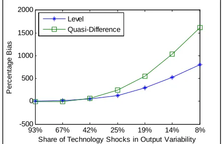
the short-run variances of labor productivity and aggre- gate employment the technology shock is found to drive using the standard long-run identification method. Figure 1 displays the percentage difference between the cur-rent-period forecast error variances the technology shock is estimated to explain in the artificial data (averaged across 1000 trials) and the true fraction the technology shock explains in the RBC model. It is observed that the shock identified using the standard long-run method overestimates the true values. This finding obtains under alternative scenarios regarding the share of technology shocks in overall output variability2. In all considered
cases, the shock the standard long-run method yields overshoots the true fraction of short-run variances the technology shock explains in the RBC model. As Figure 2 attests, similar patterns obtain under the parameteriza- tion of the RBC model adopted by Chari et al. [6].
As discussed in the previous section, the standard long-run approach determines the disturbance that
ndedly explains all of the infinite-period-ahead fore-cast revision variance of labor productivity. Demirel [4] shows that this is equivalent to determining the shock that explains on its own as much as possible of the long-run variance of labor productivity. Thus, the stan-dard long-run identification procedure can be viewed as a version of the maximum share approach suggested by Francis et al. [15] and implemented in the frequency domain by DiCecio and Owyang [16].
Monte Carlo experiments reveal that, in the presence of lag-truncation bias, imposing this i
n on the misspecified VAR yields a shock that tends to explain too much of the current-period forecast error variance of labor productivity and employment relative to the true technology shock.
To counter this tendency, I propose considering the disturbance for which the explained
te-period-ahead forecast variance of labor productivity is as great as possible relative to the explained fractions of the current-period forecast variances of labor produc- tivity and employment. This procedure involves deter- mining the disturbance for which the difference be-
tween the explained fractions of long-run and shortrun variances reaches a maximum. Thus, the procedure places a certain amount of weight on minimizing the current- period forecast revision variance the identified shock explains.Although this property does not perfectly over-lap with the notion of a technology shock, in the presence of lag-truncation bias, the proposed adjustment to the long-run identifying assumption works against the ten-dency of the standard approach to overshoot the true short-run variances. This, in turn, results in a more accu-rate estimate for technology shocks.
3.2. Implementation
Define k-period-ahead labor productivity and em
k var Etlog
yt k lt k
Et1log
y l
,
var log
1log
.t k t k
t t k t t k
k E l E l
Using (1) and (4), infinite-period-ahead forecast revi- sion variance of labor productivity can be found as
91% 62% 37% 22% 15% 10% 9%
-500 0 500 1000 1500 2000 2500
Level
Quasi-Difference
Share of Technology Shocks in Output Variability
P
er
c
en
tage
B
[image:4.595.311.534.351.503.2]ias
Figure 1. Standard long-run method’s bias profile in the estimation of short-run variances under the parameteriza- tion of Christiano et al. [11].
93% 67% 42% 25% 19% 14% 8%
-500 0 500 1000 1500 2000
Share of Technology Shocks in Output Variability
Pe
rc
e
n
ta
g
e
Bi
a
s
Level
Quasi-Difference
Figure 2. Standard long-run method’s bias profile in the estimation of short-run variances under the parameteriz tion of Chari et al. [6].
2Output variance in these experiments is computed using simu-lated band-pass filtered data sequences of length 50,000 quar-ters.
[image:4.595.312.534.552.696.2]
1
11 1
lim I n 1 t t 1 n k k L RE R L I
(12)
where L
1 In n A
11 and I1in is a
1n
n vari- vector of all zeros but the ithSimilarly, current-perio
elem rep
.
(13)
Using
expressions (12) and (13) and can be rewritten as
(14)
where
and . Expression (14) shows how
sion variance of labor pro- ent is laced with
unity. d forecast revisio
ances of labor productivity and aggregate employment can be respectively expressed as
1
11 1
0 I REn t t R In ,
2
21 1
0 I REn t t R In
1
11
,
n i i
t t n n n n
i
E I I I
1 i 1 i
k i k i
1
lim lim , 0 0 ,
0 0 ,
n n n i i k k
1 11 1 1 1
1 1
1 1 1 1
2 2
1 1 1 1
1 1 ,
0 ,
0 ,
i i
n n n n
i i
n n n n
i
i i
n n n n
i
k I T RI I R T I
I RI I R I
I RI I R I
lim k
11 n n 1
T I infinite-period forecast revi
vity and current-perio
ducti d forecast revision variances
of labor productivity and employment can be decom- posed into n elements each exclusively attributable to a particular structural disturbance in
ε
t. Since the first ele-ment in
ε
t corresponds to the technology shock, its con-tribution to the infinite-period forecast variance of
log y lt t is given by klim
k 1. Similarly, the con-tribution of the technology shock to the current-period forecast vision variances of re log
y lt t
and log
lt are, respectively,
0 1 and
0 1. Now, let’s define
,i klim k i i i .
0
0
After obtaining estimates for the objects
1be im r-tria
and , relative identification procedure can ple-
me lar
nted as follows: Let P correspond to a lowe ngu- Cholesky decomposition of Ω (i.e., PP). Given an orthonormal matrix Q (i.e., QQ n n ), a particular
decomposition of the covariance matrix Ω ca be ob- tained via the relationship
n
HH
where H PQ. Also note that one can write QQ
iQ Qi iwhere Qidenotes the ith column vector of Q. It is shown in the
appendix that the statistic ,i
22
can be d as
where
expresse
1 11
1,
11
1 1
1 1
i i n n n n n n i
i n n i i n n i
Q P I A I I A PQ
Q P PQ Q P PQ
(15)
1ij
n n is a
n n
maent is re es determin
trix of all zeros bu
ith-col placed with unity.
tive id ion ing the decomposi-
d as
t the Rela- umn jth
entificat the
-row elem involv
nce m
tion of covaria atrix PQQ P indexed by the Q for which the first column Q1 results in the maxi- mum value (15) can achieve. Thus, the associated identi- fication problem can be expresse
1 1 1
max
Q Q Q (16) subject to
11 0
A PQ
1 1 1 1 and 1
Q Q InIn n
11
1 1n n
where, as suggested by (15),
The first constraint
1
11 .
n n n n
P I A I A
11 22
1n n 1n n P P P P
P
1
al m an
g-r o
A
1 1
Q Q
atrix un effect ositive.
ensures that be- longs to an orthonorm d the second c
guarantees that the lon f the identifi hock on 1 Q o ed s g nstraint
labor productivity is p s shown in Uhli [12], the optimal value of Q1 (denoted Q1
) that solves (16)
is given by the eigenvector of Λ that corresponds to its greatest eigenvalue, i.e., the first principal component of
Λ. Once Q1
is recov d by solving r the first prince-
pal component of Λ, the impact vector of the technology shock can be estimated as
1 1.
REL
R PQ (17) Throughout the rest of t
ere fo
he an ies of
of t
alysis, we shall compare the small-sample propert th
scribed by (17) with those he th
I exercises. In these using the baseline e relative method de- standard long-run and e CEV methods respectively described by (7) and (9).
4. Monte Carlo Experiments
To evaluate the performance of the proposed method, next conduct a series of simulation
experiments, I produce artificial data
RBC model adopted by Chari et al. [6] and Christiano et al. [11]. Since the model is standard, I shall skip the ex- planation of the full theoretical structure. It should how- ever be noted that, in the standard RBC model, the equi- librium dynamics of the vector
log 1 log
t t t t
Y y l L l
can only be described accurately by an infinite-order VAR. Thus, using a finite-order VAR to id ntify tech- nology shocks will always result in a lag-trun n bias,
which will play a central role in the following experi- ments.
I consider two alternative parameterizations of the RBC model adopted by [6] and [11]3. These parameter
choices render the results of the analysis immediately comparable with the results of the previous studies. In addition, I consider a range of scenarios regarding the share of technology shocks in overall output variability. Following the rest of the literature, for each alternative specification, I simulate 1000 data sequences each of length T = 240 quarters. Then, I run a VAR with 4 lags on each of these 1000 data series and identify technology shocks using the proposed method as well as the standard long-run and the CEV methods. In all exercises, I esti- mate a bivariate VAR of the form
associated with each method in the estimation of the impact coef ient of la- bor. The impact coefficient of labor corresp s to the co
asi- di
increases. As the share of technology shocks be- co
. [6] for level and quasi- di
log 1 log
t t t t
Y y l L l .
First, I focus on the average bias
fic ond
ntemporaneous percentage response of employment to a one-standard-deviation technology shock. Average bias is defined as the percentage difference between the true impact coefficient in the RBC model and the average of all estimated impact coefficients across simulations.
Figures 3 and 4 display the bias profile of each identi-fication method under the parameterizations of Chris-tiano et al. [11] and Chari et al. [6] for level and qu
fference specifications. Observe that the average bias associated with the relative identification method is much smaller compared to the other methods in all considered cases.
The standard long-run method becomes more accurate as the share of technology shocks in overall output vari- ability
mes smaller, the standard method turns less accurate. This does not appear to be the case for the CEV method. Compared to the relative method, however, the CEV method proves less successful.
Figures 5 and 6 demonstrate the root mean square er-ror profiles under the parameterizations adopted by Chris- tiano et al. [11] and Chari et al
fference specifications. Root mean square error statistic measures average bias and sampling uncertainty simul-taneously. It is defined as
1000
21
1 1000
i xixwhere xi denotes the impact coefficient estimate obtained
from the ith experiment and x is the true lue of the im-
pact coefficient.
-run and CEV procedures. This appears to
va
Observe that the relative method is also associated
with significantly smaller mean square error compared to the standard long
be the case for all considered parameterizations and volatility specifications.
93% 67% 42% 25% 19% 14% 8%
-200 0 200 400 600
Share of Technology Shocks in Output Variability
P
er
c
ent
age B
ias
Level Specification
Relative Bartlett Standard
(a)
93% 67% 42% 25% 19% 14% 8%
-1000 -800 -600 -400 -200 0
Share of Technology Shocks in Output Variability
P
erc
ent
age B
ias
Quasi-Difference Specification
Relative
Bartlett
Standard
[image:6.595.333.508.450.722.2](b)
Figure 3. Bias profiles under the parameterization of [11].
91% 62% 37% 22% 15% 10% 9%
-200 0 200 400 600 800
Share of Technology Shocks in Output Variability
P
e
rc
en
ta
ge
B
ias
Level Specification Relative
Bartlett Standard
(a)
91% 62% 37% 22% 15% 10% 9%
-1200 -1000 -800 -600 -400 -200 0
Share of Technology Shocks in Output Variability
P
er
c
ent
a
ge B
ia
s
Quasi-Difference Specification
Relative Bartlett Standard
(b)
Figure 4. Bias profiles under the parameterization of [6]. 3See Chari et al. [6] and Christiano et al. [11] (or Demirel [4])
93%0 67% 42% 25% 19% 14% 8% 0.5
1 1.5 2
Share of Technology Shocks in Output Variability
S
qua
re
R
oo
t of
M
ea
n S
q
uar
e
E
rr
or
Level Specification Relative
Standard Bartlett
(a)
93%0 67% 42% 25% 19% 14% 8%
0.5 1 1.5 2 2.5
Share of Technology Shocks in Output Variability
S
qua
re
R
oo
t of
M
ea
n S
q
uar
e
E
rr
or
Quasi-Difference Specification Relative Standard Bartlett
[image:7.595.83.262.84.373.2](b)
Figure 5. Mean square error profiles under level and quasi- difference specifications (parameterization of [11]).
91%0 62% 37% 22% 15% 10% 9%
0.5 1 1.5 2 2.5
Share of Technology Shocks in Output Variability
S
qu
ar
e R
o
ot
of
M
ean
S
qu
ar
e E
rr
or
Level Specification Relative
Standard Bartlett
(a)
91%0 62% 37% 22% 15% 10% 9%
0.5 1 1.5 2 2.5 3
Share of Technology Shocks in Output Variability
S
q
uar
e
R
o
ot
of
M
ea
n S
q
ua
re E
rr
o
r
Quasi-Difference Specification Relative
Standard Bartlett
(b)
Figure 6. Mean square error profiles under level and quasi- difference specifications (parameterization of [6]).
5. Concluding Remarks
This study suggests an alternative approach to identify technology shocks using VARs. I test the performance of the proposed method by applying it to artificial data gen- erated by the standard RBC model. I evaluate the small- sample performance of the proposed procedure by re- covering technology shocks from simulated time-series data that are produced by a standard version of the RBC model. I consider alternative parameterizations of the RBC model as well as a range of specifications regarding the share of technology shocks in overall output va abil- ity. Monte Carlo experime on simulated data reveal
un iden- e literature and its d by [11]. In particular, it
ri nts
that the proposed method delivers considerably improved small-sample properties than the standard long-r
tification method widely adopted in th non-parametric version propose
significantly reduces the average bias and mean square error in the estimation of the impact coefficient of labor.
It is important to note that this study assesses the small-sample properties of the proposed relative identi- fication approach for a specific range of data-generating processes. Since the small-sample performance of an estimation procedure depends on the properties of the underlying data-generating process, one should be cau- tious generalizing the results. At the very least, the find- ings suggest that the relative approach can identify tech- nology shocks far more accurately provided that the data-generating process is the standard RBC model.
REFERENCES
[1] N. Francis and V. A. Ramey, “Is the Technology-Driven Real Business Cycle Hypothesis Dead? Shocks and Ag-gregate Fluctuations Revisited,” Journal of Monetary Economics, Vol. 52, No. 8, 2005, pp. 1379-1399.
doi:10.1016/j.jmoneco.2004.08.009
[2] N. Francis and V. A. Ramey, “Measures of Per Capita Hours and Their Implications for the Technology-Hours Debate,” Journal of Money, Credit and Banking, Vol. 41, No. 6, 2009, pp. 1071-1097.
doi:10.1111/j.1538-4616.2009.00247.x
[3] J. Gali and P. Rabanal, “Technology Shocks and Aggre-gate Fluctuations: How Well Does the RBC Model Fit Postwar US Data?” NBER Macroeconomics Annual, Vol. 19, 2004, pp. 225-288.
[4] U. D. Demirel, “Identification of Technology Shocks Using
Misspecified Colorado, Boulder,
2012.
VARs,” University of
[5] E. Mertens, “Are Spectral Estimators Useful for Imple-menting Long-Run Restrictions in SVARs?” Journal of Economic Dynamics and Control, Vol. 36, No. 12, 2012, pp. 1831-1842. doi:10.1016/j.jedc.2012.06.007
[image:7.595.84.265.415.711.2]9.010 doi:10.1016/j.jmoneco.2008.0
“Can Long-Run [7] C. J. Erceg, L. Guerrieri and C. Gust,
Restrictions Identify Technology Shocks?” Journal of the European Economic Association, Vol. 3, No. 6, 2005, pp. 1237-1278. doi:10.1162/154247605775012860
[8] F. Ravenna, “Vector Autoregressions and Reduced Form
1016/j.jmoneco.2006.09.002
Representations of DSGE Models,” Journal of Monetary Economics, Vol. 54, No. 7, 2007, pp. 2048-2064.
doi:10.
[9] T. F. Cooley and M. Dywer, “Business Cycle Analysis without Much Theory: A Look at Structural VARs,” Journal of Econometrics, Vol. 83, No. 1-2, 1998, pp. 57- 88. doi:10.1016/S0304-4076(97)00065-1
[10] L. Christiano, M. Eichenbaum and R. Vigfusson, “Alter-native Procedures for Estimating Vector Autoregressions Identified with Long-Run Restrictions,” Journal of the European Economic Association, Vol. 4, No. 2-3, 20 pp. 475-483. doi:10.1162/jeea.2006.4.2-3.475 05,
mboldt Univer-nual, Vol. 21, 2006, pp. 1-72.
[12] H. Uhlig, “What Moves Real GNP?” Hu sity, Berlin, 2003.
[13] J. Gali, “Technology, Employment, and the Business Cy- cle: Do Technology Shocks Explain Aggregate Fluctua-tions?” American Economic Review, Vol. 89, No. 1, 1999, pp. 249-271. doi:10.1257/aer.89.1.249
[14] D. W. K. Andrews and J. C. Monahan, “An Improved Heteroskedasticity and Autocorrelation Consistent Co-variance Matrix Estimator,” Econometrica, Vol. 60, No. 4, 1992, pp. 953-966. doi:10.2307/2951574
[15] N. Francis, M. T. O
[11] L. Christiano, M. Eichenbaum and R. Vigfusson, “As-sessing Structural VARs,” NBER Macroeconomics
An-wyang, J. E. Roush and R. DiCecio,
by (1) we have
2) can be rewritten as
(18)
productivity and ag- gregate employment can be respectively written as
,
Now using (18) and (19), the statistic can be ob- tained as
Let
“A Flexible Finite-Horizon Alternative to Long-Run Re-strictions with an Application to Technology Shocks,” Federal Reserve Bank of St. Louis Working Paper 2005- 024F, 2010.
[16] R. DiCecio and M. T. Owyang, “Identifying Technology Shocks in the Frequency Domain,” Federal Reserve Bank of St. Louis Working Paper 2010-025A, 2010.
Appendix
In the reduced-form VAR described
1 2
0 1 n
1 I P1n
Q Q P Ii i 1n2
1 1
1
0 .
i n
n i i n
i
I P Q Q P I
(19) RR PQQ P
. Thus, the infinite-period-ahead fore- cast revision variance of labor productivity described by (1
,i
1
11 1
lim n 1 1 n
n i
k I L PQQ P L I
k
1 1
1 1
1
1 1 ,
n i i n
I L P Q Q P L I
where l
1 In n A
11. Similarly, current-period forecast revision variances of labor
1 1
, 1 1
1 1 2 2
1 1 1 1
1 1
i n i i n
n i i n n i i n
I L PQ Q P L I
I PQ Q P I I PQ Q P
I
(20)
11
1n n denote a
n n
matrix of all zeros but theith
e reexpressed as
which brings us to (15) in the text.
-column jth-row element is replaced with unity. Then,
(20) can b
11 11
11
11 22 ,i trace 1n nL 1 PQ Q P Li i 1 1n nPQ Qi i n n i iP Q P Li 1 1n nL 1 PQi Q Pi 1n nPQi Q Pi 1n n
P 122 PQ Q ,
![Figure 3. Bias profiles under the parameterization of [11].](https://thumb-us.123doks.com/thumbv2/123dok_us/52911.505532/6.595.333.508.450.722/figure-bias-profiles-parameterization.webp)
![Figure 5. Mean square error profiles under level and quasi- difference specifications (parameterization of [11])](https://thumb-us.123doks.com/thumbv2/123dok_us/52911.505532/7.595.84.265.415.711/figure-mean-square-error-profiles-difference-specifications-parameterization.webp)
