Munich Personal RePEc Archive
Sentiment indicators and macroeconomic
data as drivers for low-frequency stock
market volatility
Lindblad, Annika
University of Helsinki
19 July 2017
Sentiment indicators and macroeconomic data as drivers for
low-frequency stock market volatility
∗Annika Lindblad†
July 19, 2017
Abstract
I use the GARCH-MIDAS framework of Engle et al. (2013) to examine the relationship between the macro economy and stock market volatility, focusing on the role played by survey-based sentiment indicators compared to macroeconomic variables. I find that once the information in sentiment indicators is controlled for, backward-looking macroe-conomic data does not include useful information for predicting stock return volatility. On the other hand, forward-looking macroeconomic variables remain useful for forecast-ing stock market volatility after sentiment data is taken into account. The term spread is the best predictor for stock return volatility over long horizons.
JEL Classification: G17, G12, C53
Keywords: stock market volatility, volatility components, MIDAS, survey data, macro finance link
∗I thank Markku Lanne and Matthijs Lof, as well as the participants of the FDPE Econometrics Workshops
and the SoFiE 2016 Summer school, for useful suggestions and comments. I gratefully acknowledge financial
support from the OP Group Research Foundation, the Yrjö Jahnsson Foundation and the Academy of Finland.
†Department of Political and Economic Studies and HECER, University of Helsinki, Finland. E-mail:
1 Introduction
Stock market volatility is crucial for asset allocation and risk management, and it can also
be interpreted as a measure of risk and uncertainty. Therefore, it is important to understand,
model and forecast stock return volatility accurately. While short-term volatility (e.g., daily)
is well described and forecasted by, for example, GARCH models and stochastic volatility
models1
, longer horizon modelling and forecasting of volatility (e.g., monthly or quarterly)
relies on, for example, autoregressive models for realised volatility, predictive regressions and
component GARCH models. It is well established by, for example, Fama and French (1989)
and Schwert (1989a), that risk premiums and stock market volatility are countercyclical. The
research on the macroeconomic determinants of stock market volatility has its roots in Schwert
(1989b) and Officer (1973), but much of the early literature found links that are weaker than
expected. The recent financial crisis underlined the importance of understanding the sources
of volatility, leading to new interest in determining how the macroeconomy affects financial
market volatility. For example, component GARCH models – where volatility is decomposed
into a transitory high-frequency component and a slowly evolving low-frequency component
– have recently provided robust evidence in favour of macroeconomic determinants of
(low-frequency) financial market volatility.2
Knowledge of the macroeconomic variables affecting
volatility improves our understanding of why volatility varies over longer time periods and
can enable more precise volatility forecasts, especially over long horizons.
The main aim of this paper is to compare the information content of macroeconomic
fundamentals and survey-based sentiment data for stock return volatility in the
GARCH-MIDAS3
framework of Engle et al. (2013). The GARCH-MIDAS model decomposes volatility
into two components: a short-term (GARCH) component (e.g., daily frequency) which
fluc-tuates around a long-term trend (e.g., quarterly frequency). The low-frequency component of
volatility is directly determined by macroeconomic variables. It is clear from earlier research4
that there is a vast number of potentially good explanatory variables for stock market
volatil-ity. The GARCH-MIDAS literature has found a large set of useful predictors by including
1See, for example, Poon and Granger (2003) for a survey, or Andersen et al. (2006) for an overview of
volatility forecasting.
2For example, Engle and Rangel (2008), Engle et al. (2013) and Conrad and Loch (2014).
3GARCH-MIDAS stands for a generalised autoregressive conditional heteroskedasticity (GARCH) model,
combined with a mixed data sampling (MIDAS) approach, see Section 3 for details.
4For example, Christiansen et al. (2012) and Conrad and Loch (2014). See Section 2 for details.
one variable at a time (or the level and volatility of the same variable) into the MIDAS
poly-nomial.5
I focus on models containing different types of variables in order to investigate how
including survey-based sentiment data affects the explanatory power of macroeconomic data.
I determine whether the in-sample fit and the out-of-sample forecasting ability of
GARCH-MIDAS models can be improved by combining information in the two types of indicators. This
paper builds on Engle et al. (2013), who introduced the GARCH-MIDAS model, and Conrad
and Loch (2014), who, using the GARCH-MIDAS framework, found many macroeconomic
and sentiment variables useful for modelling long-term stock market volatility.
First, I establish a baseline using GARCH-MIDAS models driven by one variable at a
time.6
Contrary to earlier literature, I use a real-time macroeconomic data set to match the
information sets of the agents at the time and accurately take into account data revisions. I
also argue that the recession probabilities given by professional forecasters – a novel measure
in this context – proxy the business cycle, making them interesting predictors for stock return
volatility. Principal components based on the macroeconomic and sentiment data are used to
infer the usefulness of summarising information in the variables.
Next, I determine the relative and combined importance of macroeconomic data and
sentiment indicators as drivers of long-term stock return volatility by including different
types of variables simultaneously in the GARCH-MIDAS model. These results are compared
to the baseline obtained earlier. This allows us to infer the marginal benefit for the in-sample
fit from adding a second variable into the model.
Finally, I explore the out-of-sample forecasting performance of the GARCH-MIDAS
spec-ifications in order to determine whether stock return volatility forecasts can be improved by
simultaneously utilising information in macroeconomic variables and survey-based sentiment
data. I take the GARCH(1,1) model as a benchmark for the out-of-sample forecasts, in line
with Asgharian et al. (2013), which, to the best of my knowledge, is currently the only paper
to compare the forecasting ability of GARCH-MIDAS models to the standard GARCH(1,1)
model.7
A new perspective on the comparison of the baseline GARCH-MIDAS models is
given by the Model Confidence Set (MCS) procedure by Hansen et al. (2011), which allows
5The exception is realised volatility, which was included together with other explanatory data in the MIDAS
polynomial in Conrad and Loch (2014) and Asgharian et al. (2013). Asgharian et al. (2013) summarised information in several variables using principal components analysis.
6This section closely follows Conrad and Loch (2014), largely confirming their results. 7However, the set-up in Asgharian et al. (2013) differs in many regards from the set-up here.
simultaneously comparing the performance of all models.
My main conclusion is that once the information in sentiment indicators is controlled for,
backward-looking macroeconomic data, such as industrial production, does not contain useful
information for stock return volatility. Forward-looking macroeconomic variables (housing
starts and the term spread) remain useful for explaining and predicting stock market volatility
even after sentiment data is included. On the other hand, adding a survey-based sentiment
indicator to the GARCH-MIDAS specification rarely improves the forecasting performance
of the models where the term spread or housing starts is the only explanatory variable.
Over long horizons the term spread is the best predictor of stock return volatility, while the
(asymmetric) GARCH(1,1) model is difficult to beat at short horizons.
The remainder of the paper is organised as follows. Section 2 reviews the relevant literature
and discusses the relationship between stock market volatility and the macro economy. The
GARCH-MIDAS framework of Engle et al. (2013) is presented in Section 3, and Section 4
describes the data. Section 5 presents the in-sample results, while Section 6 discusses the
out-of-sample forecasts. Finally, Section 7 concludes.
2 Stock market volatility, sentiment and the macro economy
It is widely accepted that stock return volatility is countercyclical, and that on the aggregate
level the value of future cash flows depends on the state of the economy. The theoretical
link between stock market volatility and the macro economy is formalised in, for example,
Veronesi (1999), who presented a rational expectations equilibrium model where the stock
market overreacts to bad news in good times and underreacts to good news in bad times.
Other theoretical explanations include the present value models of Campbell (1991) and
Campbell and Shiller (1988), as well as models with time-varying volatility in fundamentals
(i.e., dividends and consumption growth rate), such as Bansal and Yaron (2004). Mele (2007)
developed a framework where countercyclical stock market volatility is a result of returns
being more sensitive to changes in the economic environment when it is weak than when it is
strong, resulting in risk premia being more volatile in bad times than in good times. From a
theoretical perspective it can be argued that stock market volatility affects the real economy,
but also that the real economy affects stock return volatility. For example, the uncertainty
hypothesis of Romer (1990) suggested that higher volatility on the stock market leads to
higher uncertainty regarding future macroeconomic conditions, resulting in lower economic
activity. On the other hand, a weaker economic environment leads to higher uncertainty
regarding future investment opportunities, and hence increased uncertainty regarding the
dividend flow, which can be reflected as higher stock market volatility.
The link from confidence indicators to stock market volatility can be thought of as being
directly analogous to the link between macroeconomic fundamentals and volatility: if
con-fidence indicators describe the current and/or expected economic situation, also concon-fidence
indicators should be linked to volatility in a countercyclical manner.8
In particular,
forward-looking sentiment data can plausibly relate to expectations of future dividends and returns.
In the case of excess returns Campbell and Diebold (2009) use survey data to conclude that
expectations regarding business conditions affect expected excess returns and reduce the
ex-planatory power of more conventional financial predictors, such as the term premia.
In practice the role of sentiment data depends on whether economic agents (households,
firms, analysts) form their expectations, summarised by sentiment indicators, on information
already contained in macroeconomic fundamentals, or on a larger set of data also comprising
information on, for example, expected economic conditions. In both cases confidence
indica-tors might contain more information than macroeconomic fundamentals, which tend to be
backward-looking indicators or describe just one sector of the economy. If sentiment
indi-cators contain additional information compared to macroeconomic data, they can be useful
when modelling and forecasting stock market volatility.
Empirically the success in linking macroeconomic variables to stock market volatility
has been mixed. In his seminal paper Schwert (1989b) found that volatility is higher
dur-ing recessions, but the evidence in favour of macroeconomic predictability of stock return
volatility in the US is weak. The results echo those in Officer (1973). Extending the research
of Schwert (1989b) to an international setting Davis and Kutan (2003) failed to establish
a solid link between macroeconomic volatility and stock market volatility. Mixed results
were reported by Errunza and Hogan (1998) (European and US data) and Pierdzioch et al.
(2008) (German data), while Paye (2012), using US data and predictive regressions, found
little evidence of out-of-sample predictability improvements using macroeconomic data over
8This is in line with the “news” view of consumer confidence, i.e., that there is a relationship between
confidence and the macro economy because confidence includes information regarding current and future states of the economy (Barsky and Sims, 2012).
benchmark AR models, although forecast combinations help and Granger causality is found.
On the other hand, Hamilton and Lin (1996) found that a bivariate ARCH framework with
Markov-switching for industrial production and stock market volatility is useful for
forecast-ing volatility in the US, with recessions accountforecast-ing for a large part of variation in volatility.
Including several macroeconomic and financial predictors in predictive regressions and
us-ing a Bayesian Model Averagus-ing approach, Christiansen et al. (2012) showed that especially
variables which can be thought of as proxies for credit risk, funding illiquidity or connected
to the time-varying risk premia add significant out-of-sample predictive power for volatility
in the US. Arnold and Vrugt (2008) showed that dispersion in the forecasts by professional
forecasters is related to stock market volatility in the US, but the link disappears after 1996.
For a large cross section of countries Diebold and Yilmaz (2008) determined that volatility
in macroeconomic variables leads to more volatile stock markets.
Component GARCH models for stock return volatility, where the low-frequency
compo-nent of volatility is driven by macroeconomic variables, have recently provided robust links
between the macroeconomy and stock market volatility. Engle and Rangel (2008) suggested a
Spline-GARCH model, which combines multiplicatively a high-frequency GARCH part and a
slow-moving deterministic component based on macroeconomic variables. They found using a
panel with 50 countries that macroeconomic volatility significantly influences low-frequency
stock market volatility. Building on this idea Engle et al. (2013) developed the
GARCH-MIDAS model, which combines a high-frequency GARCH component with a low-frequency
component based on macroeconomic data and inspired by the MIxed DAta Sampling
(MI-DAS) literature. They found that macroeconomic data is useful for explaining and forecasting
volatility in the US when performance is compared to a GARCH-MIDAS model with realised
volatility driving the long-term component. Using the GARCH-MIDAS framework and a wide
selection of macroeconomic variables Conrad and Loch (2014) concluded that macroeconomic
data improves volatility forecasts in the US (compared to a similar benchmark as in Engle
et al. (2013)) especially for long forecasting horizons. Summarising information in
macroe-conomic and financial data using principal components, Asgharian et al. (2013) concluded
that the GARCH-MIDAS model significantly improves the one-step-ahead forecast accuracy
relative to a standard GARCH model (US data), while Asgharian et al. (2015) showed that
macroeconomic uncertainty is a useful predictor of US stock market volatility.
3 The GARCH-MIDAS model
The GARCH-MIDAS model by Engle et al. (2013) is a multiplicative two-component model
for the conditional variance, where the high-frequency component is modelled as a standard
GARCH model, while the low-frequency component is determined by economic data.9
The
high-frequency component can be thought of as fluctuating around a slow-moving long-term
trend, which is driven by variables evolving at a lower frequency than returns. The MIxed
DAta Sampling (MIDAS) approach, introduced by Ghysels et al. (2004)10
, deals with the
challenges related to using data sampled at different frequencies within the same model. The
key feature of MIDAS is capturing the lag structure of the explanatory variables by a known
function which depends on only a few parameters.
Following the interpretation in Engle and Rangel (2008), which builds on the log-linear
dividend-ratio model in Campbell (1991) and Campbell and Shiller (1988), the stock return
on day i and in period (month or quarter) t can be modelled as having a multiplicative specification for the conditional variance:
ri,t=Ei−1,t(ri,t) +√τi,t gi,t εi,t, εi,t |Φi−1,t ∼N(0,1), ∀i= 1, ..., Nt
whereΦi−1,t represents the information set up to dayi−1, andNtis the number of trading days in period t.σ2i,t =τi,t gi,t is the total conditional variance, whereτt11 is the long-term volatility component andgi,t the GARCH component. It is assumed thatEt−1(ri,t) =µ, that is, the expected return is constant. The model builds on the idea that the unexpected return,
i.e., ri,t −Ei−1,t(ri,t), depends on news shocks, which affect dividends, interest rates or risk premia. The shocks can have short or long horizon effects, which motivates the division of
volatility into a short-term and a long-term component.
It is well established that stock return volatility is asymmetric12
, i.e., that positive and
negative news have different impact on volatility. Stock returns have been found negatively
correlated with their volatility, and this has been attributed to the leverage effect (Black, 1976)
or time-varying risk premia (see Awartani and Corradi (2005)). To capture the asymmetry I
9The presentation of the model follows closely Engle et al. (2013).
10Discussed in detail in Ghysels et al. (2004), Ghysels et al. (2005), Ghysels et al. (2006), Ghysels et al.
(2007), Andreou et al. (2010), and Wang and Ghysels (2015).
11
τi,tis fixed for alli in periodt, so I drop the subscripti to ease notation and emphasise thatτt evolves
at a lower frequency thangi,t.
12See e.g. Awartani and Corradi (2005) and the references therein.
use the asymmetric GJR-GARCH model (by Glosten et al. (1993))13
:
gi,t=ω+ (α+γDi−1,t)
(ri−1,t−µ)2
τt
+βgi−1,t (1)
whereDi−1,tis an indicator function, taking the value 1 when(ri−1,t−µ)<0and 0 otherwise. Thus,γ describes the degree of asymmetry in volatility.ωis normalised toω= 1−α−β−γ/2
so that Et−1(gi,t) = 1. To ensure stationarity the conditionα+β+γ/2<1 is imposed. In addition, I assumeα >0,β≥0 and α+γ ≥0 to ensure the variance remains positive.
Following Engle et al. (2013) the MIDAS polynomial with two explanatory variables (X1
andX2, which are, for example, macroeconomic variables) takes the form:14
log τt=m+θ1
K
X
k=1
ϕk(ω11, ω12)X1,t−k+θ2
K
X
k=1
ϕk(ω21, ω22)X2,t−k, (2)
where ϕk(ω11, ω12) and ϕk(ω21, ω22) are weighting schemes (see examples below, e.g.,
Fig-ure 2), and K is the number of lags of explanatory data included. The logarithmic specification
ensures non-negativity of the long-term volatility component (τt) even when the macroeco-nomic variables take negative values. If the variables do not affect stock market volatility (i.e.
θ1 =θ2 = 0), all volatility is captured by the short-term component and the model collapses
to the asymmetric GARCH model with τt=m, i.e. unconditional volatility is constant. The standard GARCH model is therefore nested in the GARCH-MIDAS specification. The sign
of θi is interpretable: θi >0 implies that higher values ofXi are linked to higher long-term volatility in stock returns.
Conrad and Loch (2014) used the MIDAS polynomial in (2) to investigate whether
eco-nomic variables are important for the low-frequency volatility component after the
infor-mation in past squared returns have been accounted for (i.e., X1 is a measure of realised
volatility while X2 is the macroeconomic data).15 In addition, Engle et al. (2013) studied
the combined effect of the level and volatility of a macroeconomic variable. I concentrate on
specifications including a macroeconomic (X1) and a sentiment (X2) variable, but also use
a specification with three explanatory variables, to control for the information in realised
13This is the same short-term component as in Conrad and Loch (2014).
14Additional variables can be included in the MIDAS polynomial in a straightforward manner, but each
variable increases the parameter space by three new parameters.
15Asgharian et al. (2013) used different weighting schemes but studied the same question.
volatility. The MIDAS polynomial thus allows directly comparing the importance of different
types of variables within the same model.
A flexible but parsimonious weighting scheme is the beta lag polynomial16
, which ensures
positive weights (ensures non-negativity of volatility) adding up to one (this normalisation
allows identifyingθ1 and θ2):
ϕk(ω1, ω2) = (
k K)
ω1−1(1−k K)
ω2−1 PK
j=1(
j K)
ω1−1(1−j K)
ω2−1, where
PK
k=1ϕk(ω1, ω2) = 1.
The weight parameters,ω1 and ω2, govern the shape of the weighting scheme and can be
freely estimated or fixed before estimation. The beta polynomial allows both monotonously
decreasing weights (ω1 = 1) and hump-shaped weights (ω1 < ω2). Ifω1 = 1the rate of decay
is determined byω2, where a larger value indicates faster decay. When ω2 is very large (e.g.,
ω2 > 100) all weight is on the most recent value of the variable. If ω2 < ω1 all weight can
be on very distant lags, which can be seen as counterintuitive. If ω1 = ω2 = 1 the weights
are equal (1/K) for all lags, which corresponds to a moving average. Clearly counterintuitive weighting schemes can be ruled out by restricting the weight parameters. Each explanatory
variable has its own weighting scheme, meaning that the shape of the weighting scheme can
be different for different variables included in the same MIDAS polynomial.
To assess how much the variation in a particular variable explains of the overall expected
volatility, Engle et al. (2013) suggested calculating variance ratios: V ar(log(τt))
V ar(log(τtgi,t)). The variance
ratio can be interpreted as a measure of fit in the sense that the higher the variance ratio is,
the larger is the share of the total expected volatility that can be explained by the long-term
component. However, a low variance ratio does not necessarily imply poor model fit, as it can
also be a result of smooth movements in the underlying variable (Conrad and Loch, 2014).
The GARCH-MIDAS model can be estimated using maximum likelihood (or QML if the
assumption of normally distributed errors does not hold).17
16Also used by, for example, Engle et al. (2013) and Conrad and Loch (2014). Weighting schemes are
discussed in more detail in Ghysels et al. (2007).
17While consistency and asymptotic normality of the QML estimator for the rolling window
GARCH-MIDAS model with realised volatility was established in Wang and Ghysels (2015), it has not been shown for the more general GARCH-MIDAS model with macroeconomic variables.
4 Data
I use the continuously compounded daily stock market return on the CRSP index from
January 1973 to December 2015.18
For the explanatory data I concentrate on the quarterly
frequency with a sample period from Q1 1970 to Q4 201519
.
A natural explanatory variable for stock market volatility is (lagged) realised volatility.
The sum of squared returns (PNt
i=1ri,t2 ) is a commonly used measure for realised volatility (e.g., Engle et al. (2013) and Conrad and Loch (2014)). However, already Taylor (1986) and Ding
et al. (1993), among others, explored the advantages of using the absolute value of returns
when modelling especially the low-frequency component of volatility. More recently, using a
GARCH-MIDAS model and intra-daily data, Ghysels et al. (2006) concluded that absolute
returns outperform squared returns when forecasting quadratic variation in returns on short
horizons (up to one month).20
Absolute returns could thus outperform squared returns also
on longer horizons. Hence I also usePNt
i=1|ri,t|as a measure of realised volatility.
Asmacroeconomic data I use industrial production, the Aruoba-Diebold-Scotti
Busi-ness Conditions Index (ADS index21
) and housing starts from the Philadelphia Fed. Industrial
production is a traditional macroeconomic variable for modelling and predicting stock return
volatility, as it is a timely measure of output in the economy. The ADS index, which includes
for example labour market indicators and industrial production, tracks business conditions in
real time. Housing starts gives an early indication of future economic activity, and is therefore
often considered a forward-looking macroeconomic variable. For both industrial production
and housing starts I use the annualised quarterly rate of growth (i.e.,100 ((Xt/Xt−1)4−1)).
As the long-term component of the GARCH-MIDAS model depends on several lags of the
explanatory data, taking into account all the revisions of the data can be important. Hence,
for the macroeconomic data I use the last available vintage in each quarter of the real-time
data sets.22
I also include the term spread, defined as the difference between the 10-year
Treasury bond yield and the 3-month T-bill rate. The term spread and housing starts were
among the best predictors for stock return volatility in Conrad and Loch (2014).
18The data were extracted from Kenneth French’s Data Library.
19Three years of explanatory data is needed to estimate the GARCH-MIDAS model for the first period. 20Ghysels et al. (2006) found that realised power, based on intra-daily data, is the best measure for realised
volatility, but I restrict myself to daily data which is widely available for a long time period.
21For details, see https://www.philadelphiafed.org/research-and-data/real-time-center/ business-conditions-index.
22Prior to 2008 real-time vintages of the ADS index are unavailable.
I define sentiment dataas survey-based confidence indicators23
:
• Household sentiment:University of Michigan consumer confidence data (first
differ-ences), including forward-looking sub-indices: the News Heard index and the Buying
conditions index. The News Heard index can be seen as a proxy for general
senti-ment in the economy, since it surveys the kind of news regarding business conditions
the respondents have recently read. The Buying conditions index is chosen over other
forward-looking sub-indices because it has the lowest correlation with the main index.24
• Business confidence:The forward-looking ISM New Orders index as well as the ISM
Recession indicator (New Orders - Inventories) (levels). These describe the demand of
manufacturing businesses, which can be seen as a proxy for near-term business
condi-tions. Note that the survey asks about the changes in production, new orders etc. that
occurred during the month. Thus, the ISM report does not survey expectations, but
rather gives a “real-time” assessment of the near-term economic situation.25
• Professional expectations:Survey of Professional Forecasters (SPF) data from the
Philadelphia Fed. To describe expectations regarding the business cycle I use the
prob-ability given by professional forecasters that GDP will decline in a certain quarter (one
or four quarters ahead).26
An interesting feature of the one quarter ahead recession
probability is that it replicates, in real time, relatively well the official NBER recession
dates. Hence it can be seen as a valid proxy for the current economic situation, whereas
the four quarters ahead probability can be argued to summarise expectations regarding
the business cycle.
Standard unit root tests confirm the stationarity of all the series. As I will include different
types of data in the same MIDAS polynomial, I consider the information overlap in
senti-ment indicators and macroeconomic data using correlations. Table 2 shows that squared and
absolute returns are, as expected, highly correlated (0.92). The correlation between absolute
returns and the macro/sentiment variables varies between the virtually zero correlation with
23Thus the term spread, which can be argued to be a sentiment measure for the financial markets, is
primarily labelled macroeconomic data.
24The correlation of the Buying conditions index with the main index is 0.74, versus around 0.95 for the
Expected index and the 12 months ahead Business conditions index (over the 1970-2015 sample).
25Seehttps://www.instituteforsupplymanagement.org/for details.
26Two data points are missing from the early part of the four quarters ahead series. I replace these by values
from the previous quarter.
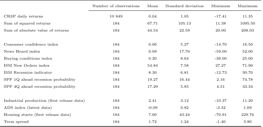
Table 1: Descriptive statistics: Q1 1970 - Q4 2015
Number of observations Mean Standard deviation Minimum Maximum
CRSP daily returns 10 849 0.04 1.05 -17.41 11.35 Sum of squared returns 184 67.71 105.13 11.38 1095.50 Sum of absolute value of returns 184 44.54 22.59 20.00 208.03
Consumer confidence index 184 0.06 5.27 -14.70 16.50
News Heard index 184 0.09 17.70 -59.00 52.00
Buying conditions index 184 0.20 8.64 -39.00 25.00 ISM New Orders index 184 54.84 7.58 27.27 71.90 ISM Recession indicator 184 8.30 6.81 -12.73 30.70 SPF 1Q ahead recession probability 184 19.27 16.44 2.16 74.78 SPF 4Q ahead recession probability 184 17.29 5.85 4.51 33.34
Industrial production (first release data) 184 2.41 3.12 -10.37 11.20 ADS index (latest data) 184 -0.09 0.82 -3.32 1.69 Housing starts (first release data) 184 7.00 43.24 -70.91 229.76
Term spread 184 1.72 1.24 -1.40 3.80
forward-looking variables, such as the four quarters ahead recession probability (0.07), and
the relatively high correlation with coincident or lagging indicators, such as the ADS index
(-0.45). The correlation between the recession probabilities one and four quarters ahead is
small (0.09), while for the other sentiment measures the sub-indices are highly correlated
with each other. Industrial production and the ADS index are highly correlated with the ISM
indices and the one quarter ahead recession probability, but only moderately correlated with
the consumer sentiment indicators, and not at all correlated with the four quarters ahead
recession probability. Housing starts is only moderately correlated with any of the sentiment
indicators, while the term spread has a relatively high correlation with the ISM Recession
indicator (0.46), but is only moderately correlated with the other sentiment measures. As
expected, the one quarter ahead recession probability is highly correlated with
contempo-raneous measures for economic activity, while the four quarters ahead probability is mostly
correlated with forward-looking variables, such as the term spread (-0.24).
As including many variables simultaneously in the MIDAS polynomial is infeasible, I use
principal components analysis to aggregate information in all macroeconomic and sentiment
variables. As the variables are measured on different scales I base the principal components
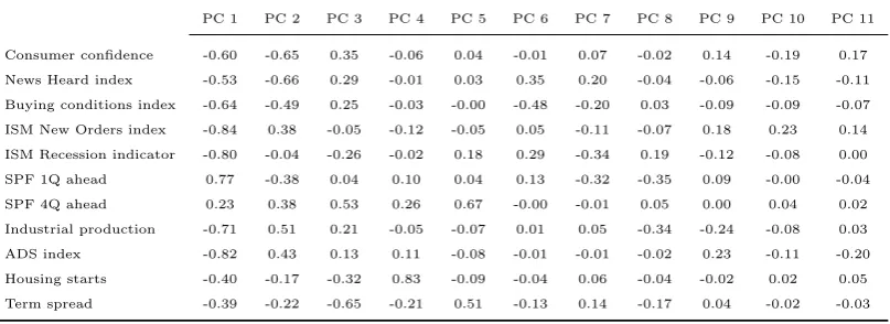
(PC) on the correlation matrix. Table 3 shows the correlations between the eleven principal
components and the eleven variables. The first PC is highly correlated with most of the
variables, but in particular with the ISM indices, the ADS index, industrial production and
the one quarter ahead recession probability. Hence it captures current business conditions. The
Table 2: Correlation matrix for the macro and sentiment variables
Σr2 Σ|r| CC NH BC NO RI IP HS ADS TS 1Q
Σ|r| 0.92 1 Consumer confidence -0.20 -0.20 1 News Heard index -0.19 -0.15 0.80 1 Buying conditions index -0.21 -0.21 0.74 0.55 1 ISM New Orders index -0.35 -0.40 0.24 0.19 0.33 1 ISM Recession Indicator -0.27 -0.27 0.39 0.40 0.40 0.66 1 Industrial production -0.22 -0.27 0.16 0.13 0.24 0.76 0.43 1 Housing starts -0.18 -0.17 0.20 0.22 0.25 0.19 0.34 0.11 1 ADS index -0.39 -0.45 0.27 0.18 0.33 0.83 0.56 0.78 0.30 1 Term spread 0.06 -0.01 0.19 0.17 0.22 0.26 0.46 0.05 0.21 0.09 1 SPF 1Q ahead 0.40 0.45 -0.20 -0.15 -0.30 -0.73 -0.53 -0.65 -0.19 -0.74 -0.24 1 SPF 4Q ahead 0.11 0.07 -0.19 -0.20 -0.20 -0.13 -0.21 -0.06 -0.16 0.01 -0.24 0.09
Σr2denotes the sum of squared returns,Σ|r|denotes the sum of absolute value of returns. Sample period: Q1 1970 - Q4 2015. First release data is used for industrial production and housing starts. Latest available data is used for the ADS index.
Table 3: Correlation between the principal components and the explanatory variables
PC 1 PC 2 PC 3 PC 4 PC 5 PC 6 PC 7 PC 8 PC 9 PC 10 PC 11
Consumer confidence -0.60 -0.65 0.35 -0.06 0.04 -0.01 0.07 -0.02 0.14 -0.19 0.17 News Heard index -0.53 -0.66 0.29 -0.01 0.03 0.35 0.20 -0.04 -0.06 -0.15 -0.11 Buying conditions index -0.64 -0.49 0.25 -0.03 -0.00 -0.48 -0.20 0.03 -0.09 -0.09 -0.07 ISM New Orders index -0.84 0.38 -0.05 -0.12 -0.05 0.05 -0.11 -0.07 0.18 0.23 0.14 ISM Recession indicator -0.80 -0.04 -0.26 -0.02 0.18 0.29 -0.34 0.19 -0.12 -0.08 0.00 SPF 1Q ahead 0.77 -0.38 0.04 0.10 0.04 0.13 -0.32 -0.35 0.09 -0.00 -0.04 SPF 4Q ahead 0.23 0.38 0.53 0.26 0.67 -0.00 -0.01 0.05 0.00 0.04 0.02 Industrial production -0.71 0.51 0.21 -0.05 -0.07 0.01 0.05 -0.34 -0.24 -0.08 0.03 ADS index -0.82 0.43 0.13 0.11 -0.08 -0.01 -0.01 -0.02 0.23 -0.11 -0.20 Housing starts -0.40 -0.17 -0.32 0.83 -0.09 -0.04 0.06 -0.04 -0.02 0.02 0.05 Term spread -0.39 -0.22 -0.65 -0.21 0.51 -0.13 0.14 -0.17 0.04 -0.02 -0.03
Sample period: Q1 1970 - Q4 2015. First release data is used for industrial production and housing starts. Latest
avail-able data is used for the ADS index.
second PC has the highest correlations with the consumer confidence indices. The third PC is
mostly correlated with the term spread and the four quarters ahead recession probability, but
also housing starts and the consumer confidence index. Thus it describes the forward-looking
components of the data. The remaining principal components are either primarily correlated
with just one variable or not very correlated with any of the variables. Hence, I use the first
three principal components as explanatory variables in the MIDAS polynomial.
5 In-sample results
In Section 5.1 I establish baseline results using the GARCH-MIDAS model with one
explana-tory variable.27
I largely confirm the results in Conrad and Loch (2014) using a different
27The estimations are executed in Matlab, building on the basic code provided by Engle et al. (2013).
[image:14.595.98.502.322.469.2]stock return index and real-time macroeconomic data. In Section 5.2 I include two different
explanatory variables in the same MIDAS polynomial in order to determine the relative and
combined importance of macroeconomic variables and survey-based sentiment data.
5.1 Baseline results
The optimal lag length (K) for the explanatory data in the long-term component is selected
based on the data. I choose the K which maximises the value of the log-likelihood function
when K is allowed to be 4, 8, 12, 16, 20 or 24 quarters. For all specifications the value of the
log-likelihood function is maximised at either 8 or 12 lags, levelling off after this. Therefore I
use three years of lagged data, i.e.,K = 12(quarterly data) for all models.28
I keep K fixed at 12 for the remainder of the paper.
Next, the shape of the weighting scheme (ϕk(ω1, ω2)), i.e., whether restricted (ω1 = 1)
before estimation or not, is determined for each explanatory variable based on a likelihood
ratio test (LRT) between the two specifications. As explained in Section 3, the restricted
scheme forces the weights to be decaying, i.e., recent data matters the most for long-term
volatility. In Table 4 I report the model preferred based on the LRT.29
The related p-value
is reported below the value of the LLF. The significance of the weight parameters in Table 4
relate to testingωi= 1.30
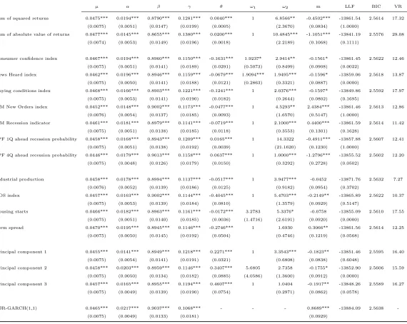
The GARCH mdoels parameters are consistently, robustly and similarly estimated for all
specifications (Table 4). The parameter determining the degree of asymmetry in volatility (γ) is always highly significant and positive, indicating, as expected, that lower-than-expected
returns lead to a higher conditional variance. Interestingly, the basic GJR-GARCH(1,1) model
has clearly the lowestγ. The choice of an asymmetric GARCH model is thus well-motivated.
α+β+γ/2 is clearly below one, indicating that the GARCH model is stationary. Overall, the GARCH parameters in the GARCH-MIDAS specifications get values roughly in line with
the estimates for the basic asymmetric GARCH(1,1) model (last row in Table 4).31
28Since by construction the last weight in the beta polynomial is zero, I useK+ 1lags in the estimation,
where the13th lag always gets the weight zero. This follows the convention in Conrad and Loch (2014).
29In the interest of parsimony significance levelα= 0.05is used. For the models driven by the four quarters
ahead recession probability, the term spread, and the third PC an unrestricted weighting scheme would have been chosen ifα= 0.10. Conrad and Loch (2014) used an unrestricted weighting scheme for the term spread.
30Testing
ωi= 0is of little interest, since zero is an arbitrary number in the context of the beta weighting scheme. Ifω1=ω2= 0the weighting scheme is symmetric and U-shaped.
31I do not report the estimates of the GARCH parameters for the rest of the paper. They are similarly and
robustly estimated throughout the specifications. Full results are available upon request.
Table 4: Estimation results for GARCH-MIDAS model with one explanatory variable
µ α β γ θ ω1 ω2 m LLF BIC VR
Sum of squared returns 0.0475*** 0.0194*** 0.8790*** 0.1281*** 0.0040*** 1 6.8566** -0.4502*** -13861.54 2.5614 17.32 (0.0075) (0.0051) (0.0147) (0.0199) (0.0005) (2.3670) (0.0834) (1.0000)
Sum of absolute value of returns 0.0477*** 0.0145*** 0.8655*** 0.1380*** 0.0200*** 1 10.4845*** -1.1051*** -13841.19 2.5576 29.08 (0.0074) (0.0053) (0.0149) (0.0196) (0.0018) (2.2189) (0.1068) (0.1111)
Consumer confidence index 0.0467*** 0.0194*** 0.8960*** 0.1150*** -0.1631*** 1.9237* 2.9414** -0.1561* -13861.45 2.5622 12.46 (0.0075) (0.0051) (0.0141) (0.0189) (0.0291) (0.5073) (0.8499) (0.0908) (0.0022)
News Heard index 0.0462*** 0.0196*** 0.8946*** 0.1159*** -0.0679*** 1.9094*** 1.9495*** -0.1596* -13859.06 2.5618 13.87 (0.0075) (0.0050) (0.0141) (0.0188) (0.0121) (0.2863) (0.3321) (0.0887) (0.0000)
Buying conditions index 0.0468*** 0.0166*** 0.8903*** 0.1221*** -0.1241*** 1 2.0376*** -0.1597* -13849.86 2.5592 17.97 (0.0075) (0.0053) (0.0141) (0.0190) (0.0182) (0.2644) (0.0802) (0.1695)
ISM New Orders index 0.0452*** 0.0148*** 0.9002*** 0.1173*** -0.0477*** 1 4.5293** 2.4384*** -13861.46 2.5613 12.86 (0.0076) (0.0054) (0.0137) (0.0185) (0.0093) (1.6570) (0.5147) (1.0000)
ISM Recession indicator 0.0461*** 0.0181*** 0.8979*** 0.1141*** -0.0719*** 1 2.1000*** 0.4400*** -13861.59 2.5614 11.42 (0.0075) (0.0051) (0.0138) (0.0185) (0.0118) (0.3553) (0.1301) (0.1628)
SPF 1Q ahead recession probability 0.0458*** 0.0168*** 0.8943*** 0.1209*** 0.0165*** 1 14.3322 -0.4911*** -13857.88 2.5607 12.41 (0.0075) (0.0051) (0.0138) (0.0192) (0.0039) (21.1620) (0.1230) (1.0000)
SPF 4Q ahead recession probability 0.0446*** 0.0179*** 0.9013*** 0.1158*** 0.0637*** 1 1.0000*** -1.2796*** -13855.52 2.5602 12.20 (0.0075) (0.0048) (0.0126) (0.0179) (0.0150) (0.3292) (0.2728) (0.0502)
Industrial production 0.0458*** 0.0178*** 0.8994*** 0.1137*** -0.0517*** 1 3.9477*** -0.0452 -13871.76 2.5632 7.27 (0.0076) (0.0052) (0.0139) (0.0186) (0.0125) (0.9182) (0.0954) (0.3702)
ADS index 0.0457*** 0.0163*** 0.9002*** 0.1144*** -0.4045*** 1 5.4703*** -0.2149** -13865.89 2.5622 10.37 (0.0075) (0.0053) (0.0139) (0.0184) (0.0810) (1.3579) (0.0929) (0.5147)
Housing starts 0.0466*** 0.0182*** 0.8963*** 0.1161*** -0.0172*** 3.2783 5.3376* -0.0758 -13855.09 2.5610 17.55 (0.0075) (0.0051) (0.0140) (0.0185) (0.0036) (1.4716) (2.6191) (0.0920) (0.0000)
Term spread 0.0470*** 0.0195*** 0.8945*** 0.1146*** -0.2746*** 1 1.6930 0.3066** -13861.56 2.5614 12.25 (0.0075) (0.0050) (0.0145) (0.0192) (0.0504) (0.4746) (0.1219) (0.0568)
Principal component 1 0.0455*** 0.0141*** 0.8949*** 0.1218*** 0.2271*** 1 3.3543*** -0.1823** -13851.46 2.5595 16.40 (0.0075) (0.0054) (0.0141) (0.0191) (0.0321) (0.6808) (0.0838) (0.6048)
Principal component 2 0.0458*** 0.0203*** 0.8959*** 0.1146*** 0.3407*** 5.6805 2.7358 -0.1755* -13852.90 2.5606 15.59 (0.0075) (0.0050) (0.0134) (0.0182) (0.0885) (4.0586) (1.3600) (0.0912) (0.0000)
Principal component 3 0.0457*** 0.0165*** 0.8955*** 0.1194*** 0.4607*** 1 1.0404 -0.1917** -13848.26 2.5589 16.27 (0.0075) (0.0049) (0.0139) (0.0190) (0.0754) (0.2971) (0.0862) (0.0578)
GJR-GARCH(1,1) 0.0465*** 0.0217*** 0.9037*** 0.1068*** - - - 0.8689*** -13884.09 2.5638 -(0.0075) (0.0049) (0.0133) (0.0181) (0.0929)
Bollerslev-Wooldridge QMLE robust standard errors are reported below the parameter estimates. *, ** and *** indicate significance at the 10%, 5% and 1% level,
respec-tively. LLF is the value of the log-likelihood function, BIC is the Bayesian Information Criteria and VR is the variance ratio from Section 3, multiplied by 100. The MIDAS
polynomial:log τt=m+θPKk=1ϕk(ω1, ω2)Xt−k, whereXstands for the explanatory data, as stated in the first column. All models are estimated with a restricted (ω1= 1)
and an unrestricted weighting scheme. The model reported in the table is chosen based on a likelihood ratio test between the restricted and unrestricted specifications. The
16
(a) Sum of squared returns (b) Sum of absolute value of
re-turns
(c) Consumer confidence index
(d) News Heard index (e) ISM New Orders index (f) ISM Recession indicator
(g) SPF 1Q ahead recession
prob-ability
(h) SPF 4Q ahead recession
prob-ability
(i) Industrial production
(j) Housing starts (k) ADS index (l) Term spread
[image:17.595.77.506.72.769.2](m) Principal component 1 (n) Principal component 2 (o) Principal component 3
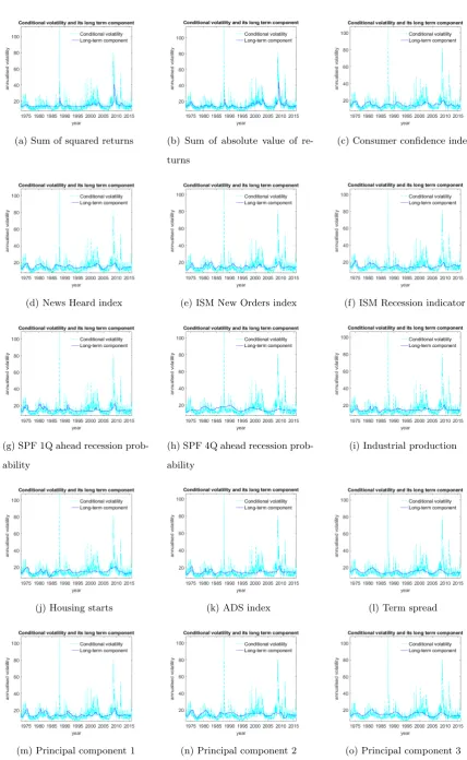
Figure 1 shows how the GARCH-MIDAS model decomposes volatility into two
compo-nents, by plotting total volatility and the extracted long-term component separately. It is
clear that the long-term components based on different variables capture long-term volatility
in very different ways. The parameter θ determines how the explanatory data affects long-term volatility. It is highly significant in all specifications and has the expected sign (Table 4):
positive for the realised volatility measures and the recession probabilities, and negative for
macroeconomic variables and consumer and business sentiment. A positive estimate for the
recession probabilities indicates that a higher probability of a recession among professional
forecasters translates into higher stock market volatility. The highly significant estimates for
the recession probabilities indicate that they can be useful in modelling long-term stock
mar-ket volatility. The estimates ofθfor all three principal components are positive, largely in line with the correlations between the factors and the explanatory variables (see Table 3). Overall
the results strongly support the countercyclical nature of long-term stock market volatility.
The variance ratio of the GARCH-MIDAS model where the long-term component is driven
by the quarterly sum of the lagged absolute value of returns is roughly 29%, which is clearly
greater than for any other variable, and clearly greater than for the model driven by the
quarterly sum of the lagged squared returns (17.3%). Realised volatility based on the absolute
value of returns thus seems to incorporate a large amount of useful information for explaining
long-term stock market volatility. The good in-sample fit is also evident from Figure 1b.
Considering the macroeconomic and sentiment data, the long-term components driven by
housing starts and the Buying conditions index explain a large share of the total variance
(more than 17%), while the long-term component based on the term spread explains 12.3%.
The principal components driven models have relatively high variance ratios of around 16%,
indicating it can be useful to summarise information. On the other hand, the variance of
the long-term component determined by industrial production only accounts for 7.3% of the
total variance. Based on the variance ratios, the forward-looking News Heard index and the
Buying conditions index outperform the main consumer confidence index.
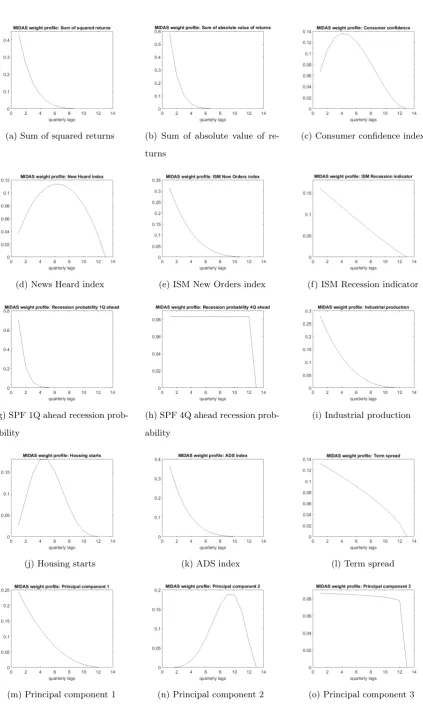
The weights of the twelve lags of the macroeconomic and confidence variables are
plot-ted in Figure 2. Engle et al. (2013) noplot-ted that ω1 = 1 is optimal for realised volatility, and
this is echoed in my results. Decaying weights is also intuitive: recent information in realised
volatility is more important than older information. For the consumer confidence indicators
18
(a) Sum of squared returns (b) Sum of absolute value of
re-turns
(c) Consumer confidence index
(d) News Heard index (e) ISM New Orders index (f) ISM Recession indicator
(g) SPF 1Q ahead recession
prob-ability
(h) SPF 4Q ahead recession
prob-ability
(i) Industrial production
(j) Housing starts (k) ADS index (l) Term spread
[image:19.595.85.509.65.780.2](m) Principal component 1 (n) Principal component 2 (o) Principal component 3
the optimal weighting schemes are often hump-shaped, indicating that older information is
more important for volatility than very recent information. Conrad and Loch (2014)
inter-preted hump-shaped weighting schemes as a sign that the variable is forward-looking, while
monotonously declining weights imply that the variable is lagging or coincidental.32
Thus,
business confidence, which gets decaying weights, seems to anticipate stock market
volatil-ity less than consumer confidence. The lags of the four quarters ahead recession probabilvolatil-ity
are equally weighted, while the fastest decay in weights is seen for the one quarter ahead
recession probability, for which only the first five lags get a non-zero weight. As expected,
industrial production and the ADS index have decaying weighting schemes, while the largest
weight for housing starts is on the fourth and fifth lags, which supports the perception that
housing starts is a forward-looking indicator. The first principal component has decaying
weights, the second one has a hump-shaped weighting scheme, while the third one has close
to equal weights for all lags. These weighting schemes seem plausible, as the first PC is mainly
correlated with indicators for current business conditions which have decaying weights
them-selves, the second one with consumer confidence data (hump-shaped weights), while the third
PC has the highest correlation with the term spread and the four quarters ahead recession
probability, which both have relatively flat weighting schemes.
These results remain robust to including realised volatility in the specifications (see
Ap-pendix 1), indicating that macroeconomic data and survey-based sentiment indicators explain
parts of the long-term stock market volatility not captured by past returns.33
.
5.2 Combining macroeconomic variables and sentiment indicators
In order to examine the combined and relative information content of macroeconomic
vari-ables and survey-based sentiment indicators I include one of both in the same MIDAS
poly-nomial (Table 5). The significance of their respective coefficients (θ1 and θ2) can be used to
assess whether both are simultaneously useful for explaining volatility. The variance ratios
re-veal whether the variables are able to explain more of the total conditional variance together
than on their own. As the term spread can also be interpreted as a sentiment indicator,
I include specifications where the term spread is combined with the other macroeconomic
32On the other hand, Asgharian et al. (2013) interpreted weights which are not monotonically decreasing
as counterintuitive, always enforcing the restrictionω1= 1.
33This is in line with the conclusion in, for example, Conrad and Loch (2014) and Asgharian et al. (2013)
data. As a robustness check, to control for the information in realised volatility, I also include
results with three explanatory variables in the MIDAS filter: the absolute value of returns
(RV), a macroeconomic variable and a sentiment indicator (Table 6).
For each variable I keep the earlier choice of a restricted or unrestricted weighting scheme,
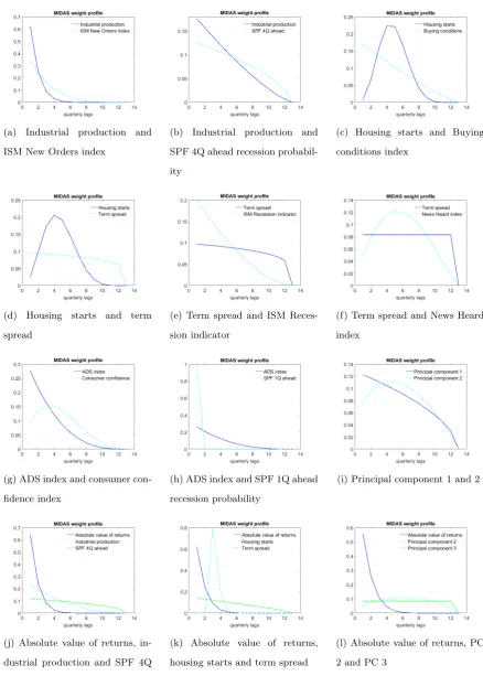
but re-estimate the weight parameter(s) (ωi). In most cases the weight parameter(s) are simi-lar regardless of the other variables included (compare, e.g., Table 4 with Table 5, and Table 10
with Table 6). For example, for the absolute value of returns and industrial production ω2
implies a very similar speed of decay in all specifications. For housing starts the inclusion
of RV occasionally leads to weighting schemes with almost all weight on the third lag (see
Figure 3k), but mostly it has a similar hump-shaped pattern as earlier. The term spread as
well as the four quarters ahead recession probability get in many cases very gradually
decay-ing weights. For the one quarter ahead recession probability all the weight is on the first lag
(ω2 ≈ 100in Table 5 and Table 6). This is not surprising as the information in the lags of
the recession probability can plausibly be assumed to be already included in other data.
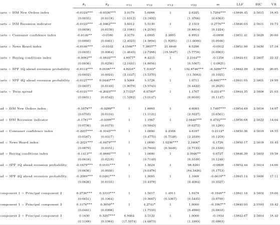
The intuitive sign ofθ is retained in all cases where the parameter is statistically signifi-cant. The effect of industrial production or the ADS index on long-term volatility is mostly
insignificant or only weakly significant when survey-based sentiment measures are included
(with the exception of the recession probabilities), while the sentiment indicators remain
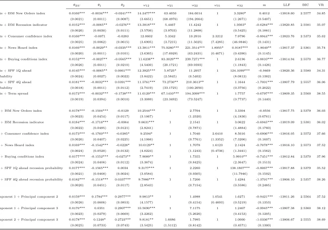
sig-nificant. This effect is clearly more pronounced when information in the absolute value of
returns is accounted for (Table 6). This implies sentiment indicators capture information in
and beyond backward-looking macroeconomic variables.
Housing starts get highly significant estimates forθ, and with the occasional exception of a consumer confidence indicator so do the sentiment indicators. Controlling for information
in absolute returns does not significantly influence these results. The term spread and the
sentiment indicators are simultaneously highly significant (Table 5), but when information in
the absolute value of returns is taken into account there is only weak evidence of sentiment
indicators containing additional useful information for long-term stock market volatility
(Ta-ble 6). It is noteworthy that the four quarter ahead recession probability is highly significant
throughout the specifications, indicating it includes information different from that in the
macroeconomic data and the absolute value of returns.
Table 5: Estimation results for GARCH-MIDAS model where macroeconomic data (θ1) and sentiment indicators (θ2) are combined
θ1 θ2 ω11 ω12 ω12 ω22 m LLF BIC VR
Industrial production + ISM New Orders index 0.0094 -0.0527*** 1 11.5561* 1 4.9374* 2.6929*** -13861.08 2.5630 12.85 (0.0150) (0.0128) (6.1113) (2.1013) (0.6852)
Industrial production + ISM Recession indicator -0.0297* -0.0569*** 1 2.3946** 1 2.4504*** 0.3794*** -13859.47 2.5627 12.64 (0.0160) (0.0134) (0.5426) (0.5120) (0.1299)
Industrial production + Consumer confidence index -0.0277 -0.1301*** 1 2.8377* 1.8151 3.2016* -0.0985 -13859.54 2.5636 14.07 (0.0201) (0.0366) (1.0516) (0.5636) (1.2498) (0.0950)
Industrial production + News Heard index -0.0307 -0.0607*** 1 1.9038 1.8017*** 2.0675** -0.0930 -13857.17 2.5631 15.46 (0.0248) (0.0145) (1.3685) (0.2928) (0.4777) (0.0974)
Industrial production + Buying conditions index -0.0144 -0.1087*** 1 3.2066* 1 2.1619*** -0.1309 -13849.78 2.5609 18.14 (0.0171) (0.0248) (1.1601) (0.3608) (0.0829)
Industrial production + SPF 1Q ahead recession probability -0.0305** 0.0125*** 1 2.7557*** 1 110.0872*** -0.3462*** -13855.28 2.5619 13.93 (0.0143) (0.0024) (0.6225) (18.4064) (0.1027)
Industrial production + SPF 4Q ahead recession probability -0.0659*** 0.0601*** 1 2.3224*** 1 1.6101 -1.0800*** -13843.98 2.5598 18.16 (0.0174) (0.0144) (0.5021) (0.6443) (0.2555)
Industrial production + Term spread -0.0334** -0.2182*** 1 3.9053** 1 1.9518 0.2787** -13856.40 2.5621 14.33 (0.0138) (0.0550) (1.1787) (0.8477) (0.1175)
ADS index + ISM New Orders index -0.0674 -0.0432*** 1 95.0806*** 1 3.8238** 2.1839*** -13860.57 2.5629 12.85 (0.0608) (0.0101) (18.8739) (1.3943) (0.5654)
ADS index + ISM Recession indicator -0.2155** -0.0499*** 1 3.7904*** 1 2.3083*** 0.2247 -13858.92 2.5626 12.91 (0.1085) (0.0148) (0.9516) (0.4976) (0.1598)
ADS index + Consumer confidence index -0.2492* -0.1088** 1 3.8644* 1.9296 3.6232 -0.1947** -13857.84 2.5632 14.92 (0.1405) (0.0424) (1.7069) (0.7273) (2.1272) (0.0914)
ADS index + News Heard index -0.2364* -0.0517*** 1 3.9626 1.8057** 1.9758** -0.1969** -13854.87 2.5627 16.14 (0.1282) (0.0170) (4.3496) (0.3477) (0.4516) (0.0889)
ADS index + Buying conditions index -0.1295 -0.1013*** 1 4.1363* 1 2.2044*** -0.1804** -13849.36 2.5608 18.18 (0.1175) (0.0263) (1.6389) (0.3635) (0.0848)
ADS index + SPF 1Q ahead recession probability -0.2185** 0.0114*** 1 3.6427*** 1 102.8511*** -0.4201*** -13855.14 2.5619 14.02 (0.1082) (0.0030) (1.0102) (27.5078) (0.0954)
ADS index + SPF 4Q ahead recession probability -0.4504*** 0.0568*** 1 3.2091** 1 1.5774 -1.2317*** -13840.93 2.5593 18.97 (0.1213) (0.0141) (0.8873) (0.7144) (0.2569)
ADS index + Term spread -0.2614*** -0.2010*** 1 5.4811*** 1 1.7930 0.1401 -13853.99 2.5617 15.06 (0.0921) (0.0566) (1.7233) (0.8110) (0.1347)
Table 5continued
θ1 θ2 ω11 ω12 ω12 ω22 m LLF BIC VR
Housing starts + ISM New Orders index -0.0124*** -0.0336*** 3.0179 5.6088 1 2.6225 1.7294*** -13848.45 2.5615 18.85 (0.0035) (0.0118) (1.6312) (3.1802) (1.3706) (0.6363)
Housing starts + ISM Recession indicator -0.0123*** -0.0462*** 3.6012 5.5130 1 2.1319 0.2776** -13846.03 2.5611 19.73 (0.0038) (0.0130) (2.1981) (4.2150) (0.8814) (0.1224)
Housing starts + Consumer confidence index -0.0146** -0.0580 3.3170 4.6905 2.3895 6.8953 -0.0898 -13851.41 2.5629 20.60 (0.0060) (0.0461) (2.4023) (4.3894) (1.9295) (11.6006) (0.0946)
Housing starts + News Heard index -0.0146*** -0.0102 4.1046** 7.3857** 21.6840 8.5296 -0.0912 -13851.90 2.5630 17.18 (0.0035) (0.0064) (1.4643) (2.7288) (19.5847) (5.7758) (0.0903)
Housing starts + Buying conditions index -0.0082** -0.0833*** 4.8977* 8.4215 1 2.2164** -0.1258 -13844.01 2.5607 22.32 (0.0036) (0.0236) (2.1431) (4.8056) (0.5367) ( 0.0825)
Housing starts + SPF 1Q ahead recession probability -0.0112*** 0.0108*** 4.9216* 7.3163* 1 132.8746*** -0.3298*** -13842.39 2.5604 20.65 (0.0032) (0.0024) (2.1447) (3.5370) (11.5682) (0.1025)
Housing starts + SPF 4Q ahead recession probability -0.0127*** 0.0440*** 3.5068 5.5728 1 1.0711 -0.8807*** -13841.05 2.5601 18.99 (0.0037) (0.0143) (1.9079) (3.5743) (0.4422) (0.2625)
Housing starts + Term spread -0.0121*** -0.2023*** 3.7123* 6.6700* 1 1.1767 0.2314** -13844.35 2.5608 21.03 (0.0031) (0.0542) (1.5282) (3.0147) (0.6030) (0.1147)
Term spread + ISM New Orders index -0.1678** -0.0299** 1 1.8883 1 4.6093 1.7497*** -13854.69 2.5618 14.97 (0.0703) (0.0134) (1.1121) (2.9227) (0.6561)
Term spread + ISM Recession indicator -0.1781** -0.0398** 1 1.1967 1 2.6646*** 0.4702*** -13856.68 2.5622 14.04 (0.0736) (0.0173) (0.5843) (0.6272) (0.1285)
Term spread + Consumer confidence index -0.2237*** -0.1043*** 1 1.0000 2.2166 4.6187 0.2112* -13850.36 2.5619 18.55 (0.0587) (0.0317) (0.4770) (0.7549) (2.2339) (0.1259)
Term spread + News Heard index -0.2021*** -0.0479*** 1 1.0000 1.9236*** 2.3406* 0.1720 -13850.17 2.5618 19.43 (0.0679) (0.0151) (0.7844) (0.3449) (0.7133) (0.1330)
Term spread + Buying conditions index -0.1413** -0.0886*** 1 1.0000 1 2.3946** 0.0727 -13846.39 2.5603 19.58 (0.0618) (0.0219) (0.7149) (0.5538) (0.1248)
Term spread + SPF 1Q ahead recession probability -0.1679*** 0.0101*** 1 1.3024 1 98.8281 -0.0809 -13852.44 2.5614 14.66 (0.0636) (0.0030) (0.6478) (84.3426) (0.1753)
Term spread + SPF 4Q ahead recession probability -0.2089*** 0.0481*** 1 1.3085 1 1.1668 -0.6619** -13845.14 2.5600 17.11 (0.0626) (0.0155) (0.4378) (0.4084) (0.3327)
Principal component 1 + Principal component 2 0.2736*** 0.3310*** 1 1.5617 1.4911 1.9478 -0.1948** -13841.16 2.5602 19.66 (0.0651) (0.1064) (0.3667) (0.5367) (0.5435) (0.0790)
Principal component 1 + Principal component 3 0.1178*** 0.3059** 1 4.2741* 1 1.0000 -0.1967** -13840.93 2.5593 19.42 (0.0441) (0.0998) (1.7533) (0.4990) (0.0810)
Principal component 2 + Principal component 3 0.1630 0.3207*** 6.9464 3.5122 1 1.0000 -0.1934 -13842.67 2.5604 18.42 (0.1188) (0.1084) (17.5974) (4.6873) (1.1889) (0.0863)
Bollerslev-Wooldridge QMLE robust standard errors are reported below the parameter estimates. *, ** and *** indicate significance at the 10%, 5% and 1% level, respectively.
LLF is the value of the log-likelihood function, BIC is the Bayesian Information Criteria and VR is the variance ratio from Section 3, multiplied by 100.
The MIDAS polynomial:log τt=m+θ1PKk=1ϕk(ω11, ω12)X1,t−k+θ2PKk=1ϕk(ω21, ω22)X2,t−k, whereX1denotes the macroeconomic data andX2 the sentiment data, as
Table 6: Estimation results for GARCH-MIDAS model where realised volatility (θRV), macroeconomic data (θ1) and sentiment indicator (θ2)
are combined
θRV θ1 θ2 ω12 ω21 ω22 ω31 ω32 m LLF BIC VR Industrial production + ISM New Orders index 0.0173*** 0.0142 -0.0329*** 10.4245*** 1 13.2304 1 6.9057 0.7831 -13827.76 2.5397 32.65
(0.0023) (0.0130) (0.0114) (3.5228) (9.2100) (3.7840) (0.6609)
Industrial production + ISM Recession indicator 0.0168*** -0.0057 -0.0355*** 11.3968*** 1 3.5415** 1 2.3334*** -0.6535*** -13829.37 2.5400 31.68 (0.0024) (0.0131) (0.0118) (3.4916) (1.0026) (0.4928) (0.1842)
Industrial production + Consumer confidence 0.0164*** -0.0109 -0.0678** 11.4497** 1 3.5776* 1.9565 4.5068 -0.9171*** -13830.03 2.5598 32.93 index (0.0025) (0.0153) (0.0332) (4.0824) (1.3792) (1.1862) (4.2416) (0.1494)
Industrial production + News Heard index 0.0164*** -0.0023 -0.0425*** 11.4362*** 1 4.7689 1.6088*** 1.7534*** -0.9388*** -13825.51 2.5590 34.19 (0.0024) (0.0124) (0.0117) (4.0009) (3.8697) (0.3135) (0.3740) (0.1438)
Industrial production + Buying conditions 0.0157*** -0.0010 -0.0661** 9.8321** 1 3.5994* 1 2.7471 -0.9094*** -13821.94 2.5386 35.02 index (0.0029) (0.0153) (0.0261) (4.3850) (1.3368) (1.2009) (0.1638)
Industrial production + SPF 1Q ahead 0.0159*** -0.0077 0.0079*** 10.5135** 1 3.7213*** 1 104.3401*** -1.0598*** -13828.21 2.5398 30.90 recession probability (0.0024) (0.0139) (0.0024) (4.1165) (1.0465) (11.0329) (0.1619)
Industrial production + SPF 4Q ahead 0.0167*** -0.0265* 0.0433*** 12.3181*** 1 3.1766** 1 1.4707 -1.6675*** -13813.58 2.5371 35.07 recession probability (0.0024) (0.0140) (0.0114) (3.3433) (1.0159) (0.5208) (0.2133)
Industrial production + Term spread 0.0180*** -0.0090 -0.1734*** 10.2906*** 1 4.9675* 1 2.3551 -0.7058*** -13818.66 2.5380 36.17 (0.0023) (0.0106) (0.0404) (3.2205) (2.0550) (0.8992) (0.1514)
ADS index + ISM New Orders index 0.0164*** -0.0317 -0.0237*** 12.2719*** 1 98.7464*** 1 4.5555 0.3461 -13828.83 2.5399 32.31 (0.0023) (0.0545) (0.0089) (3.5982) (20.7691) (2.4088) (0.5596)
ADS index + ISM Recession indicator 0.0170*** -0.0246 -0.0354*** 11.1753*** 1 93.7056*** 1 2.2089** -0.6791*** -13829.35 2.5400 31.64 (0.0022) (0.0506) (0.0120) (3.1818) (25.7094) (0.4798) (0.1815)
ADS index + Consumer confidence index 0.0161*** -0.0879 -0.0618* 11.7971** 1 5.3866 2.1214 4.9370 -0.9427*** -13829.78 2.5598 32.91 (0.0028) (0.1157) (0.0342) (4.4492) (3.3866) (1.2836) (4.6139) (0.1382)
ADS index + News Heard index 0.0160*** -0.0442 -0.0391*** 12.1426*** 1 122.6766*** 1.7173** 1.7936** -0.9311*** -13824.92 2.5589 34.14 (0.0023) (0.0564) (0.0114) (4.1862) (19.2362) (0.3600) (0.3859) (0.1249)
ADS index + Buying conditions index 0.0159*** 0.0196 -0.0704*** 9.5048* 1 17.5468 1 2.7237* -0.9185*** -13821.86 2.5386 35.12 (0.0031) (0.0685) (0.0224) (4.3807) (13.8407) (1.0141) (0.1599)
ADS index + SPF 1Q ahead recession probability 0.0161*** -0.0332 0.0079** 10.1930** 1 5.2771* 1 119.6018*** -1.0924*** -13828.42 2.5398 30.77 (0.0028) (0.1283) (0.0032) (4.6013) (2.2543) (14.5171) (0.1668)
ADS index + SPF 4Q ahead recession probability 0.0162*** -0.1856* 0.0427*** 12.8086*** 1 4.7718* 1 1.3853 -1.7159*** -13812.42 2.5369 35.28 (0.0026) (0.0992) (0.0112) (3.8418) (2.0861) (0.5004) (0.2008)
Table 6 continued
θRV θ1 θ2 ω12 ω21 ω22 ω31 ω32 m LLF BIC VR
Housing starts + ISM New Orders index 0.0160*** -0.0034*** -0.0241*** 14.2477*** 63.4650 184.6014 1 3.3280* 0.4012 -13818.60 2.5577 34.85 (0.0021) (0.0011) (0.0087) (3.6651) (68.4976) (194.2064) (1.2671) (0.5407)
Housing starts + ISM Recession indicator 0.0152*** -0.0065** -0.0276** 13.3818*** 5.4467 11.4242 1 1.9363* -0.6284*** -13820.85 2.5581 35.07 (0.0026) (0.0030) (0.0111) (3.5700) (3.9703) (11.2808) (0.5425) (0.1881)
Housing starts + Consumer confidence index 0.0160*** -0.0071 -0.0283 12.0602 5.3342 10.2916 2.3212 7.9796 -0.8944*** -13823.76 2.5373 35.62 (0.0025) (0.0062) (0.0615) (3.6905) (3.7215) (11.5025) (7.4285) (46.9846) (0.1431)
Housing starts + News Heard index 0.0160*** -0.0029** -0.0335*** 13.3811*** 75.9280*** 221.3514*** 1.8955* 0.9187*** 1.8649** -13817.37 2.5361 35.74 (0.0020) (0.0011) (0.0101) (3.6365) (17.6929) (63.2431) (0.4671) (0.4390) (0.1145)
Housing starts + Buying conditions index 0.0152*** -0.0027** -0.0565*** 11.6238** 83.3029*** 239.7271*** 1 2.6196 -0.8810*** -13814.94 2.5570 36.77 (0.0026) (0.0011) (0.0210) (4.5400) (20.1721) (69.9393) (1.1843) (0.1426)
Housing starts + SPF 1Q ahead 0.0145*** -0.0065** 0.0061*** 12.3925*** 5.8725* 11.2957 1 124.1099*** -0.9469 -13820.36 2.5580 34.31 recession probability (0.0024) (0.0027) (0.0022) (3.8422) (2.5845) (6.5402) (8.0812) (0.1382)
Housing starts + SPF 4Q ahead 0.0181*** -0.0032*** 0.0391*** 11.5761*** 73.2730** 210.3613** 1 1.1644 -1.7001*** -13807.79 2.5557 36.06 recession probability (0.0018) (0.0011) (0.0112) (2.7419) (33.1725) (100.2050) (0.3756) (0.2022)
Housing starts + Term spread 0.0172*** -0.0032*** -0.1738*** 11.6129*** 67.1410*** 194.3099*** 1 1.7757 -0.6797*** -13809.35 2.5560 38.55 (0.0019) (0.0394) (0.0010) (3.3089) (23.3492) (73.5247) (0.7737) (0.1440)
Term spread + ISM New Orders index 0.0178*** -0.1504*** -0.0129 10.2544*** 1 2.7704 1 3.3304 -0.0556 -13817.75 2.5379 36.03 (0.0023) (0.0454) (0.0117) (3.1067) (1.2320) (4.1836) (0.6761)
Term spread + ISM Recession indicator 0.0184*** -0.1716*** -0.0064 9.6631*** 1 2.1541 1 3.0622 -0.6945*** -13819.09 2.5381 36.02 (0.0022) (0.0485) (0.0121) (2.8241) (0.7871) (1.4884) (0.1760)
Term spread + Consumer confidence index 0.0173*** -0.1760*** -0.0385* 9.2594* 1 1.7040 2.6410 8.5016 -0.6906*** -13816.05 2.5572 37.66 (0.0026) (0.0407) (0.0225) (4.1066) (0.7761) (1.3352) (7.3206) (0.1607)
Term spread + News Heard index 0.0169*** -0.1542*** -0.0228* 10.0129** 1 1.7078 1.6123 2.1424 -0.7078*** -13816.10 2.5573 37.52 (0.0024) (0.0520) (0.0132) (4.0224) (1.1243) (0.4736) (1.3441) (0.1562)
Term spread + Buying conditions index 0.0177*** -0.1552*** -0.0273** 7.9089** 1 1.7355 1 5.9910** -0.7451*** -13812.84 2.5370 37.96 (0.0024) (0.0406) (0.0112) (3.3674) (0.8425) (2.3647) (0.1513)
Term spread + SPF 1Q ahead recession probability 0.0177*** -0.1565*** 0.0034 9.3177*** 1 2.2260 1 138.1807*** -0.8067*** -13817.88 2.5379 35.52 (0.0021) (0.0468) (0.0024) (3.0584) (0.9305) (11.7946) (0.1502)
Term spread + SPF 4Q ahead recession probability 0.0182*** -0.1518*** 0.0337*** 9.7986*** 1 1.7206 1 1.4284 -1.3701*** -13806.10 2.5357 38.26 (0.0020) (0.0451) (0.0117) (2.8543) (0.7154) (0.5586) (0.2485)
Principal component 1 + Principal component 2 0.0159*** 0.1784*** 0.2977*** 9.9813** 1 1.4988 1.0541 1.6271 -0.9421*** -13811.26 2.5564 37.52 (0.0026) (0.0606) (0.0853) (4.1577) (0.4154) (0.4693) (0.5219) (0.1353)
Principal component 1 + Principal component 3 0.0170*** 0.0351 0.2907*** 10.5690*** 1 7.1175 1 1.2407 -0.9945*** -13807.38 2.5360 38.12 (0.0023) (0.0279) (0.0669) (3.2262) (5.2626) (0.4153) (0.1205)
Principal component 2 + Principal component 3 0.0178*** 0.1248* 0.2723*** 9.8181** 1.6686 1.7995 1 1.0000 -1.0336*** -13806.67 2.5555 38.69 (0.0025) (0.0733) (0.0743) (3.5425) (1.5112) (0.8142) (0.4571) (0.1300)
Bollerslev-Wooldridge QMLE robust standard errors are reported below the parameter estimates. *, ** and *** indicate significance at the 10%, 5% and 1% level, respectively. LLF is the value of the
log-likelihood function, BIC is the Bayesian Information Criteria and VR is the variance ratio from Section 3, multiplied by 100.RVt=PNti=1|ri,t|.ω11= 1in all specifications.
The MIDAS polynomial:log τt=m+θRVPKk=1ϕk(1, ω12)RVt−k+θ1PKk=1ϕk(ω21, ω22)X1,t−k+θ2PKk=1ϕk(ω31, ω32)X2,t−k, whereX1denotes the macroeconomic data andX2the sentiment data, as
(a) Industrial production and
ISM New Orders index
(b) Industrial production and
SPF 4Q ahead recession
probabil-ity
(c) Housing starts and Buying
conditions index
(d) Housing starts and term
spread
(e) Term spread and ISM
Reces-sion indicator
(f) Term spread and News Heard
index
(g) ADS index and consumer
con-fidence index
(h) ADS index and SPF 1Q ahead
recession probability
(i) Principal component 1 and 2
(j) Absolute value of returns,
in-dustrial production and SPF 4Q
ahead recession probability
(k) Absolute value of returns,
housing starts and term spread
(l) Absolute value of returns, PC
[image:26.595.76.515.81.695.2]2 and PC 3
Figure 3: Weighting schemes of selected models from Table 5 and Table 6.
According to the variance ratios in Table 6 all specifications are able to explain more
than 30% of the total variation, some close to 40%, when the absolute value of returns is
included. However, comparing the variance ratios in Table 5 to those in Table 4 we can see
that the gains from including both macroeconomic and sentiment data into the same model
are in general relatively small, indicating that macroeconomic variables and sentiment data
contain mostly overlapping information for stock market volatility. On the other hand, for
example, the variance ratio for the model based on only the term spread is 12.3%, while the
variance ratio for the model with only the consumer confidence index is 12.5% (Table 4).
The long-term volatility component based on a combination of these series explains almost
19% of the total variance (Table 5). The model driven by only industrial production has a
variance ratio of 7.3%, while the model with the four quarter ahead recession probability has
a variance ratio of 12.2%. In the model combining these two series the variance ratio rises to
18.2%. The model combining housing starts with the term spread explain a significant 21%
of the total variance. The principal components summarise information in the economy well,
leading to some of the highest variance ratios (between 18.4% and 19.7%, Table 5).
6 Out-of-sample forecasts
The in-sample results highlighted the superiority of past absolute returns and forward-looking
data for stock return volatility. In this section I consider whether these results extend to an
out-of-sample context. I start by determining whether the baseline GARCH-MIDAS
mod-els (where the long-term component is based on one explanatory variable) outperform the
asymmetric GARCH(1,1) model in forecasting volatility. In order to narrow down the set
of potential forecasting models for stock return volatility I apply the Model Confidence Set
(MCS) procedure by Hansen et al. (2011) to the baseline models. The MCS approach
al-lows the construction of a set of models which contain the best model with a certain level of
confidence. In Section 6.2 I examine whether the models combining information from
macroe-conomic and sentiment data are superior to models with only one explanatory variable, from
an out-of-sample forecasting perspective.
As the short-term GARCH components are similar across all GARCH-MIDAS
specifica-tions, the largest gains in forecasting can be achieved in long-term forecasts. Thus, I consider
forecasts for 1, 2, 3 and 4 quarters ahead. The one-step ahead volatility prediction is given