Unanimous Prediction for 100% Precision with Application to
Learning Semantic Mappings
Fereshte Khani Stanford University [email protected]
Martin Rinard MIT
Percy Liang Stanford University [email protected]
Abstract
Can we train a system that, on any new input, either says “don’t know” or makes a prediction that is guaranteed to be cor-rect? We answer the question in the affir-mative provided our model family is well-specified. Specifically, we introduce the unanimity principle: only predict when all models consistent with the training data predict the same output. We operational-ize this principle for semantic parsing, the task of mapping utterances to logi-cal forms. We develop a simple, efficient method that reasons over the infinite set of all consistent models by only check-ing two of the models. We prove that our method obtains 100% precision even with a modest amount of training data from a possibly adversarial distribution. Empiri-cally, we demonstrate the effectiveness of our approach on the standard GeoQuery dataset.
1 Introduction
If a user asks a system “How many painkillers should I take?”, it is better for the system to say “don’t know” rather than making a costly incor-rect prediction. When the system is learned from data, uncertainty pervades, and we must manage this uncertainty properly to achieve our precision requirement. It is particularly challenging since training inputs might not be representative of test inputs due to limited data, covariate shift (Shi-modaira, 2000), or adversarial filtering (Nelson et al., 2009; Mei and Zhu, 2015). In this unforgiving setting, can we still train a system that is guaran-teed to either abstain or to make the correct pre-diction?
Our present work is motivated by the goal of
input output
area of Iowa area(IA)
cities in Ohio city(OH)
cities in Iowa city(IA)
mapping 1 mapping 2 mapping k
output 1 area(OH) area(OH)
output 2 area(OH) area(OH)
output k area(OH) OH
training examples
input
area of Ohio Ohio area
output area(Ohio)
don’t know
testing examples
unanimity
... ...
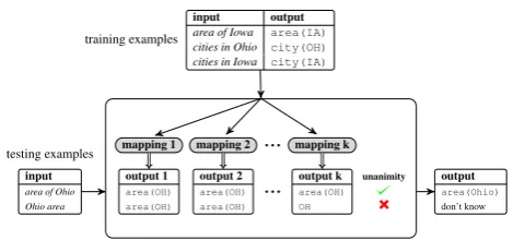
Figure 1: Given a set of training examples, we computeC, the set of all mappings consistent with the training examples. On an inputx, if all map-pings in C unanimously predict the same output, we return that output; else we return “don’t know”.
building reliable question answering systems and natural language interfaces. Our goal is to learn a semantic mapping from examples of utterance-logical form pairs (Figure 1). More generally, we assume the input x is a bag (multiset) of source atoms (e.g., words{area,of,Ohio}), and the out-put y is a bag of target atoms (e.g., predicates
{area,OH}). We consider learning mappingsM
that decompose according to the multiset sum:
M(x) = ]s∈xM(s) (e.g.,M({Ohio}) = {OH}, M({area,of,Ohio}) = {area,OH}). The main challenge is that an individual training example (x, y)does not tell us which source atoms map to which target atoms.1
How can a system be 100% sure about some-thing if it has seen only a small number of pos-sibly non-representative examples? Our approach is based on what we call theunanimity principle (Section 2.1). LetMbe a model family that con-tains the true mapping from inputs to outputs. Let
C be the subset of mappings that are consistent
1A semantic parser further requires modeling the context
dependence of words and the logical form structure joining the predicates. Our framework handles these cases with a different choice of source and target atoms (see Section 4.2).
[image:1.595.308.543.218.328.2]with the training data. If all mappings M ∈ C
unanimously predict the same output on a test in-put, then we return that output; else we return “don’t know” (see Figure 1). The unanimity prin-ciple provides robustness to the particular input distribution, so that we can tolerate even adver-saries (Mei and Zhu, 2015), provided the training outputs are still mostly correct.
To operationalize the unanimity principle, we need to be able to efficiently reason about the pre-dictions of all consistent mappingsC. To this end, we represent a mapping as a matrixM, whereMst
is number of times target atomt(e.g.,OH) shows up for each occurrence of the source atoms(e.g., Ohio) in the input. We show that unanimous pre-diction can be performed by solving two integer linear programs. With a linear programming re-laxation (Section 3), we further show that check-ing unanimity overCcan be done very efficiently without any optimization but rather by check-ing the predictions of just two random mappcheck-ings, while still guaranteeing 100% precision with prob-ability1(Section 3.2).
We further relax the linear program to a linear system, which gives us a geometric view of the unanimity: We predict on a new input if it can be expressed as a “linear combination” of the training inputs. As an example, suppose we are given train-ing data consisttrain-ing of (CI) cities in Iowa, (CO) cities in Ohio, and (AI) area of Iowa (Figure 1). We can compute (AO) area of Ohio by analogy: (AO) = (CO) - (CI) + (AI). Other reasoning pat-terns fall out from more complex linear combina-tions.
We can handle noisy data (Section 3.4) by ask-ing for unanimity over additional slack variables. We also show how the linear algebraic formulation enables other extensions such as learning from denotations (Section 5.1), active learning (Sec-tion 5.2), and paraphrasing (Sec(Sec-tion 5.3). We vali-date our methods in Section 4. On artificial data generated from an adversarial distribution with noise, we show that unanimous prediction obtains 100% precision, whereas point estimates fail. On GeoQuery (Zelle and Mooney, 1996), a standard semantic parsing dataset, where our model as-sumptions are violated, we still obtain 100% pre-cision. We were able to reach 70% recall on recov-ering predicates and 59% on full logical forms.
source atoms target atoms {area,of,Iowa} {area,IA} {cities,in,Ohio} {city,OH} {cities,in,Iowa} {city,IA}
mapping 1
cities→ {city}
in → {}
of → {}
area → {area} Iowa→ {IA} Ohio→ {OH}
mapping 2
cities→ {} in → {city}
of → {}
area → {area} Iowa→ {IA} Ohio→ {OH}
mapping 3
cities→ {city}
in → {}
of → {area} area → {} Iowa→ {IA} Ohio→ {OH}
mapping 4
[image:2.595.307.541.64.178.2]cities→ {} in → {city} of → {area} area → {} Iowa→ {IA} Ohio→ {OH}
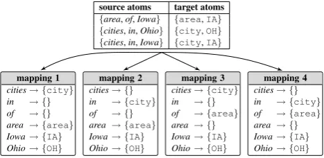
Figure 2: Given the training examples in the top table, there are exactly four mappings consistent with these training examples.
2 Setup
We represent an input x(e.g., area of Ohio) as a bag (multiset) of source atoms and an output y
(e.g., area(OH)) as a bag of target atoms. In the simplest case,source atomsare words and tar-get atomsare predicates—see Figure 2(top) for an example.2 We assume there is a true mapping M∗ from a source atom s (e.g., Ohio) to a bag
of target atoms t = M∗(s) (e.g., {OH}). Note
thatM∗ can also map a source atomsto no
tar-get atoms (M∗(of) ={}) or multiple target atoms
(M∗(grandparent) = {parent,parent}). We
extend M∗ to bag of source atoms via multiset
sum:M∗(x) =]
s∈xM∗(s).
Of course, we do not know M∗ and must
estimate it from training data. Our train-ing examples are input-output pairs D =
{(x1, y1), . . . ,(xn, yn)}. For now, we assume that
there is no noise so thatyi =M∗(xi); Section 3.4
shows how to deal with noise. Our goal is to out-put amappingMˆ that maps each inputxto either a bag of target atoms or “don’t know.” We say that Mˆ has 100% precision if Mˆ(x) = M∗(x)
whenever Mˆ(x) is not “don’t know.” The chief difficulty is that the source atomsxi and the
tar-get atomsyiare unaligned. While we could try to
infer the alignment, we will show that it is unnec-essary for obtaining 100% precision.
2.1 Unanimity principle
LetMbe the set of mappings (which contains the true mapping M∗). Let C be the subset of
map-2Our semantic parsing experiments (Section 4.2) use
S=
ar
ea
of Ohio cities in Iowa
" #
area of Iowa 1 1 0 0 0 1
cities in Ohio 0 0 1 1 1 0
cities in Iowa 0 0 0 1 1 1
M =
area city OH IA
area 1 0 0 0
of 0 0 0 0
Ohio 0 0 1 0
cities 0 1 0 0
in 0 0 0 0
Iowa 0 0 0 1
T =
area city OH IA
" #
[image:3.595.97.500.64.150.2]area(IA) 1 0 0 1 city(OH) 0 1 1 0 city(IA) 0 1 0 1
Figure 3: Our training data encodes a system of linear equationsSM = T, where the rows ofS are inputs, the rows ofT are the corresponding outputs, andM specifies the mapping between source and target atoms.
pings consistent with the training examples.
Cdef= {M ∈ M |M(xi) =yi,∀i= 1, . . . , n}
(1) Figure 2 shows the four mappings consistent with the training set in our running example. LetF be the set ofsafe inputs, those on which all mappings inCagree:
F def= {x:|{M(x) :M ∈ C}|= 1}. (2)
Theunanimity principledefines a mappingMˆ that returns the unanimous output on F and “don’t know” on its complement. This choice obtains the following strong guarantee:
Proposition 1. For each safe input x ∈ F, we
haveMˆ(x) =M∗(x). In other words,M obtains
100% precision.
Furthermore,Mˆ obtains the best possible recall given this model family subject to 100% precision, since for anyx6∈ F there are at least two possible outputs generated by consistent mappings, so we cannot safely guess one of them.
3 Linear algebraic formulation
To solve the learning problem laid out in the previ-ous section, let us recast the problem in linear al-gebraic terms. Letns(nt) be the number of source
(target) atom types. First, we can represent the bag x (y) as a ns-dimensional (nt-dimensional)
row vector of counts; for example, the vector
form of “area of Ohio” is ar
ea
of Ohio cities in Iowa
[1 1 1 0 0 0].
We represent the mapping M as a non-negative integer-valued matrix, whereMstis the number of
times target atomtappears in the bag that source atomsmaps to (Figure 3). We also encode then
training examples as matrices:Sis ann×ns
ma-trix where thei-th row isxi;Tas ann×ntmatrix
where thei-th row isyi. Given these matrices, we
can rewrite the set of consistent mappings (2) as:
C ={M ∈Zns×nt
≥0 :SM =T}. (3)
See Figure 3 for the matrix formulation ofS and
T, along with one possible consistent mappingM
for our running example.
3.1 Integer linear programming
Finding an element ofC as defined in (3) corre-sponds to solving an integer linear program (ILP), which is NP-hard in the worst case, though there exist relatively effective off-the-shelf solvers such as Gurobi. However, onesolution is not enough. To check whether an input x is in the safe set
F (2), we need to check whether all mappings
M ∈ Cpredict the same output onx; that is,xM
is the same for allM ∈ C.
Our insight is that we can check whetherx∈ F
by solving just two ILPs. Recall that we want to know if the output vectorxM can be different for differentM ∈ C. To do this, we pick a random vectorv∈Rnt, and consider the scalar projection
xMv. The first ILP maximizes this scalar and the second one minimizes it. If both ILPs return the same value, then with probability 1, we can con-clude thatxM is the same for all mappingsM ∈ C
and thus x ∈ F. The following proposition for-malizes this:
Proposition 2. Let x be any input. Let v ∼
N(0, Int×nt) be a random vector. Let a =
minM∈CxMv and b = maxM∈CxMv. With
probability 1,a=biffx∈ F.
Proof. Ifx ∈ F, there is only one outputxM, so
a = b. If x 6∈ F, there exists two M1, M2 ∈ C
(6,0,0) (0,6,0)
(0,0,0) p1
p2
R
P
a 2-dimensional ball
z≤0
−z≤0
−x≤0
−y≤0
[image:4.595.114.247.64.178.2]x+y≤6
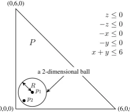
Figure 4: Our goal is to find two points p1, p2 in
the relative interior of a polytopePdefined by in-equalities shown on the right. The inin-equalitiesz≤
0and−z ≤0are always active. Therefore, P is a2-dimensional polytope. One solution to the LP (6) isα∗ = 1, p∗ = (1,1,0), ξ∗> = [0,0,1,1,1],
which results in p1 = (1,1,0)with R = 1/√2.
The other point p2 is chosen randomly from the
ball of radiusR.
M2)∈R1×ntis nonzero. The probability ofwv =
0 is zero because the space orthogonal tow is a (nt−1)-dimensional space whilevis drawn from a nt-dimensional space. Therefore, with probability
1, xM1v 6= xM2v. Without loss of generality, a≤xM1v < xM2v ≤b, soa6=b.
3.2 Linear programming
Proposition 2 requires solving two non-trivial ILPs per inputat test time. A natural step is to relax the integer constraint so that we solve two LPs instead.
CLPdef= {M ∈R≥ns0×nt |SM =T} (4) FLPdef= {x:|{M(x) :M ∈ CLP}|= 1}. (5)
The set of consistent mappings is larger (CLP ⊇ C), so the set of safe inputs is smaller (FLP ⊆ F). Therefore, if we predict only on FLP, we
still maintain 100% precision, although the recall could be lower.
Now we will show how to exploit the convex-ity of CLP (unlikeC) to avoid solving any LPs at
test time at all. The basic idea is that if we choose two mappingsM1, M2∈ CLP“randomly enough”,
whetherxM1 = xM2 is equivalent to unanimity
over CLP. We could try to sample M1, M2
uni-formly from CLP, but this is costly. We instead
show that “less random” choice suffices. This is formalized as follows:
Proposition 3. LetXbe a finite set of test inputs.
Letdbe the dimension ofCLP. LetM1be any
map-ping in CLP, and let vec(M2) be sampled from a
proper density over ad-dimensional ball lying in
CLP centered at vec(M1). Then, with probability
1, for allx∈X,xM1 =xM2impliesx∈ FLP.
Proof. We will prove the contrapositive. If x 6∈ FLP, then xM is not the same for all M ∈ CLP. Without loss of generality, assume not all M ∈ CLP agree on the i-th component of xM.
Note that (xM)i = tr(Meix), which is the
inner product of vec(M) and vec(eix). Since
(xM)i is not the same for all M ∈ CLP andCLP
is convex, the projection of CLP onto vec(eix)
must be a one-dimensional polytope. For both vec(M1) and vec(M2) to have the same
projec-tion on vec(eix), they would have to both lie
in a (d−1)-dimensional polytope orthogonal to vec(eix). Since vec(M2)is sampled from a proper
density over ad-dimensional ball, this has proba-bility0.
Algorithm. We now provide an algorithm to
find two points p1, p2 inside a general d
-dimensional polytopeP ={p :Ap≤b} satisfy-ing the conditions of Proposition 3, where for clar-ity we have simplified the notation from vec(Mi)
topiandCLPtoP.
We first find a pointp1in the relative interior of P, which consists of points for which the fewest number of inequalitiesjare active (i.e.,ajp=bj).
We can achieve this by solving the following LP from Freund et al. (1985):
max1>ξs.t. Ap+ξ ≤αb,0≤ξ≤1, α≥1.
(6)
Here,ξj is a lower bound on the slack of
inequal-ityj, andα scales up the polytope so that all the
ξj that can be positive are exactly 1 in the
opti-mum solution. Importantly, ifξj = 0, constraint j is always active for all solutions p ∈ P. Let (p∗, ξ∗, α∗)be an optimal solution to the LP. Then
defineA1as the submatrix ofAcontaining rowsj
for whichξ∗
j = 1, andA0consist of the remaining
rows for whichξ∗ j = 0.
The above LP gives us p1 = p∗/α∗, which
lies in the relative interior of P (see Fig-ure 4). To obtain p2, define a radius R def=
(αmaxj:ξ∗
j=1kajk2)−1. Let the columns of
ma-trixN form an orthonormal basis of the null space ofA0. Samplev from a unitd-dimensional ball
centered at0, and setp2 =p1+RNv.
To show that p2 ∈ P: First, p2 satisfies the
always-active constraintsj,a>
Algorithm 1Our linear programming approach.
procedureTRAIN
Input:Training examples
Output:Generic mappings(M1, M2)
DefineCLPas explained in (4).
ComputeM1and a radiusRby solving an LP (6). SampleM2from a ball with radiusRaroundM1. return(M1, M2)
end procedure
procedureTEST
Input:inputx, mappings(M1, M2)
Output:A guaranteed correctyor “don’t know”
Computey1=xM1andy2=xM2.
ify1=y2then returny1
else return“don’t know”
end if end procedure
by definition of null space. For non-activej, the LP ensures thata>
j p1+α−1 ≤bj, which implies a>
j(p1+RNv)≤bj.
Algorithm 1 summarizes our overall procedure: At training time, we solve a single LP (6) and draw a random vector to obtain M1, M2
satisfy-ing Proposition 3. At test time, we simply apply
M1 andM2, which scales only linearly with the
number of source atoms in the input.
3.3 Linear system
To obtain additional intuition about the unanimity principle, let us relax CLP (4) further by
remov-ing the non-negativity constraint, which results in a linear system. Define the relaxed set of consis-tent mappings to be all the solutions to the linear system and the relaxed safe set accordingly:
CLSdef= {M ∈Rns×nt |SM =T} (7) FLSdef= {x:|{M(x) :M ∈ CLS}|= 1}. (8)
Note that CLS is an affine subspace, so each M ∈ CLS can be expressed asM0 +BA, where M0is an arbitrary solution,Bis a basis for the null
space ofSandAis an arbitrary matrix. Figure 5 presents the linear system for four training exam-ples. In the rare case thatS has full column rank (if we have many training examples), then the left inverse ofSexists, and there is exactly one consis-tent mapping, the true one (M∗ = S†T), but we
do not require this.
Let’s try to explore the linear algebraic structure in the problem. Intuitively, if we know area of Ohiomaps to area(OH)andOhiomaps to OH, then we should concludearea of maps toareaby subtracting the second example from the first. The following proposition formalizes and generalizes this intuition by characterizing the relaxed safe set:
Proposition 4. The vectorxis in row space ofS
iffx∈ FLS.
S
z }| {
ar
ea
of Ohio cities in Iowa
" #
area of Iowa 1 1 0 0 0 1 +1 cities in Ohio 0 0 1 1 1 0 +1 cities in Iowa 0 0 0 1 1 1 −1
[ ]
area of Ohio 1 1 1 0 0 0
T
z }| {
area city OH IA
" #
area(IA) 1 0 0 1 +1
city(OH) 0 1 1 0 +1
city(IA) 0 1 0 1 −1
[ ]
area(OH) 1 0 1 0
Figure 6: Under the linear system relaxation, we can predict the target atoms for the new inputarea of Ohioby adding and subtracting training exam-ples (rows ofSandT).
Proof. Ifxis in the row space ofS, we can writex
as a linear combination ofSfor some coefficients
α ∈ Rn: x = α>S. Then for allM ∈ C LS, we
haveSM =T, soxM =α>SM =α>T, which
is the unique output3 (See Figure 6). Ifx ∈ FLS
is safe, then there exists aysuch that for allM ∈ CLS,xM =y. Recall that each element ofCLScan
be decomposed intoM0+BA. Forx(M0+BA)
to be the same for eachA,xshould be orthogonal to each column ofB, a basis for the null space of
S. This means thatxis in the row space ofS.
Intuitively, this proposition says that stitching new inputs together by adding and subtracting ex-isting training examples (rows ofS) gives you ex-actly the relaxed safe setFLS.
Note that relaxations increases the set of con-sistent mappings (CLS ⊇ CLP ⊇ C), which has
the contravariant effect of shrinking the safe set (FLS ⊆ FLP ⊆ F). Therefore, using the
relax-ation (predicting when x ∈ FLS) still preserves
100% precision.
3.4 Handling noise
So far, we have assumed that our training exam-ples are noiseless, so that we can directly add the
3There might be more than one set of coefficients (α
1, α2)
for writingx. However, they result to a same output:α>
1S=
α>
S
z }| {
area of Ohio cities in Iowa
1 1 0 0 0 1
0 0 1 1 1 0
0 0 0 1 1 1
1 1 1 1 1 0
×M=
T
z }| {
area city OH IA
1 0 0 1
0 1 1 0
0 1 0 1
1 1 1 0
=⇒ M=
M0
z }| {
area city OH IA
area 1 0 0 0 of 0 0 0 0 Ohio 0 0 1 0 cities 0 1 0 0 in 0 0 0 0 Iowa 0 0 0 1
+ B
z }| {
−1 0
1 0
0 0
0 −1
0 1 0 0 × A
z }| {
a1,1 a1,2 a1,3 a1,4
a2,1 a2,2 a2,3 a2,4
[image:6.595.79.515.65.135.2]
Figure 5: Under the linear system relaxation, all solutionsM toSM = T can be expressed asM =
M0+BA, whereB is the basis for the null space ofS andAis arbitrary. RowssofBwhich are zero
(OhioandIowa) correspond to the safe source atoms (though not the only safe inputs).
constraintSM = T. Now assume that an adver-sary has made at most nmistakes additions to and
deletions of target atoms across the examples in
T, but of course we do not know which examples have been tainted. Can we still guarantee 100% precision?
The answer is yes for the ILP formulation: we simply replace the exact match condition (SM =
T) with a weaker one:kSM−Tk1≤nmistakes(*).
The result is still an ILP, so the techniques from Section 3.1 readily apply. Note that as nmistakes
increases, the set of candidate mappings grows, which means that the safe set shrinks.
Unfortunately, this procedure is degenerate for linear programs. If the constraint (*) is not tight, thenM+Ealso satisfies the constraint for any ma-trixEof small enough norm. This means that the consistent mappingsCLP will be full-dimensional
and certainly not be unanimous on any input. Another strategy is to remove examples from the dataset if they could be potentially noisy. For each training examplei, we run the ILP (*) on all but the i-th example. If the i-th example is not in the resulting safe set (2), we remove it. This procedure produces a noiseless dataset, on which we can apply the noiseless linear program or linear system from the previous sections.
4 Experiments
4.1 Artificial data
We generated a true mappingM∗from 50 source
atoms to 20 target atoms so that each source atom maps to 0–2 target atoms. We then created 120 training examples and 50 test examples, where the length of every input is between 5 and 10. The source atoms are divided into 10 clusters, and each input only contains source atoms from one cluster. Figure 7a shows the results for F (integer lin-ear programming),FLP(linear programming), and
FLS(linear system). All methods attain 100%
pre-cision, and as expected, relaxations lead to lower recall, though they all can reach 100% recall given enough data.
Comparison with point estimation. Recall that
the unanimity principle Mˆ reasons over the en-tire set of consistent mappings, which allows us to be robust to changes in the input distribution, e.g., from training set attacks (Mei and Zhu, 2015). As an alternative, consider computing the point esti-mateMpthat minimizeskSM−Tk22(the solution
is given byMp = S†T). The point estimate, by
minimizing the average loss, implicitly assumes i.i.d. examples. To generate output for inputxwe computey = xMp and round each coordinateyt
to the closest integer. To obtain a precision-recall tradeoff, we set a thresholdand if for all target atomst, the interval[yt−, yt+)contains an
in-teger, we setytto that integer; otherwise we report
“don’t know” for inputx.
To compare unanimous predictionMˆ and point estimation Mp, for each f ∈ {0.2,0.5,0.7}, we
randomly generate 100 subsampled datasets con-sisting of an f fraction of the training examples. For Mp, we sweep across {0.0,0.1, . . . ,0.5}
to obtain a ROC curve. In Figure 7c(left/right), we select the distribution that results in the max-imum/minimum difference between F1( ˆM) and F1(Mp) respectively. As shown, Mˆ has always
100% precision, while Mp can obtain less 100%
precision over its full ROC curve. An adversary can only hurt the recall of unanimous prediction.
Noise. As stated in Section 3.4, our algorithm
has the ability to guarantee 100% precision even when the adversary can modify the outputs. As we increase the number of predicate addi-tions/deletions (nmistakes), Figure 7b shows that
0 0.2 0.4 0.6 0.8 1 0
0.2 0.4 0.6 0.8 1
Fraction of training data
Recall
precision (all) recall (ILP) recall (LP) recall (LS)
(a) All the relaxations reach 100% recall; relaxation re-sults in slightly slower con-vergence.
0 30 60 90 120 150 0
0.2 0.4 0.6 0.8 1
nmistakes precision (ILP) recall (ILP)
(b) Size of the safe set shrinks with increasing number of mistakes in the training data.
0 0.2 0.4 0.6 0.8 1 0.4
0.6 0.8 1
Recall
Pr
ecision
Mp(0.2) Mˆ(0.2) Mp(0.5) Mˆ(0.5) Mp(0.7) Mˆ(0.7)
0 0.2 0.4 0.6 0.8 1 0.4
0.6 0.8 1
Recall
Pr
ecision
Mp(0.2) Mˆ(0.2) Mp(0.5) Mˆ(0.5) Mp(0.7) Mˆ(0.7)
[image:7.595.87.506.60.196.2](c) Performance of the point estimate (Mp) and unani-mous prediction (Mˆ) when the inputs are chosen adver-sarially forMp(left) and forMˆ (right).
Figure 7: Our algorithm always obtains 100% precision with (a) different amounts of training examples and different relaxations, (b) existence of noise, and (c) adversarial input distributions.
0 0.2 0.4 0.6 0.8 1 0
0.2 0.4 0.6 0.8 1
Percentage of data
Recall
precision (LS) recall (LS)
Figure 8: We maintain 100% precision while re-call increases with the number of training exam-ples.
the training outputs.
4.2 Semantic parsing on GeoQuery
We now evaluate our approach on the standard GeoQuery dataset (Zelle and Mooney, 1996), which contains 880 utterances and their corre-sponding logical forms. The utterances are ques-tions related to the US geography, such as: “what river runs through the most states”. We use the standard 600/280 train/test split (Zettlemoyer and Collins, 2005). After replacing entity names by their types4 based on the standard entity lexicon,
there are 172 different words and 57 different predicates in this dataset.
Handling context. Some words are polysemous
in that they map to two predicates: in “largest river” and “largest city”, the word largest maps
tolongestandbiggest, respectively.
There-fore, instead of using words as source atoms, we
4If an entity name has more than one type we replace it
by concatenating all of its possible types.
use bigrams, so that each source atom always maps to the same target atoms.
Reconstructing the logical form. We define
target atoms to include more information than just the predicates, which enables us to reconstruct logical forms from the predicates. We use the variable-free functional logical forms (Kate et al., 2005), in which each target atom is a predicate conjoined with its argument order (e.g.,loc 1or
loc 2). Table 1 shows two different choices of
target atoms. At test time, we search over all possi-ble “compatipossi-ble” ways of combining target atoms into logical forms. If there is exactly one, then we return that logical form and abstain otherwise. We call a predicate combination “compatible” if it ap-pears in the training set.
We put a “null” word at the end of each sen-tence, and collapsed the loc and traverse
predicates. To deal with noise, we minimized
kSM −Tk1 over real-valued mappings and
re-moved any example (row) with non-zero residual. We perform all experiments using the linear sys-tem relaxation. Training takes under 30 seconds.
Figure 8 shows precision and recall as a func-tion of the number of the training examples. We obtain 70% recall over predicates on the test ex-amples. 84% of these have a unique compatible way of combining target atoms into a logical form, which results in a 59% recall on logical forms.
[image:7.595.99.266.250.386.2]ut-utterances logical form (A) target atoms (A) logical form (B) target atoms (B) cities traversed by the Columbia city(x),loc(x,Columbia) city,loc,Columbia city(loc 1(Columbia)) city,loc 1,Columbia
[image:8.595.339.494.170.292.2]cities of Texas city(x),loc(Texas,x) city,loc,Texas city(loc 2(Texas)) city,loc 2,Texas
Table 1: Two different choices of target atoms: (A) shows predicates and (B) shows predicates conjoined with their argument position. (A) is sufficient for simply recovering the predicates, whereas (B) allows for logical form reconstruction.
terance contains a proper noun. With negative mappings,nullmaps toall:e, while each proper noun maps to its proper predicateminusall:e.
There is a lot of work in semantic parsing that tackles the GeoQuery dataset (Zelle and Mooney, 1996; Zettlemoyer and Collins, 2005; Wong and Mooney, 2007; Kwiatkowski et al., 2010; Liang et al., 2011), and the state-of-the-art is 91.1% pre-cision and recall (Liang et al., 2011). However, none of these methods can guarantee 100% pre-cision, and they perform more feature engineer-ing, so these numbers are not quite comparable. In practice, one could use our unanimous prediction approach in conjunction with others: For example, one could run a classic semantic parser and simply certify 59% of the examples to be correct with our approach. In critical applications, one could use our approach as a first-pass filter, and fall back to humans for the abstentions.
5 Extensions
5.1 Learning from denotations
Up until now, we have assumed that we have input-output pairs. For semantic parsing, this means annotating sentences with logical forms (e.g., area of Ohio to area(OH)) which is very expensive. This has motivated previous work to learn from question-answer pairs (e.g., area of Ohio to 44825) (Liang et al., 2011). This provides weaker supervision: For example,
44825 is the area of Ohio (in squared miles),
but it is also the zip code of Chatfield. So, the true output could be either area(OH) or
zipcode(Chatfield).
In this section, we show how to handle this form of weak supervision by asking for unanimity over additional selection variables. Formally, we have
D ={(x1, Y1), . . . ,(xn, Yn)}as a set of training
examples, here each Yi consists of ki candidate
outputs forxi. In this case, the unknowns are the
mappingMas before along with a selection vector
πi, which specifies which of thekioutputs inYiis
equal toxiM. To implement the unanimity
prin-0 0.2 0.4 0.6 0.8 1
0 0.2 0.4 0.6 0.8 1
Percentage of data
Recall
Active learning Passive learning
Figure 9: When we choose examples to be linearly independent, we only need half the number of ex-amples to achieve the same performance.
ciple, we need to consider the set of all consistent solutions(M, π).
We construct an integer linear program as fol-lows: Each training example adds a constraint that the output of it should be exactly one of its candi-date output. For thei-th example, we form a ma-trixTi ∈Rki×nt with all thekicandidate outputs.
Formally we wantxiM =πiTi. The entire ILP is: ∀i, xiM =πiTi
∀i, Pjπij = 1 π, M ≥0
Given a new inputx, we return the same output ifxM is same for all consistent solutions(M, π). Note that we can effectively “marginalize out”π. We can also relax this ILP into an linear program following Section 3.2.
5.2 Active learning
A side benefit of the linear system relaxation (Sec-tion 3.3) is that it suggests an active learning pro-cedure. The setting is that we are given a set of inputs (the matrixS), and we want to (adaptively) choose which inputs (rows ofS) to obtain the out-put (corresponding row ofT) for.
Proposition 4 states that under the linear system formulation, the set of safe inputsFLS is exactly
algo-rithm is then simple: go through our training in-putsx1, . . . , xnone by one and ask for the output
only if it is not in the row space of the previously-added inputsx1, . . . , xi−1.
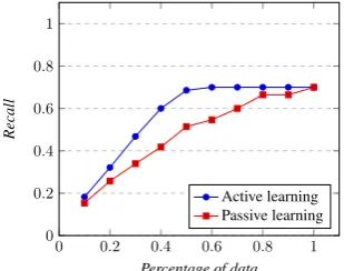
Figure 9 shows the recall when we choose ex-amples to be linearly independent in this way in comparison to when we choose examples ran-domly. The active learning scheme requires half as many labeled examples as the passive scheme to reach the same recall. In general, it takes rank(S) ≤ nexamples to obtain the same recall as having labeled all nexamples. Of course, the precision of both systems is 100%.
5.3 Paraphrasing
Another side benefit of the linear system relax-ation (Section 3.3) is that we can easily parti-tion the safe setFLS(8) into subsets of utterances
which are paraphrases of each other. Two utter-ances are paraphrase of each other if both map to the same logical form, e.g., “Texas’s capital” and “capital of Texas”. Given a sentencex∈ FLS, our
goal is to find all of its paraphrases inFLS.
As explained in Section 3.3, we can represent each inputxas a linear combination ofSfor some coefficientsα ∈ Rn: x =α>S. We want to find
allx0 ∈ FLS such thatx0 is guaranteed to map to
the same output asx. We can representx0=β>S
for some coefficientsβ ∈ Rn. The outputs forx
andx0 are thusα>T andβ>T, respectively. Thus
we are interested inβ’s such thatα>T =β>T, or
in other words,α−β is in the null space ofT>.
LetBbe a basis for the null space ofT>. We can
then writeα−β =Bvfor somev. Therefore, the set of paraphrases ofx∈ FLSare:
Paraphrases(x)def= {(α−Bv)>S:v ∈Rn}.
(9) 6 Discussion and related work
Our work is motivated by the semantic parsing task (though it can be applied to any set-to-set pre-diction task). Over the last decade, there has been much work on semantic parsing, mostly focusing on learning from weaker supervision (Liang et al., 2011; Goldwasser et al., 2011; Artzi and Zettle-moyer, 2011; Artzi and ZettleZettle-moyer, 2013), scal-ing up beyond small databases (Cai and Yates, 2013; Berant et al., 2013; Pasupat and Liang, 2015), and applying semantic parsing to other tasks (Matuszek et al., 2012; Kushman and Barzi-lay, 2013; Artzi and Zettlemoyer, 2013).
How-ever, only Popescu et al. (2003) focuses on preci-sion. They also obtain 100% precision, but with a hand-crafted system, whereas welearna semantic mapping.
The idea of computing consistent hypotheses appears in the classic theory of version spaces for binary classification (Mitchell, 1977) and has been extended to more structured settings (Vanlehn and Ball, 1987; Lau et al., 2000). Our version space is used in the context of the unanimity principle, and we explore a novel linear algebraic structure. Our “safe set” of inputs appears in the literature as the complement of the disagreement region (Hanneke, 2007). They use this notion for active learning, whereas we use it to support unanimous predic-tion.
There is classic work on learning classifiers that can abstain (Chow, 1970; Tortorella, 2000; Bal-subramani, 2016). This work, however, focuses on the classification setting, whereas we considered more structured output settings (e.g., for semantic parsing). Another difference is that we operate in a more adversarial setting by leaning on the una-nimity principle.
Another avenue for providing user confidence is probabilistic calibration (Platt, 1999), which has been explored more recently for structured predic-tion (Kuleshov and Liang, 2015). However, these methods do not guarantee precision forany train-ing set and test input.
In summary, we have presented the unanimity principle for guaranteeing 100% precision. For the task of learning semantic mappings, we lever-aged the linear algebraic structure in our prob-lem to make unanimous prediction efficient. We view our work as a first step in learning reli-able semantic parsers. A natural next step is to explore our framework with additional modeling improvements—especially in dealing with con-text, structure, and noise.
Reproducibility. All code, data, and
experiments for this paper are avail-able on the CodaLab platform at https: //worksheets.codalab.org/worksheets/ 0x593676a278fc4e5abe2d8bac1e3df486/.
Acknowledgments. We would like to thank the
References
Y. Artzi and L. Zettlemoyer. 2011. Bootstrap-ping semantic parsers from conversations. In Em-pirical Methods in Natural Language Processing (EMNLP), pages 421–432.
Y. Artzi and L. Zettlemoyer. 2013. Weakly supervised learning of semantic parsers for mapping instruc-tions to acinstruc-tions. Transactions of the Association for Computational Linguistics (TACL), 1:49–62. A. Balsubramani. 2016. Learning to abstain from
bi-nary prediction.arXiv preprint arXiv:1602.08151. J. Berant, A. Chou, R. Frostig, and P. Liang. 2013.
Semantic parsing on Freebase from question-answer pairs. InEmpirical Methods in Natural Language Processing (EMNLP).
Q. Cai and A. Yates. 2013. Large-scale semantic pars-ing via schema matchpars-ing and lexicon extension. In
Association for Computational Linguistics (ACL). C. K. Chow. 1970. On optimum recognition error and
reject tradeoff. IEEE Transactions on Information Theory, 16(1):41–46.
R. M. Freund, R. Roundy, and M. J. Todd. 1985. Iden-tifying the set of always-active constraints in a sys-tem of linear inequalities by a single linear program. Technical report, Massachusetts Institute of Tech-nology, Alfred P. Sloan School of Management. D. Goldwasser, R. Reichart, J. Clarke, and D. Roth.
2011. Confidence driven unsupervised semantic parsing. InAssociation for Computational Linguis-tics (ACL), pages 1486–1495.
S. Hanneke. 2007. A bound on the label complexity of agnostic active learning. InInternational Confer-ence on Machine Learning (ICML), pages 353–360. R. J. Kate, Y. W. Wong, and R. J. Mooney. 2005. Learning to transform natural to formal languages. InAssociation for the Advancement of Artificial In-telligence (AAAI), pages 1062–1068.
V. Kuleshov and P. Liang. 2015. Calibrated structured prediction. InAdvances in Neural Information Pro-cessing Systems (NIPS).
N. Kushman and R. Barzilay. 2013. Using semantic unification to generate regular expressions from nat-ural language. InHuman Language Technology and North American Association for Computational Lin-guistics (HLT/NAACL), pages 826–836.
T. Kwiatkowski, L. Zettlemoyer, S. Goldwater, and M. Steedman. 2010. Inducing probabilistic CCG grammars from logical form with higher-order uni-fication. InEmpirical Methods in Natural Language Processing (EMNLP), pages 1223–1233.
T. A. Lau, P. Domingos, and D. S. Weld. 2000. Version space algebra and its application to programming by demonstration. InInternational Conference on Ma-chine Learning (ICML), pages 527–534.
P. Liang, M. I. Jordan, and D. Klein. 2011. Learn-ing dependency-based compositional semantics. In
Association for Computational Linguistics (ACL), pages 590–599.
C. Matuszek, N. FitzGerald, L. Zettlemoyer, L. Bo, and D. Fox. 2012. A joint model of language and perception for grounded attribute learning. In Inter-national Conference on Machine Learning (ICML), pages 1671–1678.
S. Mei and X. Zhu. 2015. Using machine teaching to identify optimal training-set attacks on machine learners. InAssociation for the Advancement of Ar-tificial Intelligence (AAAI).
T. M. Mitchell. 1977. Version spaces: A candidate elimination approach to rule learning. In Interna-tional Joint Conference on Artificial Intelligence (IJ-CAI), pages 305–310.
B. Nelson, M. Barreno, F. J. Chi, A. D. Joseph, B. I. Rubinstein, U. Saini, C. Sutton, J. Tygar, and K. Xia. 2009. Misleading learners: Co-opting your spam filter. InMachine learning in cyber trust, pages 17– 51.
P. Pasupat and P. Liang. 2015. Compositional semantic parsing on semi-structured tables. InAssociation for Computational Linguistics (ACL).
J. Platt. 1999. Probabilistic outputs for support vec-tor machines and comparisons to regularized likeli-hood methods. Advances in Large Margin Classi-fiers, 10(3):61–74.
A. Popescu, O. Etzioni, and H. Kautz. 2003. Towards a theory of natural language interfaces to databases. In International Conference on Intelligent User In-terfaces (IUI), pages 149–157.
H. Shimodaira. 2000. Improving predictive inference under covariate shift by weighting the log-likelihood function. Journal of Statistical Planning and Infer-ence, 90:227–244.
F. Tortorella. 2000. An optimal reject rule for bi-nary classifiers. InAdvances in Pattern Recognition, pages 611–620.
K. Vanlehn and W. Ball. 1987. A version space ap-proach to learning context-free grammars. Machine learning, 2(1):39–74.
Y. W. Wong and R. J. Mooney. 2007. Learning synchronous grammars for semantic parsing with lambda calculus. InAssociation for Computational Linguistics (ACL), pages 960–967.