Munich Personal RePEc Archive
The relationship between energy
consumption, financial development and
economic growth: an evidence from
Malaysia based on ARDL
Malik, Meheroon Nisa Abdul and Masih, Mansur
INCEIF, Malaysia, INCEIF, Malaysia
30 December 2017
Online at
https://mpra.ub.uni-muenchen.de/86374/
The relationship between energy consumption, financial development and economic growth: an evidence from Malaysia based on ARDL
Meheroon Nisa Abdul Malik 1 and Mansur Masih2
Abstract
This study aims to examine the short-run and long-run relationship between economic growth,
energy consumption, financial development, capital formation and population by using data set of
Malaysia for the period 1971–2014. An emerging economy like Malaysia has high energy consumption which is intensified by its growing population. Economic growth and energy
consumption in Malaysia have been rising over the past several years. The motivation to this study
is related to four policy objectives of Malaysia; economic growth, financial development, energy
conservation and reduction on pollution. The auto regressive distributed lag (ARDL) bounds
testing approach to test the long run relationship among the variables, while short run dynamics
were investigated using the Vector Error Correction Model (VECM). Variance decomposition
(VDC) technique was used to provide Granger causal relationship between the variables.The
findings suggest that energy consumption is influenced by economic growth and financial
development, both in the short and the long run. The population–energy relationship however only holds in the long run. The results have important policy implications for balancing economic
growth vis-à-vis energy consumption for Malaysia, and other emerging nations to explore new and
alternative sources of energy to meet the rising demand of energy to sustain economic growth.
Key words: GDP, Energy consumption, Financial Development, Capital, Population Growth,
Malaysia
1
Graduate student in Islamic finance at INCEIF, Lorong Universiti A, 59100 Kuala Lumpur, Malaysia.
2Corresponding author, Professor of Finance and Econometrics, INCEIF, Lorong Universiti A, 59100 Kuala Lumpur, Malaysia.
1.0Introduction
The relationship between economic growth and energy consumption has been one of the most
pursued areas of research over the past decades. Numerous studies have investigated the causal
relationship between energy consumption and economic growth but the evidences have been
inconclusive. As the pursuit for economic prosperity in the emerging nations intensifies, the
significance of the subject is expected to gain its momentum. Energy is an essential basis for social
and economic development. The increase in vehicles and domestic equipments contributed by the
growth in population has led to a significant increase in energy demand. Furthermore, the energy
used in the production of goods and services has also been increasing in tandem with the economic
growth.
Numerous researchers have focused on examining the relationship between electricity
consumption and economic growth including Squalli (2007), Apergis and Payne (2011), Shahbaz
et al. (2013), Wolde-Rufael (2014), Rafindadi and Ozturk (2016) and Sarwar et al. (2017). Energy
is a relevant factor of domestic production and, hence, economic growth (Costantini and Martini,
2010) and any shortages may cause disruption to the output (GDP) and economic growth of a
nation (Shahbaz and Ali, 2016). The significance of the causal relationship between the energy
consumption and economic growth has brought about energy policy implications for the
policymakers especially energy conservation policies. Policies should be developed to avoid
energy wastage and reduce consumption where possible (Shahbaz and Ali, 2016).
Frankel and Romer (1999) pointed out that financial development in a country may attract foreign
direct investment (FDI) and in turn can, increase the level of economic growth. However, Jensen
(1996) found that financial development may lead to increased industrial activities which may lead
to industrial pollution as observed in China from 1953 to 2006. Ang (2008a) pointed out that
financial deepening in Malaysia leads to higher FDI inflows and Tamazian and Rao (2010) found
that increase in FDI inflows and R&D activities can reduce environmental pollution. Moreover,
the limited supply of world oil and natural gas (source of energy) potentially pose a threat to the
economic growth. This has brought about discussion on the need for alternate energy sources and
the incentive for research and development in this area of concern supported by government grants
and government policy.
This area of study on the relationship between energy consumption, financial development and
(1981) and, Engle and Granger (1987), Autoregressive Distributed Lag (ARDL) cointegration
technique or bound test of cointegration (Pesaran et al. 2001) and, Johansen and Juselius (1990)
cointegration techniques have become the solution to determining the long run relationship
between series that are non-stationary, as well as reparameterizing them to the Error Correction
Model (ECM).The objective of this paper is to examine the long run relationship between energy
consumption, financial development, economic growth, capital formation and population for
Malaysia by implementing the autoregressive distributed lag (ARDL) approach to cointegration;
and test the direction of causality using the Vector Error Correction Models (VECM).
Industrialization of Malaysia in the 1970s and 1980s has contributed to its rapid economic growth,
accompanied by significant improvement in its financial system. As illustrated n Figure 1, the ratio
of domestic credit to GDP increased from 24% in 1970 to 69% in 1980 and peaked at 163% of
GDP in 1997. Malaysia’s financial sector and its economy were severely affected by the Asian
financial crisis explaining the negative GDP growth of 7.4% in 1998 but rebound quickly in 1999.
The ratio of domestic credit to GDP has been declining since the Asian financial crisis and reached
109% of GDP in 2007. Market capitalization as a % of GDP also increased from 61% in 1981 to
321% in 1993 but went down to 82% of GDP during the Asian financial crisis in 1998.
Today, Malaysia is the third largest economy in Southeast Asia and the 35th largest economy in
the world. The government's development plans under the Tenth Malaysia Plan is largely centered
on accelerating economic growth through the three selected sectors (agriculture, manufacturing
and services) of the economy and building infrastructure to support these sectors. Malaysia prides
of being the highest growth economy amongst the emerging nations.
Studies conducted have validated the correlation between energy consumption and economic
growth but the causality direction between them is still outstanding. Does energy consumption
lead to economic growth or does economic growth promote energy consumption?
Given that the three major public policy goals of Malaysia are economic growth, financial
development and population growth, policymakers is interested to understand the long and short
run causality among the series and their direction which will aid in their policy making decision.
2.1 Theoretical Perspectives on Energy Consumption and Economic Growth
Studies conducted have validated the correlation between energy consumption and economic
growth but the causality direction between them is still outstanding. Does energy consumption
lead to economic growth or does economic growth promote energy consumption? The study of
interaction between economic activities and energy consumption was first published in the 1950s
by Mason (1955) and Frank (1959). The studies of Kraft and Kraft (1978) found unidirectional
causality between energy consumption and economic growth in the US market for the period 1947
to 1974. The interest in this topic has lead to many more studies done including Grossman and
Krueger (1995) and Selden and Song (1994), Akarca and Long (1980), Erol and Yu (1988), Masih
and Masih (1996), Aqeel and Butt (2001), Soytas and Sari (2003), Lee (2006), Huang et al. (2008),
Narayan and Smyth (2008), Bowden and Payne (2009), Lee and Chien (2010), Shahbaz and Lean
(2012a) and Shahbaz and Feridun (2012).
Although economic theories do not explicitly state a relationship between these variables,
theoretically the possible directions of causality can be explained by supply-leading and
demand-following hypothesis (Patrick, 1966). The supply-leading hypothesis infers a causal relationship
from energy consumption to economic growth i.e. energy consumption will lead to economic
growth. The demand-following hypothesis infers the opposite i.e. economic growth leads to energy
consumption. Studies found there is a relationship between energy consumption and economic
growth.
McKinnon (1973), King and Levine (1993a, b), Neusser and Kugler (1998), Darrat (1999), Levine,
Loayza and Beck (2000), Fase and Abma (2003), Christtopoulos and Tsionas (2004), Chang and
Caudill (2005), Rousseau and Vuthipadadorn (2005), Apergis and Payne (2009), Ozturk et al.
(2010), Ouedraogo (2013) and Aslan et al. (2014b) validated the growth hypothesis i.e. energy
consumption leads to economic growth while Gurley and Shaw (1967), Jung (1986), Lucas (1988),
Chandavarkar (1992), Liang and Teng (2006), Huang et al. (2008), Narayan et al. (2010), and
Kasman and Duman (2015) validated the conservative hypothesis i.e. that economic growth
influences energy consumption.
2.2 Empirical Review
The early empirical studies examined the energy-growth relationship using traditional stationary
(Akara and Long 1980, Yu and Wang 1984, Yu and Choi 1985). The long-term and short-term
relationship between energy consumption and economic growth has also been extensively
investigated using non-stationary approaches such as Vector Error Correction Model (VECM) to
test for Granger causality (Cheng and Lai 1997, Stern 2000, Narayan and Singh 2007, Ghosh 2009,
Iyke 2015 and Shabhaz et al. 2016). Narayan and Singh (2007), Ghosh (2009), Shahbaz and Lean
(2012) and Polemis and Dagoumas (2013) have sought to explain the electricity-growth nexus by
using symmetric causality tests.
Researcher such as Al-Iriani (2006), Narayan and Smith (2009), Costantini and Martini (2010),
Acaravci and Ozturk (2010), Wolde-Rufael (2014) and Karanfil and Li (2015) applied panel
methods to test for cointegration and Granger causality. Costantini and Martin (2010) and Acaravci
and Ozturk (2010) suggest use of panel techniques related to unit root, cointegration and causality
tests to eliminate the problems associated traditional unit root and cointegration tests.
Investigating electricity consumption - economic growth nexus in Pakistan, Shahbaz and Lean
(2012) found that electricity consumption has a positive effect on economic growth. The empirical
evidence provides a bi-directional Granger causality between electricity consumption and
economic growth in the short run suggesting that an electricity conservation policy may hinder
economic growth. In the case of Greece for the period 1970 to 2011, Polemis and Dagoumas (2013)
empirical findings revealed that Greece is an energy dependent country and energy conservation
policies by the policymakers can boost economic activity.
Narayan and Smyth (2009) found that incorporating other relevant factor in the production
function changes the causality direction. Shabhaz et al. (2013) argue that the exclusion of some
relevant variables in the empirical model clearly causes inconsistency in the econometric
specification and introduces biased estimates. This study considers the vital role of financial
development in production. Financial development has a positive effect on energy consumption
which is positively related to economic growth (Sadorski 2011b, Aslan et al. 2014, Rashid and
Yousaf 2015 for among others). Financial development may contribute to economic growth
directly and indirectly via capitalization (Shahbaz et al. 2017). Financial development affects
electricity consumption via consumer, wealth and business effects (Sardosky 2010, Shahbaz and
Lean 2012). According to Sadorski (2011b), this positive causality can be explained by three
confidence effect (known as the wealth effect). Financial development is measured by banking
variables such as bank deposits, financial system deposits and liquid liabilities.
3.0. Data
We have taken annual data from the World Development Indicator (WDI) published by the World
Bank for the period 1971–2014. The study comprises of time series data on GDP growth (annual percentage), energy use (kg of oil equivalent), domestic credit to private sector (percentage of
GDP), gross fixed capital formation (annual percentage growth) and population growth (annual
percentage) of Malaysia. These variable has been used in numerous studies including Soytas and
Sari (2009), Menyah and Rufael (2010), Shahbaz and Lean (2012), Dogan (2015b), and
Streimikienne and Kasperowicz (2016). There are bank-based and market-based financial
indicators to measure financial development. We have applied the commonly used domestic credit
as a % of GDP as a proxy for financial development (Clarke et al, 2006; Ang, 2010; Shahbaz and
Islam, 2011; Baligh and Piraee, 2013; Naceur and Zhang, 2016; and others).
As explained in the earlier section, economic growth also relies on other important inputs such as
financial development. Financial development is crucial in its role in sustaining energy efficient
technology (Shahbaz et al. 2011 and Tang et al. 2013) in enhancing domestic production and
investments in reducing greenhouse gases emissions. We included capital formation variable as
empirical evidence suggest that capital facilitates the transition from fossil fuels to alternative
renewable energy sources (Best, 2017).
The description of each variable is summarized below:
Gross domestic product (GDP) in annual percentage growth rate of GDP at market prices based on constant local currency
Energy consumption (ENE) measured in kg of oil equivalent per capita
Domestic credit to the private sector per capita is a measure of financial development Gross fixed capital formation per capita is a proxy for capital
Population growth (annual %)
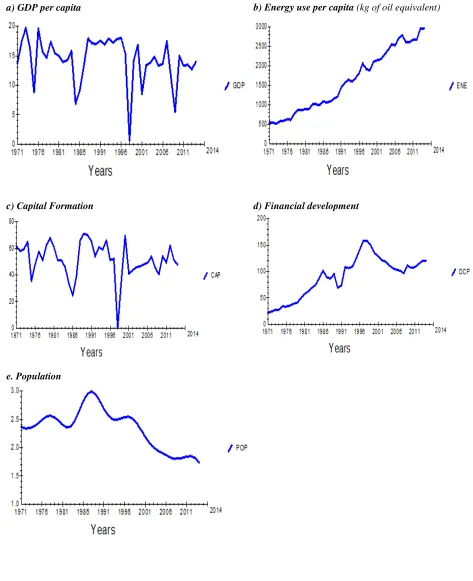
Figure 1 displays the time trend of the variables. The plot for GDP and CAP shows a close
relationship between the two variables and a steep in 1998 i.e. during the Asian Financial Crisis.
displayed in figure 1. Detailed data descriptions, sources and transformations are provided in the
appendix 1.
We aim to explore whether changes in the economic growth – energy consumption relationship are dependent to changes in the domestic credit to the private sector (DCP) and capital (CAP)
which was used as a proxy for financial development. We perform standard time series
econometrics methodologies: unit root tests and cointegration analysis. If a long-run relationship
[image:9.612.143.471.238.400.2]does exist, we can apply error correction modeling technique to ascertain the causal direction.
Figure 1: Trends in GDP, ENE, CAP, DCP AND POP for Malaysia from 1971 to 2014
a) GDP per capita b) Energy use per capita (kg of oil equivalent)
c) Capital Formation d) Financial development
4.0 Methodology
This paper employs the ARDL bounds testing cointegration approach to inspect whether a long
run dynamic relationship exists between GDP, energy consumption, financial growth, capital
formation and population growth. Various approaches have been applied to test the presence of
cointegration between variables in numerous studies and are explained in this section.
4.1 Unit Root / Stationarity Tests
A non-stationary time series is a stochastic process with unit roots or structural breaks. The
presence of a unit root indicates that a time series under consideration is non-stationary and the
absence a unit root indicates time series is stationary. The unit roots test is required to ascertain
the number of times a variable has to be differenced to achieve stationarity. A variable Y, is said
to be integrated of order d, I(d)] if it attained stationarity after differencing d times (Engle and
Granger, 1987). There are various methods of testing unit roots including Durbin-Watson (DW)
test, Dickey-Fuller test(1979)(DF), Augmented Dickey-Fuller(1981) (ADF) test, Philip-Perron
(1988) (PP) test and Kwiatkowski-Phillips-Schmidt-Shin (1992) (KPSS).
Standard unit root tests were used to assess if the variables were stationary: the Augmented Dickey
Fuller (ADF) test and Phillips-Perron (PP) test. Dickey and Fuller (1981) recommended the ADF
test to handle the AR(p) process in the variables. Perron (1989) noted that the unit root problem in
the series may cause biased empirical results. The ADF and PP tests the null hypothesis of a unit
root, against the alternative that it is stationarity. The ADF test adjusts the DF test to take care of
possible autocorrelation in the error terms by adding the lagged difference term of the dependent
variable. The PP test also takes cares of the autocorrelation in the error term and heteroscedasticity.
𝐇𝟎 : p1 =0 (p1 ∼ I(1)), i.e. not stationary
𝐇𝐀 : p1 < 0(p1∼ I(0)). i.e. it is stationary
When a series has a unit root (р1 =0), any shock to the data series is long lasting and hence suggest
stability in any policy formulation and implementation.
4.2 Tests for Lag Order Selection
The ARDL econometric specification relies on the assumption that the error term is serially
remove problems of serial correlation. However, given the relatively small sample size we should
avoid over-parameterization and be careful not to include too many lags. The Schwartz-Bayesian
Criterion (SBC), Akaike Information Criterion (AIC) or Hannan-Quinn Criterion (HQC). is used
to determine the optimal number of lags included in the test. AIC focuses on a large value of
log-likelihood and hence chooses a higher order of lags, whereas SBC is concerned with
over-parameterization and selects a lower order of lags.
4.3 ARDL Model to Test Cointegration
The ARDL bounds testing cointegration approach by Pesaran, Shin, and Smith (2001) to examine
the existence of a long run dynamic relationship between GDP, energy consumption, financial
development, capital formation and population growth. Researchers have applied various
approaches to test the presence of cointegration between variables in their studies. Two most
common approaches used is the Engle and Granger test (Engle and Granger, 1987) for bivariate
data and Johansen test (Johansen and Juselius, 1990) when multivariate. Both tests require that all
the series should be integrated at the order of integration I(1). Engle-Granger test for one
cointegrating relationship and Johansen test allows for multiple cointegrating relationships.
The ARDL bounds testing procedure involves two stages; first to test for the existence of a
long-run relationship between the variables and second to estimate the coefficients of the long-long-run
relations and make inferences about their values. The calculated F-statistic is compared against the
upper critical bound (UCB) and lower critical bound (LCB) provided by Pesaran et al. (2001)
which correspond to the assumptions that the variables are I(0) and I(1) respectively. If the
computed F-statistic is greater than the UCB value, then the H0 is rejected (the variables are
cointegrated). If the F-statistic is below the LCB value, then the H0 cannot be rejected (there is no
cointegration among the variables). If it falls between the LCB and UCB value, the result of the
inference is inconclusive.
cointegration is inconclusive if it is between the UCB and the LCB. While these asymptotic critical
values are reliable for large samples. For smaller samples ranging from 30 to 80 observations,
Narayan (2005) provides F-test the critical values bounds. The computed F-tests in this subsection
will be compared against both sets of critical values.
The ARDL bound testing is more suitable than other traditional cointegration tests as it corrects
relationships of variables. The ARDL method can be used for data series integrated at the order
I(0) or I(1) and calculates short run and long run parameters simultaneously. The ARDL approach
is superior in small samples to other single and multivariate cointegration methods (Narayan,
2005).
The ARDL model specifications of the functional relationship between Gross Domestic Product
(GDP), Energy Consumption (ENE), Financial Growth (DCP), Capital Formation (CAP) and
Population Growth (POP) is shown below:
∆𝐺𝐷𝑃𝑡 = 𝑎0+ ∑𝑝𝑡=1𝑏1∆𝐺𝐷𝑃𝑡−1 + ∑𝑝𝑡=1𝑐1∆𝐸𝑁𝐸𝑡−1 + ∑𝑝𝑡=1𝑑1∆𝐷𝐶𝑃𝑡−1 + ∑𝑝𝑡=1𝑒1∆𝐶𝐴𝑃𝑡−1 + + ∑𝑝𝑡=1𝑓1∆𝑃𝑂𝑃𝑡−1 + 𝛿1𝐺𝐷𝑃𝑡−1 + 𝛿2𝐸𝑁𝐸𝑡−1 + 𝛿3𝐷𝐶𝑃𝑡−1 + 𝛿4𝐶𝐴𝑃𝑡−1 + 𝛿5𝑃𝑂𝑃𝑡−1 + 𝜀𝑡
∆𝐸𝑁𝐸𝑡 = 𝑎0+ ∑𝑝𝑡=1𝑏1∆𝐺𝐷𝑃𝑡−1 + ∑𝑝𝑡=1𝑐1∆𝐸𝑁𝐸𝑡−1 + ∑𝑝𝑡=1𝑑1∆𝐷𝐶𝑃𝑡−1 + ∑𝑝𝑡=1𝑒1∆𝐶𝐴𝑃𝑡−1 + + ∑𝑝𝑡=1𝑓1∆𝑃𝑂𝑃𝑡−1 + 𝛿1𝐺𝐷𝑃𝑡−1 + 𝛿2𝐸𝑁𝐸𝑡−1 + 𝛿3𝐷𝐶𝑃𝑡−1 + 𝛿4𝐶𝐴𝑃𝑡−1 + 𝛿5𝑃𝑂𝑃𝑡−1 + 𝜀𝑡
∆𝐷𝐶𝑃𝑡= 𝑎0+ ∑𝑝𝑡=1𝑏1∆𝐺𝐷𝑃𝑡−1 + ∑𝑝𝑡=1𝑐1∆𝐸𝑁𝐸𝑡−1 + ∑𝑝𝑡=1𝑑1∆𝐷𝐶𝑃𝑡−1 + ∑𝑝𝑡=1𝑒1∆𝐶𝐴𝑃𝑡−1 + + ∑𝑝𝑡=1𝑓1∆𝑃𝑂𝑃𝑡−1 + 𝛿1𝐺𝐷𝑃𝑡−1 + 𝛿2𝐸𝑁𝐸𝑡−1 + 𝛿3𝐷𝐶𝑃𝑡−1 + 𝛿4𝐶𝐴𝑃𝑡−1 + 𝛿5𝑃𝑂𝑃𝑡−1 + 𝜀𝑡
∆𝐶𝐴𝑃𝑡 = 𝑎0+ ∑𝑝𝑡=1𝑏1∆𝐺𝐷𝑃𝑡−1 + ∑𝑝𝑡=1𝑐1∆𝐸𝑁𝐸𝑡−1 + ∑𝑝𝑡=1𝑑1∆𝐷𝐶𝑃𝑡−1 + ∑𝑝𝑡=1𝑒1∆𝐶𝐴𝑃𝑡−1 + + ∑𝑝𝑡=1𝑓1∆𝑃𝑂𝑃𝑡−1 + 𝛿1𝐺𝐷𝑃𝑡−1 + 𝛿2𝐸𝑁𝐸𝑡−1 + 𝛿3𝐷𝐶𝑃𝑡−1 + 𝛿4𝐶𝐴𝑃𝑡−1 + 𝛿5𝑃𝑂𝑃𝑡−1 + 𝜀𝑡
∆𝑃𝑂𝑃𝑡 = 𝑎0+ ∑𝑝𝑡=1𝑏1∆𝐺𝐷𝑃𝑡−1 + ∑𝑝𝑡=1𝑐1∆𝐸𝑁𝐸𝑡−1 + ∑𝑝𝑡=1𝑑1∆𝐷𝐶𝑃𝑡−1 + ∑𝑝𝑡=1𝑒1∆𝐶𝐴𝑃𝑡−1 + + ∑𝑝𝑡=1𝑓1∆𝑃𝑂𝑃𝑡−1 + 𝛿1𝐺𝐷𝑃𝑡−1 + 𝛿2𝐸𝑁𝐸𝑡−1 + 𝛿3𝐷𝐶𝑃𝑡−1 + 𝛿4𝐶𝐴𝑃𝑡−1 + 𝛿5𝑃𝑂𝑃𝑡−1 + 𝜀𝑡
The ARDL cointegration test is testing the following hypotheses:
𝐇𝟎 = 𝛿1= 𝛿1 = 𝛿2 = 𝛿3 = 𝛿4= 𝛿5= 0; (there is no cointegration i.e. no long run relationship
between the variables)
𝐇𝐀 = 𝛿1 ≠ 𝛿2 ≠ 𝛿3 ≠ 𝛿4≠ 𝛿5≠ 0 (i.e. there is cointegration or long run relationship between
the variables)
This is tested in each of the models as specified by the number of variables and denoted as follows:
FX (X1│Y1… . Yk)
FY (Y1│ X1… . Xk)
The hypothesis is tested by means of the F- statistic (Wald test).
The ARDL model establishes the existence of a long-run relationship between economic growth
and energy consumption but it does not explain the short-run dynamics that brings about the
long-run equilibrium. We use the t-statistic of the error correction model (ECM) to test the causality of
the variables while the coefficient of the ECT from the ECM indicates the speed of adjustment of
the dependent variable towards its long run equilibrium. ECM identifies which variable is
exogenous (strong) and which is endogenous (weak) If the value is zero, then there exists no
long-run relationship. If the speed of adjustment value is between -1 and 0, then there exists partial
adjustment.
The ECM tests the following hypothesis:
𝐇𝟎: The variable is exogeneous
𝐇𝐀: The variable is endogenous
4.5 Variance Decomposition (VDC)
ECM model only provides information about the absolute endogeneity or exogeneity. The relative
degree of endogeneity or exogeneity of the variables can be determined using the variance
decomposition (VDC) test. The VDCs provides a decomposition of the variance of the forecast
errors of each of the variables in the VAR (vector auto regression) at different horizons into
proportions attributable to shocks from each variable in the system including its own. The variable
that depends most on its own past is the most exogenous. To affect the endogenous variable,
policymakers will set the exogenous variable as an intermediate target.
From the two types of VDCs, generalized VDC is preferred as it is invariant to the ordering of the
variables and is self-dependence in response to shocks. The orthogonalized VDCs however are not
unique and are dependent on the particular ordering of the variables in the VAR. It also assumes
that when a particular variable is shocked, all other variables in the model are switched off.
generalized forecast error VDC permits one to make robust correlation of the
strength, size and persistence of shocks from one equation to another (Payne, 2002)
4.6 Impulse Response Functions (IRFs)
Impulse response function (IRF) displays the impact of a shock on one variable to others and
information to VDC in graphical form. When there is a shock to endogenous variable, the
exogenous variables are highly affected as it takes shorter period to normalize.
5.0 Findings and Discussion
5.1 Unit Root Tests
The result for the five variables from both ADF and PP tests is summarized in Table 1a and Table
1b below. The differenced form of variables is integrated of order two, I(2) indicating the existence
of a unit root. The ADF and PP test found the series to be non-stationary at level form and
[image:15.612.73.308.454.552.2]stationary at different form
Table 1a: Empirical results of a Unit Root Tests (ADF)
Level Form Difference Form
VARIABLE T-STAT. C.V. RESULT VARIABLE T-STAT. C.V. RESULT
LGDP -3.1038 -3.5313 Non-stationary DGDP -3.6321 -3.5348 Stationary
LCAP -2.5497 -3.5313 Non-stationary DCAP -3.7553 -3.5348 Stationary
LDCP -2.2450 -3.5313 Non-stationary DENE -6.0034 -3.5348 Stationary
LPOP -.86131 -3.5313 Non-stationary DDCP -2.8664 -3.5348 Non-stationary
LENE -2.1356 -3.5313 Non-stationary DPOP -3.2236 -3.5348 Non-stationary
Difference Form (Second)
VARIABLE T-STAT. C.V. RESULT
DGDP -6.620035 -3.615588*** Stationary
DCAP -4.961703 -3.626784*** Stationary
DENE -6.452480 -3.615588*** Stationary
DDCP -10.30228 -3.605593*** Stationary
DPOP -3.562778 -2.948404** Stationary
Table 1b: Empirical results of a Unit Root Tests (PP)
Level Form First Difference Form
VARIABLE
T-STAT. C.V. RESULT VARIABLE T-STAT. C.V. RESULT
DGDP -6.307457 -3.592462*** Stationary DGDP -30.20152 -3.596616*** Stationary
DCAP -6.166937 -3.592463*** Stationary DCAP -37.38675 -3.596616*** Stationary
DENE -1.643071 -2.603944* Non-stationary DENE -7.145207 -3.596616*** Stationary
DDCP -2.659923 -2.603944* Stationary DDCP -5.782205 -3.596616*** Stationary
DPOP -0.230937 -2.603944* Non-stationary DPOP -2.416331 -2.604867* Non-stationary
*** Show significance at the 1% level ** Show significance at the 5% level * Show significance at the 10% level
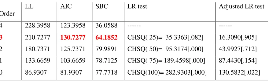
5.2 Tests for Lag Order Selection
The corresponding value to the highest AIC in Table 2 suggest lag order of 3.
Table 2: Optimal Lag Selection
Order
LL AIC SBC LR test Adjusted LR test
4 228.3958 123.3958 36.0588 --- ---
3 210.7277 130.7277 64.1852 CHSQ( 25)= 35.3363[.082] 16.3090[.905]
2 180.7371 125.7371 79.9891 CHSQ( 50)= 95.3174[.000] 43.9927[.712]
1 133.6659 103.6659 78.7125 CHSQ( 75)= 189.4598[.000] 87.4430[.154]
0 86.9307 81.9307 77.7718 CHSQ(100)= 282.9303[.000] 130.5832[.022]
AIC=Akaike Information Criterion SBC=Schwarz Bayesian Criterion
5.3 ARDL Approach to Cointegration
The results for F-test for cointegration are presented in Table 3. Overall, we find sufficient
[image:16.612.79.519.366.499.2]Table 3: Empirical results of ARDL Tests – F-test
Models F-statistics
FLGDP (LGDP | LENE, LDCP, LCAP, LPOP) 3.5744***
FLENE (LENE | LGDP, LDCP, LCAP, LPOP) 2.5867
FLDCP (LDCP | LGDP, LENE, LCAP, LPOP) 1.2391
FLCAP (LCAP | LGDP, LENE, LDCP, LPOP) 3.0260*
FLPOP (LPOP | LGDP, LENE, LDCP, LCAP) 0.81684
*** Show significance at the 1% level ** Show significance at the 5% level * Show significance at the 10% level
F-stat Significance LCB UCB 10% 1.825 2.943 5% 2.157 3.340 1% 2.903 4.261
The ARDL bound test result above reveals that the calculated F-statistics exceeded the upper
critical value in two out of six equations tested at standard acceptable significance levels. We
conclude that the variables are cointegrated and there is long-run theoretical relationship \among
economic growth, energy consumption, financial growth, capital formation and population growth
of Malaysia for the period of 1976-2014.
Table 4: Empirical results of ARDL Tests – F-test
K LGDP
LENE .47154**
LDCP -.42195**
LCAP .47089***
LPOP 1.3287***
INPT -1.9619
[image:17.612.74.255.478.638.2]The results in above table reveals that there is a positive long run relationship between energy
consumption and GDP and highly significant at 5%. This implies that a 1% increase in energy
consumption would increase GDP by 4.72% and supports the numerous studies that found positive
relationship between energy consumption and GDP (Khan and Qayyum, 2006). Hence, energy
consumption is crucial in generating economic growth.
Similarly, there is positive long run relation between fixed capital formation and GDP and
population growth and GDP. Both relationships are highly significant at 1%. This implies that a
1% increase in fixed capital formation or population growth would increase GDP by 4.71% and
13.79% respectively. The positive long run relationship does not hold for Domestic credit to the
private sector (proxy for financial growth) as our findings reveal that an increase in financial
growth leads to negative economic growth.
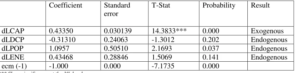
5.4 Error Correction Model (ECM)
The result of T-stat and the causality coefficient of ECM test are shown in table 5. We found that
only CAP and POP is significant and thus is endogenous. Meanwhile GDP, DCP and ENE are
[image:18.612.75.558.457.576.2]found to be exogenous (not statistically significant in ECM model).
Table 5: Error Correction Model
Dependent Variable = Economic Growth
Coefficient Standard error
T-Stat Probability Result
dLCAP 0.43350 0.030139 14.3833*** 0.000 Exogenous
dLDCP -0.31310 0.24063 -1.3012 0.202 Endogenous
dLPOP 1.0957 0.50510 2.1693 0.037 Endogenous
dLENE 0.43468 0.28846 1.5069 0.141 Endogenous
ecm (-1) -1.000 0.000 -7.1735 0.000
*** Show significance at the 1% level ** Show significance at the 5% level * Show significance at the 10% level
The results imply that when we shock capital formation the exogenous variables (GDP, ENE, DCP
and POP) will affected. Hence, should the policymakers wish to control the exogenous variables
e.g. energy consumption, they should control the fixed capital formation in the country.
The exogenous variables would receive market shocks and transmit the effects of those shocks to
equilibrium if that variable is shocked. The coefficient of the error correction term i.e. ecm(-1) is
negative and statistically significant suggesting that it would take a long time for the equation to
return to equilibrium once it has been shocked.
ECM model only distinguishes the absolute endogeneity and exogeniety of a variable but does
indicate the relative degree of endogeneity or exogeneity. This can be identified using the variance
decomposition technique (VDC).
4.5 Variance Decomposition (VDC)
The results from the VDC test is shown in table 6. The variable ranked higher is the leading
variable, and should targeted by policymakers. We include three time horizons, 5, 10 and 15, to
depict the short-term, the medium-term and the long-term impact of shocks, respectively. As seen
in table 6, capital formation is the most exogenous while energy consumption is most endogenous
for time horizon 5 years. The standing of capital formation and energy growth remained throughout
the 15 years. However the standing of most endogenous variable changed to population growth in
10 years horizon and financial growth in 15 years horizon.
5.6 Impulse Response Functions (IRFs)
Figure 2 are the graph for IRFs for the period of 30 years. The graph explains that when the capital
is shock, we can see the fast response from the other four variables but normalizes after a certain
time horizon. Judging by the graph, GDP and CAP normalizes after 4 year horizon, ENE after 10
years horizon and DCP and POP takes more than 10 years to normalize after a ‘shock’. The endogenous variables are more affected and the exogenous variables are least affected.
Hence policymakers will make decision on GDP will influence the CAP as changes in CAP will
Table 6. Variance Decomposition (VDCs) for Horizon 5, 10 and 15
Horizon LGDP LCAP LDCP LPOP LENE TOTAL RANK
LGDP 5 21% 72% 5% 0% 1% 100% 2
LCAP 5 24% 70% 3% 0% 3% 100% 1
LDCP 5 33% 62% 4% 0% 0% 100% 4
LPOP 5 22% 65% 3% 5% 5% 100% 3
LENE 5 29% 67% 2% 2% 0% 100% 5
Horizon LGDP LCAP LDCP LPOP LENE TOTAL RANK
LGDP 10 27% 42% 18% 4% 9% 100% 2
LCAP 10 36% 59% 1% 1% 3% 100% 1
LDCP 10 25% 66% 5% 1% 2% 100% 3
LPOP 10 35% 54% 9% 0% 1% 100% 5
LENE 10 28% 67% 2% 1% 1% 100% 4
Horizon LGDP LCAP LDCP LPOP LENE TOTAL RANK
LGDP 15 32% 50% 15% 1% 2% 100% 2
LCAP 15 33% 44% 19% 0% 3% 100% 1
LDCP 15 27% 63% 2% 5% 2% 100% 5
LPOP 15 36% 37% 11% 14% 2% 100% 3
6.0 CONCLUSION AND POLICY IMPLICATIONS
This study investigated the relationship between economic growth, and energy consumption in
Malaysia using annual time series data for the period of 1976 – 2014. ARDL cointegration method developed by Shin et al. (2014) was applied and we tested the causal relationship between the
variables using VECM, VDCs and IRF tests. The empirical results provide evidence that the
variables are asymmetrically cointegrated. The finding of this study is crucial as it suggests that a
change in the energy consumption will affect the economic growth in Malaysia and the impact of
a reduction in energy consumption will have a larger effect compared to an increase in energy
consumption. Policymakers in Malaysia can influence the economic growth in Malaysia by
controlling the energy consumption of the nation. Government incentives in encouraging energy
saving behavior and development of alternate source of energy can lead to sustained economic
growth without impacting the production level of the nation.
The findings also revealed positive relationship between financial development and economic
growth, population growth and economic growth and capital formation and economic growth. The
coefficient and raking of capital formation suggest that this variable is most significant among the
variables in the study. Positive shock to capital formation will lead to higher long-term fiscal
investments in infrastructure development and hence increases economic growth in the long term.
We recommend that the policymakers in Malaysia to focus on improving fixed capital formation
and encourage larger sum of investment in infrastructure development for sustainable economic
growth.
Last not but least, the causality result recommends that to influence the GDP i.e. economic growth,
policymakers should impact capital formation to influence the economic growth in the short term,
medium and in the long run (5 to 15 years horizon). This can be done via not only infrastructure
upgrade but also policies to encourage capital investment. Perhaps including foreign direct
investment as a control variable may enhance the findings and strengthen the findings on the
Appendix 1: Data Transformations
Economic Growth LGDP=LOG(GDP)
DLGDP=LGDP – LGDP(-1)
Energy Consumption LENE = LOG(ENE)
DLENE = LENE – LENE(-1)
Financial Development LDCP = LOG(DCP)
DDCP = LDCP – LDCP(-1)
Capital Formation LCAP = LOG(CAP)
DCAP = LCAP – LCAP(-1)
Population LPOP = LOG(POP)
References
Akara, A., Long, T., 1980. On the relationship between energy and GNP: a re-examination. Journal of Energy Development 5, 326–331.
Al-Iriani, M.A., 2006. Energy–GDP relationship revisited: an example from GCC countries using panel causality. Energy Policy 34 (17), 3342–3350.
Ang, J.B., 2008. Economic development, pollutant emissions and energy consumption in Malaysia. Journal of Policy Modeling 30, 271–278.
Apergis, N., Payne, J., 2010. Renewable energy consumption and economic growth: evidence from a panel of OECD countries. Energy Policy 38(1), 656–660.
Apergis, N., Payne, J., 2011. A dynamic panel study of economic development and the electricity consumption-growth nexus. Energy Economics, 33(5), 770–781.
Arora, V., Shi, S., 2016. Energy consumption and economic growth in the United States. Applied Economics, 48, 3763-3773.
Aslan, A., Apergis, N., Topcu, M., 2014. Banking development and energy consumption: Evidence from a panel of Middle Eastern countries. Energy 72, 427-433.
Best, R., 2017. Switching towards coal or renewable energy? The effects of financial capital on energy transitions. Energy Economics, 63, 75-83.
Bhattacharya, M., Paramatti, S.R., Ozturk, I., Bhattacharya, S., 2016. The effect of renewable energy consumption on economic growth: Evidence from top 38 countries. Applied Energy, 162, 733-741.
Brock, W.A., Dechert, W.D., Scheinkman, J.A., LeBaron, B., 1996. A Test for Independence Based on the Correlation Dimension. Econometric Reviews 15, 197-235.
Chang, S.C., 2015. Effects of financial developments and income on energy consumption. International Review of Economics and Finance 35, 28-44.
Chen, S.-T., Kuo, H.-I., Chen, C.-C., 2007. The relationship between GDP and electricity consumption in 10 Asian countries. Energy Policy, 35(4), 2611–2621.
Cheng, B. S., Lai, T. W., 1997. An investigation of co-integration and causality between energy consumption and economic activity in Taiwan. Energy Economics, 19(4), 435–444.
Cheng, M., Chung, L., Tam, C-S., Yuen, R., Chan, S., Yu, I-W., 2012. Tracking the Hong Kong Economy. Hong Kong Monetary Authority, Occasional Paper 03/2012.
Chtioui, S., 2012. Does economic growth and financial development spur energy consumption in Tunisia? Journal of Economics and International Finance 4(7), 150-158.
Cole M.A., 2006. Does trade liberalisation increase national energy use? Economic Letters, 92, 108-112.
Costantini, V., Martini, C., 2010. The causality between energy consumption and economic growth: A multi-sectoral analysis using non-stationary cointegrated panel data. Energy Economics, 32(3), 591–603.
D. Dickey and W. Fuller, Likelihood Ratio Statistics for Autoregressive Time Series with a Unit Root,
Econometrica, 49, (1981), 1057-1072.
Fuinhas, J.A., Marques, A.C., 2012. Energy consumption and economic growth nexus in Portugal, Italy, Greece, Spain and Turkey: An ARDL bounds test approach (1965-2009). Energy Economics, 34(2), 511-517.
Ghosh S., 2009. Electricity supply, employment and real GDP in India: evidence from cointegration and Granger-causality tests. Energy Policy, 37, 2926-2929.
Granger, C.W.J., Yoon, G., 2002. Hidden cointegration. Working Paper, University of California, San Diego.
Pesaran, M. H. Shin, Y., Smith, R. J., 2001. Bounds testing approaches to the analysis of level relationships. Journal of Applied Econometrics, 16, 289–326.
Hatemi J.A., 2012. Asymmetric causality tests with an application. Empirical Economics, 43(1), 447-456.
Iyke, B., 2015. Electricity consumption and economic growth in Nigeria: A revisit of the energy growth debate. Energy Economics, 51, 166-176.
Jalil, A., Feridun, M., 2011. The impact of growth, energy and financial development on the environment in China: a cointegration analysis. Energy Economics 33, 284-291.
Kraft, J., Kraft, A., 1978. On the relationship between energy and GNP. Journal of Energy Development 3, 401–403
Lean, H.H., and Smyth, R., 2010. On the dynamics of aggregate output, electricity consumption and exports in Malaysia: Evidence from multivariate Granger causality tests. Applied Energy, 87, 1963-1971.
Mahalik, M.K., Mallick, H., 2014. Energy consumption, economic growth and financial development: exploring the empirical linkages for India. The Journal of Developing Areas 48(4), 139-159.
Masih, A.M.M., Masih, R., 1996. Energy consumption, real income and temporal causality: results from a multi-country study based on cointegration and error correction modeling techniques. Energy Economics
18, 165-183.
Narayan, P.K., Narayan, S., Popp, S., 2010. A note on the long-run elasticities from the energy consumption-GDP relationship. Applied Energy 87(3), 1054-1057.
Narayan, P.K., Smyth, R., 2009. Multivariate Granger causality between electricity consumption, exports and GDP: evidence from a panel of Middle Eastern countries. Energy Policy, 37, 229–236.
Omri, A., 2014. An international literature survey on energy-economic growth nexus: Evidence from country-specific studies. Renewable and Sustainable Energy Reviews, 38, 951-959.
Ouedraogo, N.S., 2013. Energy consumption and economic growth: evidence from the economic community of West African states (ECOWAS). Energy Economics 36, 637-647.
Ozturk, I., Acaravci, A., 2013. The long-run and causal analysis of energy, growth, openness and financial development on carbon emissions in Turkey. Energy Economics 36, 262-267.
Payne, J.E., 2010. A survey of the electricity consumption-growth literature. Applied Energy 87(3), 723– 731.
Polemis, M.L., Dagoumas, A.S., 2013. The electricity consumption and economic growth nexus: Evidence from Greece. Energy Policy, 62, 798-808.
Rafindadi, A., Ozturk, I., 2016. Effects of financial development, economic growth and trade on electricity consumption: Evidence from post-Fukushima Japan. Renewable and Sustainable Energy Reviews, 54, 1073-1084.
Salmanai, Doaa M., Atyab Eyad M., 2014. What is the role of Financial Development and Energy Consumption on Economic Growth? New Evidence from North African Countries. International Journal of Finance & Banking Studies IJFBS Vol.3 No.1, 2014 ISSN: 2147-4486.
Sarwar, S., Chen, W., Wahhed, R., 2017. Electricity consumption, oil price and economic growth: Global perspective. Renewable and Sustainable Energy Reviews, 76, 9-18.
Shahbaz, M. and Ali, A. (2016). Measuring Economic Cost of Electricity Shortage: Current Challenges and Future Prospects in Pakistan. Bulletin of Energy Economics, 4, 211- 223.
Shahbaz, M., Tang, C.F., Shahbaz, M.S., 2011. Electricity consumption and economic growth nexus in Portugal using cointegration and causality approaches. Energy Policy, 39, 3529- 3536.
Shahbaz, M., Van Hoang, T-H., Mahalik, M.K., Roubaud, D., 2017. Energy Consumption Financial Development and Economic Growth in India: New Evidence from a Nonlinear and Asymmetric Analysis. Energy Economics, 63, 199-212.
Shin, Y., Yu, B., Greenwood-Nimmo, M., 2014. Modelling asymmetric cointegration and dynamic multipliers in an ARDL framework. In: Horrace, W.C., Sickles, R.C., (Eds.), Festschrift in Honorof Peter Schmidt, Springer Science and Business Media, New York.
Singh, A. 1997. Financial liberalization, stock markets and economic development, Economic Journal 107, 771–782.
Squalli, J., 2007. Electricity consumption and economic growth: bounds and causality analyses of OPEC members. Energy Economics 29, 1192-1205.
Streimikiene, D., Kasperowicz, R., 2016. Review of economic growth and energy consumption: A panel cointegration analysis for EU countries. Renewable and Sustainable Energy Reviews. 59, 1545–1549
Tang, C. F., Tan, B. W., Ozturk, I., 2016. Energy consumption and economic growth in Vietnam. Renewable and Sustainable Energy Reviews, 54, 1506-1514.