Munich Personal RePEc Archive
Consistent and inconsistent choices
under uncertainty: The role of cognitive
abilities
Amador, Luis and Brañas-Garza, Pablo and Espín, Antonio
M. and Garcia, Teresa and Hernández, Ana
Loyola Behavioral Lab (Spain), Universidad Loyola Andalucía
(Spain), Universidad de Granada (Spain)
17 July 2019
Online at
https://mpra.ub.uni-muenchen.de/95178/
Consistent and inconsistent choices under
uncertainty: The role of cognitive abilities
1Luis Amador1, Pablo Brañas-Garza1, Antonio M. Espín1,2, Teresa García1,2,
Ana Hernández1
1 Loyola Behavioral Lab, Universidad Loyola Andalucía, Spain. 2 Universidad de Granada, Spain.
Abstract
There is an intense debate whether decision making under uncertainty is partially driven by cognitive abilities. The critical issue is whether choices arising from subjects with lower cognitive abilities are more likely driven by errors or lack of understanding than pure preferences for risk. The latter implies that the often argued link between risk preferences and cognitive abilities might be a spurious correlation. This experiment reports evidence from a sample of 556 participants who made choices in risk-related tasks about winning and losing money and completed three cognitive tasks, all with real monetary incentives: number-additions under time pressure (including incentive-compatible expected number of correct additions), the Cognitive Refection Test (to measure analytical/reflective thinking) and the Remote Associates Test (for convergent thinking). Results are unambiguous: none of our cognition measures plays any systematic role on risky decision making. Our data indeed suggest that cognitive abilities are negatively associated with noisy, inconsistent choices, which might have led to spurious correlations with risk preferences in previous studies.
JEL codes: D81, C91.
Keywords: decision making under uncertainty, cognitive abilities, online experiment.
I Introduction
Typically, experimental economists use lottery tasks to measure individuals’
preferences for risk. For instance, in the Holt and Laury (2002) mechanism, subjects have to choose between lottery A and B in 10 decisions (both lotteries with two possible outcomes and probabilities), while in Eckeland Grossman (2002) they have to choose among six gambles, all with a 0.5 probability of winning a higher prize. Generally speaking, Multiple Prices Lists (MPL) experimental devices such as the above may involve a lot of probability computation. It is often observed that about 15%–20% of the participants are
1 We thank Pedro Caldentey for coordinating the experiment. We also thank Behave4’s
inconsistent; a percentage that can increase dramatically in non-student samples (see Charness et al. 2013).
The truth is that lotteries or computations involving probabilities are not easy tasks. In fact, many brain areas related to cognition appear to be involved in probability calculus. In a sample of subjects making probabilistic choices, Berns et al. (2008) showed that brain responses (to probabilities) are consistent with nonlinear probability weighting. Indeed, they provided evidence for notable neural activity in a circumscribed network of brain regions that included the anterior cingulate and the visual, parietal and temporal cortices.
Assuming that decision making under uncertainty (DMU) requires an ability to compute probabilities, it follows that choices by subjects with lower Cognitive
Abilities (CAbs) might be partially the result of mistakes or lack of
understanding rather than pure taste for specific prospects (risk preferences).
However, if individuals are able to differentiate risky from non-risky prospects regardless of their innate capacity to evaluate probabilities—that is, even those endowed with low abilities can do it—then their choices reflect pure
preferences for risk. This question is not new and has been explored using
administrative, survey (incentivized and hypothetical) and experimental data (typically from the lab) on risk taking. In the following lines, we summarize the main findings for each of these three strands of the literature.
Administrative data
Christelis et al. (2010), Van Rooj et al. (2011), Grinblatt et al. (2011), Frisell et al. (2012), Cole et al. (2014), Beauchamp et al. (2017) and Angrisani and Casanova (2018) have studied the role of CAbs in risk-taking behavior in different contexts of life: stock market participation, alcohol consumption and smoking, saving, portfolio selection and violent crime. Such studies do not measure risk preferences in purpose-designed tasks, but simply observe behaviors or choices that serve as indirect observations of risk preferences. In this regard, Dohmen et al. consider that:
vary across contexts and studies. With a closer look at this variation, however, a pattern emerges. Cognitive ability tends to be positively correlated with avoidance of harmful risky situations and to be negatively correlated with risk aversion in advantageous situations. (2018: 120)
This might be indicating that high cognitive ability is associated with risk neutrality. According to these same authors (2018:120), “evidence for this emerges both from studies of behavior in risky situations, often conducted by psychologists and psychiatrists, and also from studies focused on economic decision-making” as, for example, stock market participation.
That said, since these studies use proxies that indirectly infer risk taking from observed behavior, it is difficult to draw firm conclusions about risk preferences. For instance, time is an important underlying factor beyond risk (i.e., volatility) in many of these decisions, thus time preferences may also determine savings, drug use and violent crime (Åkerlund et al. 2016, Bickel et al. 1999, Meier and Sprenger 2012). Moreover, the CAbs measures differ greatly from one study to another. For example, Christelis et al. (2010) employed math, verbal and recall tests and found similar results for each of the three measures; Angrisani and Casanova (2018) tested separately for
numeracy and “cognition” (episodic memory and fluid intelligence) and also
found similar relationships for the two types of measures, while Grinblatt et al. (2011) combined psychological tests assessing mathematical, verbal and logical skills into one composite score.
Survey data
ranking used for university entrance). Falk et al. (2018) developed the Global Preference Survey (GPS), an experimentally validated survey data set of time preference, risk preference, positive and negative reciprocity, altruism and trust of 80,000 people in 76 countries. They elicited risk preferences through a series of related quantitative questions (hypothetical lottery choice sequence using staircase method) as well as one qualitative question (self-assessment: willingness to take risks in general). The GPS also elicited a self-reported proxy for CAbs by asking people to assess themselves by the statement “I am
good at math” on an 11-point Likert scale.
Chapman et al. (2018) showed that participants with higher CAbs are more loss averse and less risk averse. Falk et al. (2018) confirmed that risk aversion is more pronounced for individuals with lower CAbs. Booth and Katic (2013) did not find a statistically significant correlation between CAbs and risk attitudes.
Again, however, the risk preferences as well as CAbs measures vary greatly from one study to another. In contrast to the above administrative data papers, these studies tend to combine their CAbs measures into one single variable rather than analyzing them separately.
Experimental data
Brañas-Garza et al. (2008), Oechssler et al. (2009), Cokely and Kelley (2009), Burks et al. (2009), Campitelli and Labollita (2010), Sousa (2010), Dohmen et al. (2010), Beauchamp et al. (2012), Mather et al. (2012), Tymula et al. (2012), Rustichini et al. (2012, 2016), Benjamin et al. (2013), Sutter et al. (2013),Taylor (2013, 2016), Booth et al. (2014), Cueva et al. (2015), Andersson et al. (2016), Park (2016) and Pachur et al. (2017) studied the connection between risk preferences and CAbs in the lab. The lab experiments typically involved controlled environments and self-selected samples of university students. CAbs were measured through different devices, such as grades, test scores, Raven’s matrices, the Cognitive Reflection Test (CRT) and graduate examination records, among others.
previous studies using administrative and survey data (see, for instance, Cokely and Kelley 2009, Burks et al. 2009, Dohmen et al. 2010, Campitelli and Labollita 2010, Brañas-Garza et al. 2011,2 Rustichini et al. 2012, 2016,
Benjamin et al. 2013, Taylor 2013, Booth et al. 2014, Cueva et al. 2015 and Park 20163). According to Dohmen et al.,
a second pattern that emerges from the literature reveals differences in the correlation between risk taking in lotteries and cognitive ability depending on whether lotteries only entail gains or also potential losses. In particular, and similar to the findings in several nonexperimental settings, experimental studies tend to find a negative correlation between risk aversion in lottery choice and various measures of cognitive ability when the lottery outcomes are in the gain domain, whereas the findings suggest a positive correlation between risk aversion and cognitive ability when the lottery outcomes involve potential losses. (2018: 125–126; see also Oechssler et al. 2009, Burks et al. 2009 and Rustichini et al. 2012, 2016, among others)
Thus, according to these results, high CAbs individuals may be less risk averse and more loss averse.
Second, null results are found in Brañas-Garza et al. (2008), Sousa (2010), Tymula et al. (2012), Mather et al. (2012), Sutter et al. (2013), Taylor (2013,4
20165) and Pachuret al. (2017).
Finally, while the above experimental evidence of a negative relation between CAbs and risk aversion seems compelling, much evidence has also shown that estimated risk preferences based on MPL are highly sensitive to the presentation of the task and to changes in the choice set. For instance, Beauchamp et al. (2012) tested whether choices over risky prospects and the
2 These authors show that reasoning ability and risk aversion are negatively correlated in
males, that is, higher reasoning ability is associated with a higher willingness to take risks.
3 Park shows that this result holds for a high probability of gain or a low probability of loss.
When subjects face low probability of gain or high probability of loss the correlation reverses.
4 Taylor estimates that cognitive ability is inversely related to risk aversion when choices are
hypothetical, but is unrelated when the choices are real.
5 In this study, the author finds that the inverse relationship between risk aversion and CAbs
resulting preference parameter estimates are affected by framing effects that are implicitly introduced by the experimenter. Their experimental results indicate that elicited risk preferences are sensitive to scale effects but insensitive to information about expected value.6
Along these lines, Andersson et al. (2016) argued that the direction of the bias generated by behavioral noise depends on the choice set of the risk elicitation task. They argue that although different studies suggest a negative correlation between risk aversion and CAbs (Benjamin et al. 2013, Burks et al. 2009 and Dohmen et al. 2010), CAbs might be related to random decision making rather than to risk preferences. In particular, they show that noise causes underestimation of risk aversion in a risk-elicitation task containing many decisions on the risk-loving domain, but causes overestimation in a task containing many options on the risk-averse domain. They find that such errors are correlated with CAbs in a large sample of subjects drawn from the general Danish population. To demonstrate that the danger of false inference is real for standard risk-elicitation tasks, they chose two risk-elicitation tasks such that one produces a positive correlation and the other a negative correlation of risk aversion and CAbs.7 Taken together, these results indicate that an
observed correlation between risk preferences and CAbs is task-contingent and hence spurious. In fact, it is a relatively common finding that low CAbs individuals are more likely to make noisy, inconsistent choices in risk-taking tasks (Burks et al. 2009, Chapman et al. 2018, Dohmen et al. 2018).
Therefore, in this branch of the literature the results are somewhat more mixed and seem to indicate that the relationship between CAbs and risk taking is highly sensitive to the task used and that noise or errors play an important role. Whether different CAbs measures yield different results has also often been overlooked, since much of the evidence is based on
6 They present subjects with several MPL and find that inferred risk preferences vary
systematically with the type of list used. The lists differ depending on whether there are many decisions in the risk-averse or in the risk-loving domain.
7 By presenting subjects with choice tasks that vary the bias induced by random choices,
measures combining different CAbs. A recent meta-analysis, which did not account for inconsistent decision making and excluded studies using self-reported risk-taking measures and proxy (indirect) measures of CAbs, found a weak but significant negative relationship between CAbs and risk aversion in the gain domain but no relationship when losses are possible (Lilleholt 2019). However, further meta-regressions fail to find clear systematic moderators of this relationship (either task type, CAbs measures used, gender, or age).
Therefore, the critical issue is to unravel whether there is a true link between DMU and CAbs (i.e., not due to noise or errors) and whether this link depends on the risk-taking task and CAbs measures used. To address this question, we ran an experiment with two important features:
i) We measured DMU using incentive-compatible individual choices in
both the gain and mixed (including both gains and losses) domain to elicit risk and loss aversion, respectively. We also tested for “noisy”, inconsistent DMU in the two tasks.
ii) Given that there is an ample spectrum of CAbs, we asked our subjects
to complete three different tasks: summations under time pressure (to measure mathematical abilities; we also elicited the expected number of correct summations to measure over/under-confidence), CRT (to measure the disposition to rely on analytical thinking vs. intuition, see Brañas-Garza et al. 2015) and the Remote Associates Test (RAT; to measure convergent thinking, see Shen et al. 2018).
All the tasks were presented to individuals in random order. We used a representative sample of first-year, undergraduate Spanish students enrolled in Business Economics comprising 556 participants who made their decisions online.
The results are unambiguous: we do not find any systematic impact of CAbs— math proficiency, analytical/intuitive thinking or convergent thinking— on decision making under risk in either the gain or mixed domain. Significant quadratic relationships (Mandal and Roe 2014) were not observed either.
decision making. Since we observe that being inconsistent is associated to higher risk aversion and lower loss aversion, the above result might explain why some previous studies find high CAbs types to be less risk averse and more loss averse.
The rest of the paper is structured as follows: the next section focuses on the methodology used, while the results are shown in the third section. Section four concludes.
II Methods
Sampling: This paper uses a nationally-by-regions representative sample of
n = 556 (the sample represents a population of 11,780 students; 52.5%
females) comprising first-year, Spanish students enrolled in Business Economics (BusEc hereafter). We computed the participation or weight of every university in the national-by-regions representative population using the BusEc enrollment in September 2017 by universities provided by the Spanish Ministry of Education. This participation rate was the basis for computing the number of participants corresponding to each university. Institutions with few students were not included. Instead, the resulting shares were assigned to the largest universities of the same region.8
Recruitment: In order to find students from every region of Spain, we first
contacted university professors by email to ask them to collaborate. We only contacted the professors in charge of courses taught in year one (freshmen) according to the official webpage. We asked them whether they were in fact the lecturer(s) in charge of the course and then we requested the person in charge to help with the recruitment.9 All the lecturers were asked to announce
the recruitment in class 48 hours before the experimental online platform was
8 The web https://sites.google.com/site/pablobranasgarza/projects/across-spain provides all
the relevant information: weight calculations, maps and sample size by university and region.
9 The two emails we sent are available on the website in both Spanish and English (see
open. Apart from other practical information, a specific login/password was provided for each institution in the announcement.10
Participants: Self-selected participants logged in at home on Behave4
Diagnosis (a webpage specifically designed to run economic experiments online11) and completed the tasks. The participants were given one hour and
informed that after 30 min of inactivity the system would automatically switch off. Once the number of required participants for a given university was achieved, no more students for this institution were allowed to participate. An important issue here is that, in the absence of a proper lab, we have little control over subjects’ behavior across the experiment. Moreover, we cannot ensure that they are making choices alone. Nevertheless, online economic experiments are being increasingly used, and recent evidence suggests that the results obtained are valid and comparable to those obtained in physical lab setting (Anderhub et al. 2001, Horton et al. 2011 and Arechar et al. 2018).
Earnings: One out of every 10 participants was randomly selected for real
payment (i.e., each participant had a 10% chance of getting paid for real). At the end of the experiment, a random mechanism determined whether the participant was one of the winners or not. If selected, participants were asked for their email in order to contact them. Payments were made by bank transfer. One decision (from the entire set of games and tasks) was randomly selected for each winning subject to compute his/her payment. This has been proven as a valid cost-saving payment method in economic experiments (Charness et al. 2016). The 56 participants who were selected to be paid earned on average €41.37. The payments ranged from €0 (12 individuals) to
€120 (2 individuals). The average length of the experiment was 50 min.
Experimental tasks: Students faced a number of incentivized experimental
economics tasks including measures of time preferences, risk aversion, loss aversion and distributive preferences. They also played seven incentivized one-shot canonical games on social behavior (Ultimatum, Dictator, Trust, Public Goods Game, Third Party Punishment, Stag Hunt and Beauty
10 Our system does not preclude the possibility of students sharing the code with friends that
do not match our sampling criteria. A questionnaire helps us to control for this potential issue.
Contest). All participants performed all the tasks in a randomly generated order with no feedback. All tasks implemented real monetary incentives. For this research we used the following tasks:
a) CAbs. The CAbs tasks and measures are the following:
• Number of correct 4-digit summations in 60 seconds (similar to the piece rate condition in Niederle and Vesterlund 2007): sumsi. This variable measures math proficiency in a stressful environment. Participants received €3 for each correct answer.
• Expected number of correct summations in the above task: expect sumsi. Participants received €60 if they made the correct guess and €0 otherwise.
• 7-item CRT (Capraro et al. 2017; adapted from Frederick 2005 and Toplak et al. 2014). This test measures the disposition to override an intuitive/automatic answer to a problem, which is indeed incorrect. We obtain two measures: (i) Number of analytical or reflective responses in the test (reflectivei), that is, number of correct answers; (ii) number of intuitive, incorrect responses (intuitivei). They received €50 if they gave the correct answer from a randomly chosen item and €0 otherwise. • 13-item RAT (adapted from Mednick 1962). This task measures
participants’ convergent thinking or the ability to find a single solution from apparently unconnected information, often referred to as convergent creativity. More specifically, participants were shown 13 groups of three words related to another, single word and had to find the word for each item (e.g., for “square / cardboard / open” the correct answer is “box”). The measure of convergent thinking is determined by the number of correct answers (convergenti). Participants received €60 if they gave the correct answer in a randomly selected item and €0 otherwise.
b) DMU. The basic measures regarding DMU are (see Appendix 3):
• Number of risk-averse choices in a standard 10-item risk aversion task (Holt and Laury 2002): riskaversioni.. Earnings: A: p*€40, (1-p)*€32; B:
• Number of loss averse choices in a standard 6-item loss aversion task (Gächter et al. 2007): lossaversioni. Initial endowment: €40. Potential losses: 1st choice: 1/2*(-€10) + 1/2*(+€30); 2nd choice:
1/2*(-€15) + 1/2*(+€30);. . .6th choice: 1/2*(-€35) + 1/2*(+€30).
c) Additional variables and transformations: Besides the original variables
defined above, we can compute a number of additional variables.
• Overconfidencei = expect sumsi - sumsi
• CRRAi: coefficient of relative risk aversion. This variable captures the
concavity of the participant’s utility function in the gain domain. The larger the coefficient, the stronger the risk aversion. Risk neutral individuals who display a linear utility function have a CRRA of 0, whereas risk averse (loving) individuals who display a concave (convex) utility function have a CRRA > 0 (< 0).
• Risk aversei, risk neutrali, risk loveri: binary variables take the value of
1 if CRRAi > 0, CRRAi ≈ 0, or CRRAi < 0, respectively (0 otherwise). This distinction is important since previous studies suggest that it is risk neutrality that may be associated with high CAbs (Dohmen et al. 2018). • CRLAi: coefficient of relative loss aversion. This variable captures the ratio between the (dis)utility obtained from a loss and the utility obtained from a gain of identical magnitude, in absolute value. The higher the value, the stronger the loss aversion. Thus, a value of 1 indicates no loss aversion, whereas values above (below) 1 indicate that losses are valued more (less) than gains.
d) Measures of noisy, inconsistent DMU: Finally, we define binary variables
that capture whether the individual made inconsistent (“irrational”) choices in the DMU tasks (e.g., multiple switching between options A and B or choosing the strictly dominated option A in the last decision). The variables are as follows:
• Rinconsistentitakes the value of 1 if the participant’s choices in the risk
aversion task were inconsistent.
• Linconsistentitakes the value of 1 if the participant’s choices in the loss
• RLincosistenti takes the value of 1 if the participant’s choices in both the risk and loss aversion tasks were inconsistent.
III Results
III-a Preliminary analysis
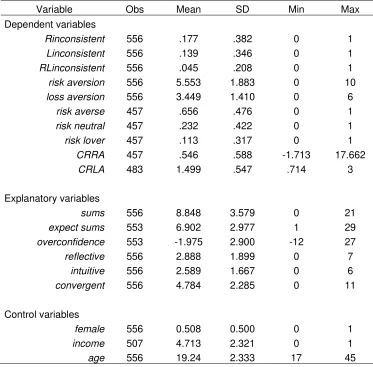
Table 1 displays descriptive statistics for all the dependent and explanatory variables used. As can be seen, the sample is reduced in three observations
for expect sums and hence for overconfidence due to the exclusion of outliers
[image:13.595.109.482.330.697.2](using the mean ± 3 SD rule).
Table 1. Descriptive statistics (computed using sampling weights)
Variable Obs Mean SD Min Max
Dependent variables
Rinconsistent 556 .177 .382 0 1 Linconsistent 556 .139 .346 0 1 RLinconsistent 556 .045 .208 0 1 risk aversion 556 5.553 1.883 0 10 loss aversion 556 3.449 1.410 0 6
risk averse 457 .656 .476 0 1 risk neutral 457 .232 .422 0 1 risk lover 457 .113 .317 0 1
CRRA 457 .546 .588 -1.713 17.662 CRLA 483 1.499 .547 .714 3
Explanatory variables
sums 556 8.848 3.579 0 21
expect sums 553 6.902 2.977 1 29 overconfidence 553 -1.975 2.900 -12 27 reflective 556 2.888 1.899 0 7
intuitive 556 2.589 1.667 0 6 convergent 556 4.784 2.285 0 11
Control variables
female 556 0.508 0.500 0 1 income 507 4.713 2.321 0 1
age 556 19.24 2.333 17 45
In addition, all the dependent variables that require parameterization, i.e., risk
whose decisions are consistent throughout the task since these measures cannot be computed for inconsistent decisions. This involves excluding 99 observations in the former four cases and 73 observations in the latter case (see Rinconsistent and Linconsistent in Table 1).
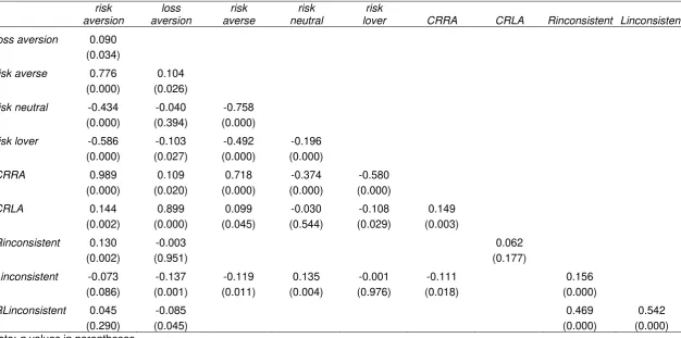
Tables 2 and 3 show zero-order Pearson correlations between the DMU (and inconsistent DMU) and CAbs variables, respectively. The impact of CAbs on DMU will be studied below using regression analysis. Regarding the relationships between our dependent variables, we observe that the number of risk averse and loss averse choices, that is, risk aversion and loss
aversion, are positively albeit weakly correlated (p = 0.03), as expected. This
correlation becomes stronger when using the parametric measures of risk and loss aversion, CRRA and CRLA, which exclude inconsistent individuals
(p < 0.01). Also, a larger number of risk averse choices is positively
associated with being inconsistent in the risk aversion task (Rinconsistent;
p < 0.01) and negatively, but marginally, associated with being inconsistent in
the loss aversion task (Linconsistent; p = 0.09). These results translate into
relationships in the expected direction, which are sometimes significant when the risk dummies (risk averse, risk neutral and risk loving) are considered. On
the other hand, a larger number of loss averse choices is negatively associated with Linconsistent (p < 0.01). Finally, Rinconsistent and
Linconsistent are positively related (p < 0.01).
These results are important because they reflect the fact that being inconsistent is linked to a larger number of risk averse choices and a smaller number of loss averse choices.
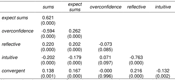
For the explanatory variables, Table 3 shows that math proficiency (sums) is
strongly positively correlated with individuals’ expectations (expect sums), but
negatively with overconfidence (both p < 0.01). As expected, sums are
positively correlated with both reflective and, to a lesser extent, convergent,
and negatively correlated with intuitive (all p < 0.01). Similar relationships are
observed for expect sums (all p < 0.01). Overconfidence is negatively
(positively) related to reflective (intuitive), although both relationships are
marginal (both about p = 0.09). Finally, reflective (intuitive) is positively
Table 2. Zero-order Pearson correlations for DMU and inconsistent DMU variables (computed using sampling weights)
risk aversion
loss aversion
risk averse
risk neutral
risk
lover CRRA CRLA Rinconsistent Linconsistent
loss aversion 0.090 (0.034)
risk averse 0.776 0.104 (0.000) (0.026)
risk neutral -0.434 -0.040 -0.758 (0.000) (0.394) (0.000)
risk lover -0.586 -0.103 -0.492 -0.196 (0.000) (0.027) (0.000) (0.000)
CRRA 0.989 0.109 0.718 -0.374 -0.580 (0.000) (0.020) (0.000) (0.000) (0.000)
CRLA 0.144 0.899 0.099 -0.030 -0.108 0.149 (0.002) (0.000) (0.045) (0.544) (0.029) (0.003)
Rinconsistent 0.130 -0.003 0.062
(0.002) (0.951) (0.177)
Linconsistent -0.073 -0.137 -0.119 0.135 -0.001 -0.111 0.156 (0.086) (0.001) (0.011) (0.004) (0.976) (0.018) (0.000)
RLinconsistent 0.045 -0.085 0.469 0.542
(0.290) (0.045) (0.000) (0.000)
Table 3. Zero-order Pearson correlations for CAbs variables
sums expect
sums overconfidence reflective intuitive
expect sums 0.621 (0.000)
overconfidence -0.594 0.262 (0.000) (0.000)
reflective 0.220 0.202 -0.073 (0.000) (0.000) (0.085)
intuitive -0.202 -0.179 0.071 -0.763 (0.000) (0.000) (0.097) (0.000)
convergent 0.138 0.167 -0.000 0.216 -0.132 (0.001) (0.000) (0.996) (0.000) (0.002) Note: p-values in parentheses. Correlations computed using sampling weights.
III-b The impact of CAbs on inconsistent choices
Before analyzing the relationship between the CAbs measures and the risk preferences measures, we explore the impact of CAbs on inconsistent choices. We have six explanatory variables and three dependent variables. This means that we have 18 models to test.
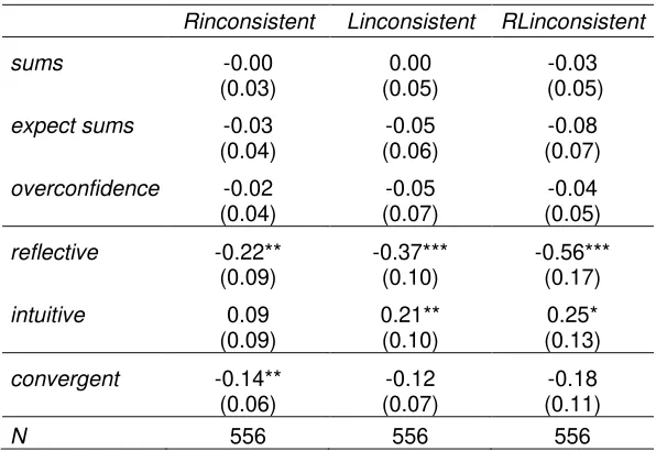
Table 4 shows the estimated impact of our set of CAbs on inconsistent DMU using logit regression models. Each column focuses on a particular measurement of inconsistency, whereas rows refer to the different CAbs measures (each cell shows estimates obtained from a different model; the constant is not shown). We use sampling weights in all regressions.
We find that more reflective individuals are less likely to make inconsistent
choices in both tasks (Rinconsistent, p = 0.01, Linconsistent and
RLinconsistent, p < 0.01; the opposite is observed for intuitive, but only
significant for Linconsistent, p = 0.04 and RLinconsistent, p = 0.05). The
individuals displaying better convergent thinking are also less likely to make
inconsistent choices in the risk aversion task (p = 0.02; not significant for
Linconsistent, p = 0.12 or RLinconsistent, p = 0.10).
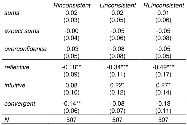
All the regressions are replicated controlling for gender, age and income in Table A.1 of Appendix 1.12 The results remain qualitatively unchanged.
Table 4. The impact of CAbs on inconsistent DMU
Rinconsistent Linconsistent RLinconsistent
sums -0.00 0.00 -0.03
(0.03) (0.05) (0.05) expect sums -0.03 -0.05 -0.08
(0.04) (0.06) (0.07) overconfidence -0.02 -0.05 -0.04 (0.04) (0.07) (0.05) reflective -0.22** -0.37*** -0.56***
(0.09) (0.10) (0.17) intuitive 0.09 0.21** 0.25* (0.09) (0.10) (0.13) convergent -0.14** -0.12 -0.18 (0.06) (0.07) (0.11)
N 556 556 556
Notes: Each cell corresponds to a different regression. Robust standard errors in parentheses. Regressions using expect sums or overconfidence also exclude the three outliers detected. Sampling weights are enabled in all regressions. *** p < 0.01, ** p < 0.05, * p < 0.10.
A second robustness check is implemented in Table A.2 (Appendix 1) in which the main explanatory variables (i.e., sums, expect sums, reflective and
convergent) are all included together (since overconfidence is determined by
sums and expect sums, we only enable reflective for the CRT since also
including intuitive would yield collinearity).
From this analysis, we observe that both reflective and convergent remain
significant or marginally significant in predicting inconsistent risk choices
(Rinconsistent) when included together, which means that they operate
independently to some extent. Reflective is still also significant in predicting
inconsistent choices in the loss aversion task and in both tasks together. Adding controls does not substantially change the results (not reported).
model is lower than for the linear model. Taking into account the above conditions, quadratic models are better than their linear counterparts in the following cases: Rinconsistent explained by sums, Linconsistent explained by
overconfidence and Rinconsistent explained by overconfidence (see
Appendix 2 for details).
In sum, our data show that subjects who score high in the CRT and the RAT are less likely to be inconsistent. The latter implies that restricting the sample to participants who make consistent MPL choices implies selecting those
endowed with better cognitive abilities.
III-c The impact of CAbs on DMU
Finally, we explore the impact of the different CAbs measures on our DMU dependent variables. In this case we have six explanatory variables and seven dependent variables. This means that we have 42 models to test.
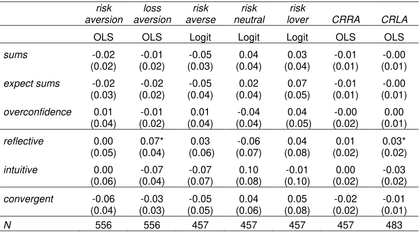
Table 5 shows the estimated impact of our set of CAbs on DMU using regression models. As in Table 4, each column focuses on a particular measurement of DMU, whereas rows refer to the different CAbs measures (each cell shows estimates obtained from a different model; the constant is not shown). OLS estimations are used for the continuous dependent variables and logit for the binary ones. We use sampling weights in all regressions.
The results are quite straightforward. We do not find any robust link between our cognitive measures and DMU. We only observe a marginally positive effect of reflective on loss aversion (p = 0.09) and CRLA (p = 0.06). Thus,
more analytic individuals are more loss averse, in line with previous studies (see Dohmen et al. 2018), albeit the relationship is rather weak.
A second robustness check is implemented in Table A.4 in which the main explanatory variables (i.e., sums, expect sums, reflective and convergent) are
included together (see above). From this analysis, we observe that the marginally significant positive effects of reflective on loss aversion and CRLA
loving. Adding controls does not substantially change the results (not
reported).
The models reported in Table 5 were repeated including the squared term of the explanatory variables. Using the same three conditions as above, we find that the quadratic model is better than linear model for risk averse and risk
neutral, as explained by sums. The coefficients associated to sums and sums
squared are, respectively, 0.13 (p = 0.20) and -0.01 (p = 0.06) for risk neutral
and -0.17 (p = 0.13) and 0.01 (p = 0.03) for risk averse. In both cases,
[image:20.595.90.507.315.548.2]however, the power of fit of the quadratic model is rather poor and the joint significance test only yields marginal significance.
Table 5. The impact of CAbs on DMU
risk
aversion aversion loss averse risk neutral risk lover risk CRRA CRLA OLS OLS Logit Logit Logit OLS OLS sums -0.02 -0.01 -0.05 0.04 0.03 -0.01 -0.00 (0.02) (0.02) (0.03) (0.04) (0.04) (0.01) (0.01) expect sums -0.02 -0.02 -0.05 0.02 0.07 -0.01 -0.00 (0.03) (0.02) (0.04) (0.04) (0.05) (0.01) (0.01) overconfidence 0.01 -0.01 0.01 -0.04 0.04 -0.00 0.00
(0.04) (0.02) (0.04) (0.04) (0.05) (0.02) (0.01) reflective 0.00 0.07* 0.03 -0.06 0.04 0.01 0.03* (0.05) (0.04) (0.06) (0.07) (0.08) (0.02) (0.02) intuitive 0.00 -0.07 -0.07 0.10 -0.01 0.00 -0.03 (0.06) (0.04) (0.07) (0.08) (0.10) (0.02) (0.02) convergent -0.06 -0.03 -0.05 0.04 0.05 -0.02 -0.01 (0.04) (0.03) (0.05) (0.06) (0.08) (0.02) (0.01)
N 556 556 457 457 457 457 483
Notes: Each cell corresponds to a different regression. Robust standard errors in parentheses. The differences in sample sizes across regressions stem from the fact that, except for non-parametric measures such as risk aversion and loss aversion, values cannot be calculated for individuals with inconsistent choices and are therefore excluded. The regressions using expect sums or overconfidence also exclude the three outliers detected. Sampling weights are enabled in all regressions. *** p < 0.01, ** p < 0.05, * p < 0.10.
All the regressions are replicated controlling for gender, age and income in Table A.3 in the Appendix. The results remain qualitatively unchanged, except for a marginal negative (positive) relationship between expect sums and loss
aversion (risk loving). Moreover, the effect of reflective on loss aversion loses
All in all, our results show that there is not a robust link between our measures of cognitive abilities and DMU.
V Conclusions
Using a large, nationally representative sample of participants comprising Business Economics students, our study yields two important results.
First, the study supports the hypothesis that risk preferences are not correlated to individuals’ math proficiency, analytical (reflective) thinking or convergent thinking.
Second, we find that individuals who rely more on reflection than intuition and those displaying better convergent thinking are less likely to make inconsistent choices in the risk-related tasks.
Therefore, our results indicate that preferences for risk in either the gain or the
loss domain are not driven by cognitive abilities. Although we find weak
evidence that more analytical/reflective individuals are more loss averse (in line with previous literature; see Dohmen et al. 2018), taken together, our results instead support the notion that low CAbs are related to noisy, inconsistent decision making. This result is particularly salient when CAbs are measured as analytical/reflective (vs. intuitive) thinking and, to a lesser extent, as convergent thinking.
An important contribution of this paper is related to selection. If subjects who fail to pass the consistency requirement are dropped from the sample and these subjects are those with lower cognitive abilities, then the restricted
sample selects participants who have higher cognitive abilities. Since being
Still there is a more intricate problem related to the potential number of individuals whose choices are labeled as consistent by chance. This is the case, for instance, of subjects who never switch (which might be related to inattention) or those who make consistent choices by chance although they do not understand the decisions. Detecting these individuals does not seem to be an easy endeavor. A potential solution might be to ask subjects about the procedure they follow to make the choices.
References
Åkerlund, D., Golsteyn, B.H., Grönqvist, H. andLindahl, L. (2016). Time discounting and criminal behavior. Proceedings of the National Academy of
Sciences 113(22): 6160–6165.
https://doi.org/10.1073/pnas.1522445113
Anderhub, V., Müller, R. and Schmidt, C. (2001). Design and evaluation of an economic experiment via the Internet. Journal of Economic Behavior &
Organization 46(2): 227–247.
https://doi.org/10.1016/S0167-2681(01)00195-0
Andersson, O., Holm, H. J., Tyran, J. R. andWengström, E. (2016).Risk Aversion Relates to Cognitive Ability: Preferences or Noise? Journal of the
European Economic Association 14(5): 1129–1154.
https://doi.org/10.1111/jeea.12179
Angrisani M. and Casanova, M.(2011). Understanding Heterogeneity in Household Portfolios: The Role of Cognitive Ability and Preference Parameters. Mimeo USC.
Angrisani M. and Casanova, M. (2018). Portfolio Allocations of Older Americans: The Role of Cognitive Ability and Preference Parameters. Mimeo
USC.
Arechar, A. A., Gächter, S. and Molleman, L. (2018). Conducting interactive experiments online. Experimental Economics 21(1): 99–131.
https://doi.org/10.1007/s10683-017-9527-2
Beauchamp, J. P., Benjamin, D. J. and Chabris, C. F. (2012). How Malleable are Risk Preferences and Loss Aversion? Mimeo USC.
Beauchamp, J. P.,·Cesarini, D. and·Johannesson, M. (2017). The psychometric and empirical properties of measures of risk preferences.
Journal of Risk and Uncertainty 54(3): 203–237.
https://doi.org/10.1007/s11166-017-9261-3
Benjamin, D. J., Brown, S. A. and Shapiro, J. M. (2013).Who is Behavioral? Cognitive Ability and Anomalous Preferences. Journal of the European
Economic Association 11(6): 1231–1255.
https://doi.org/10.1111/jeea.12055
Berns, G. S., Capra, C. M., Chappelow, J., Moore, S., Noussair, C. (2008). Nonlinear neurobiological probability weighting functions for aversive outcomes, Neuroimage 39(4): 2047–2057.
https://dx.doi.org/10.1016%2Fj.neuroimage.2007.10.028
Bickel, W. K., Odum, A. L. and Madden, G. J. (1999). Impulsivity and cigarette smoking: delay discounting in current, never, and ex-smokers.
Booth, A. I. and Katic, P. (2013). Cognitive Skills, Gender and Risk Preferences. Economic Record 89(284): 19–30.
https://doi.org/10.1111/1475-4932.12014
Booth, A., Cardona-Sosa, L. and Nolen, P. (2014). Gender Differences in Risk Aversion: Do Single-Sex Environments Affect Their Development? Journal of
Economic Behavior & Organization 99: 126–54.
https://doi.org/10.1016/j.jebo.2013.12.017
Bosch-Domènech, A., Brañas-Garza, P. and Espín, A. M. (2014). Can exposure to prenatal sex hormones (2D: 4D) predict cognitive reflection?
Psychoneuroendocrinology 43: 1–10.
https://doi.org/10.1016/j.psyneuen.2014.01.023
Brañas-Garza, P., Guillen, P., Lopez, R. (2008). Math skills and risk attitudes.
Economics Letters 99(2): 332–36.
https://doi.org/10.1016/j.econlet.2007.08.008
Brañas-Garza, P., and Rustichini A. (2011). Organizing effects of testosterone and economic behavior: Not just risk taking. PLoS ONE 6(12): e29842.
https://doi.org/10.1371/journal.pone.0029842
Brañas-Garza, P., Kujal, P. and Lenkei, B. (2015). Cognitive Reflection Test: Whom, how, when. Munich Repository 68049.
Burks, S. V., Carpenter, J. P., Goette, L. and Rustichini, A. (2009). Cognitive Skills Affect Economic Preferences, Strategic Behavior, and Job Attachment.
Proceedings of the National Academy of Sciences106(19): 7745–50.
https://doi.org/10.1073/pnas.0812360106
Campitelli, G. and Labollita, M. (2010). Correlations of cognitive reflection with judgments and choices. Judgment and Decision Making 5(3): 182–91.
Capraro, V., Corgnet, B., Espín, A. M. and Hernán-González, R. (2017). Deliberation favours social efficiency by making people disregard their relative shares: evidence from USA and India. Royal Society Open Science 4(2):
160605.
https://dx.doi.org/10.1098%2Frsos.160605
Chapman, J.,Snowberg, E., Wang, S. and Camerer. C. (2018). Loss Attitudes in the U.S. Population: Evidence from Dynamically Optimized Sequential Experimentation (DOSE). NBER Working Paper 25072.
Charness, G., Gneezy, U. and Imas, A. (2013). Experimental methods: Eliciting risk preferences. Journal of Economic Behavior & Organization 87:
43–51.
Charness, G., Gneezy, U., and Halladay, B. (2016). Experimental methods: Pay one or pay all. Journal of Economic Behavior & Organization 131(Part A):
141–150.
https://doi.org/10.1016/j.jebo.2016.08.010
Christelis, D., Jappelli, T. and Padula, M. (2010). Cognitive Abilities and Portfolio Choice. European Economic Review 54(1):18–38.
https://doi.org/10.1016/j.euroecorev.2009.04.001
Cokely, E. T. and Kelley, C. M. (2009). Cognitive abilities and superior decision making under risk: A protocol analysis and process model evaluation. Judgment and Decision Making 4(1): 20–33.
Cole, S., Paulson, A. and Shastry, G. K. (2014). Smart Money? The Effect of Education on Financial Outcomes. The Review of Financial Studies 27(7):
2022–2051.
https://doi.org/10.1093/rfs/hhu012
Corgnet, B., Espín, A. M. and Hernán-González, R. (2016). Creativity and cognitive skills among millennials: thinking too much and creating too little.
Frontiers in psychology 7: 1626.
https://doi.org/10.3389/fpsyg.2016.01626
Cueva, C., Iturbe-Ormaetxe, I., Mata-Pérez, E., Ponti, G., Sartarelli, M., Yu,H. and Zhukova, V. (2015). Cognitive (ir)reflection: New experimental evidence.
Journal of Behavioral & Experimental Economics 64: 81–93.
https://doi.org/10.1016/j.socec.2015.09.002
Dohmen, T., Falk, A., Huffman, D. and Sunde, U. (2010). Are Risk Aversion and Impatience Related to Cognitive Ability? The American Economic Review
100(3): 1238–1260.
Dohmen, T., Falk, A., Huffman, D. and Sunde, U. (2018).On the Relationship between Cognitive Ability and Risk Preference. Journal of Economic
Perspectives 32(2): 115–134.
https://doi.org/10.1257/jep.32.2.115
Eckel, C. C. and Grossman, P. J. (2002). Sex differences and statistical stereotyping in attitudes toward financial risk. Evolution and Human Behavior,
23(4): 281–295.
https://doi.org/10.1016/S1090-5138(02)00097-1
Falk, A., Becker, A., Dohmen, T., Enke, B., Huffman, D. and Sunde, U. (2018). Global Evidence on Economic Preferences. The Quarterly Journal of
Economics 133(4): 1645–1692.
https://doi.org/10.1093/qje/qjy013
Frederick, S. (2005). Cognitive Reflection and Decision Making. Journal of
Economic Perspectives 19(4): 25–42.
Frisell, T., Pawitan, Y. and Långström, N. (2012). Is the Association Between General Cognitive Ability and Violent Crime Caused by Family-Level Confounders? PloS ONE 7(7): e41783.
https://doi.org/10.1371/journal.pone.0041783
Gächter, S., Johnson, E. J. and Herrmann, A. (2007). Individual-level loss aversion in riskless and risky choices. IZA Discussion Paper 2961.
Grinblatt, M., Keloharju, M. and Linnainmaa, J.(2011). IQ and Stock Market Participation. The Journal of Finance 66(6): 2121–64.
Holt, C. A. and Laury, S. K. (2002). Risk Aversion and Incentive Effects. The
American Economic Review92(5): 1644–1655.
Horton, J. J., Rand, D. G. and Zeckhauser, R. J. (2011). The online laboratory: Conducting experiments in a real labor market. Experimental
Economics 14(3): 399–425.
https://doi.org/10.1007/s10683-011-9273-9
Lilleholt, L. (2019). Cognitive ability and risk aversion: A systematic review and meta analysis. Judgment and Decision Making 14(3): 234–279.
Mandal, B. and Roe, B. E. (2014). Risk tolerance among National Longitudinal Survey of Youth participants: The effects of age and cognitive skills.
Economica, 81(323): 522–543.
https://doi.org/10.1111/ecca.12088
Mather, M., Mazar, N., Gorlick, M. A., Lighthall, N. R., Burgeno, J., Schoeke, A. and Ariely, D. (2012). Risk Preferences and Aging: The “Certainty Effect” in Older Adults´ Decision Making. Psychology and Aging 27(4): 801–16.
https://doi.org/10.1037/a0030174
Mednick, S. A. (1962). The associative basis of the creative process.
Psychological Review 69(3): 220–32.
https://psycnet.apa.org/doi/10.1037/h0048850.
Meier, S. and Sprenger, C. D. (2012). Time discounting predicts creditworthiness. Psychological Science 23(1): 56–58.
https://doi.org/10.1177%2F0956797611425931
Niederle, M. and Vesterlund, L. (2007). Do women shy away from competition? Do men compete too much? The Quarterly Journal of
Economics 122(3): 1067–1101.
https://doi.org/10.1162/qjec.122.3.1067
Oechssler, J., Roider, A. and Schmitz, P. W. (2009). Cognitive abilities and behavioral biases. Journal of Economic Behavior and Organization 72(1):
147–52.
Pachur, T., Mata, R. and Hertwig, R. (2017). Who Dares, Who Errs? Disentangling Cognitive and Motivational Roots of Age Differences in Decisions Under Risk. Psychological Science 28(4): 504–518.
https://doi.org/10.1177%2F0956797616687729
Park, N. Y. (2016). Domain-specific risk preference and cognitive ability.
Economics Letters 141: 1–4.
https://doi.org/10.1016/j.econlet.2016.01.008
Rustichini, A., DeYoung, C. G., Anderson, J. and Burks, S. V. (2016). Toward the Integration of Personality Theory and Decision Theory in Explaining Economic Behavior: An Experimental Investigation. Journal of Behavioral &
Experimental Economics 64: 122-37.
https://doi.org/10.1016/j.socec.2016.04.019
Shen, W., Hommel, B., Yuan, Y., Chang, L. and Zhang, W. (2018). Risk-taking and creativity: Convergent, but not divergent thinking is better in low-risk takers. Creativity Research Journal 30(2): 224–231.
https://doi.org/10.1080/10400419.2018.1446852
Sousa, S. (2010). Are Smarter People Really Less Risk Averse? CeDEx
Discussion Paper Series 2010-17.
Sutter, M., Kocher, M. G., Glätzle-Rützler, D. and Trautmann, S. T. (2013). Impatience and Uncertainty: Experimental Decisions Predict Adolescents' Field Behavior. The American Economic Review 103(1): 510–531.
http://dx.doi.org/10.1257/aer.103.1.510
Taylor, M. P. (2013). Bias and brains: Risk aversion and cognitive ability across real and hypothetical settings. Journal of Risk and Uncertainty 46(3):
299–320.
https://doi.org/10.1007/s11166-013-9166-8
Taylor, M. P. (2016). Are High-Ability Individuals Really More Tolerant of Risk? A Test of the Relationship Between Risk Aversion and Cognitive Ability.
Journal of Behavioral and Experimental Economics 63: 136–147.
https://doi.org/10.1016/j.socec.2016.06.001
Toplak, M. E., West, R. F. and Stanovich, K. E. (2014). Assessing miserly information processing: An expansion of the Cognitive Reflection Test.
Thinking and Reasoning 20(2): 147–168.
https://doi.org/10.1080/13546783.2013.844729
Tymula, A., Rosenberg-Belmaker, L. A., Roy, A. K., Ruderman, L., Manson, K., Glimcher, P. W. and Levy, I. (2012). Adolescents' risk-taking behavior is driven by tolerance to ambiguity. Proceedings of the National Academy of
Sciences, 109(42): 17135–17140.
Van Rooij, M., Lusardi, A. and Alessie, R. (2011). Financial Literacy and Stock Market Participation. Journal of Financial Economics 101(2): 449–472.
APPENDIX 1: Additional regressions
Table A.1. Regression analysis with controls. The impact of CAbs on
inconsistent DMU
Rinconsistent Linconsistent RLinconsistent
sums 0.02
(0.03) (0.05) 0.02 (0.06) 0.01 expect sums -0.00
(0.04)
-0.05 (0.06)
-0.05 (0.08) overconfidence -0.03
(0.05) (0.08) -0.08 (0.05) -0.05 reflective -0.18**
(0.09) -0.34*** (0.11) -0.49*** (0.17) intuitive 0.08
(0.10) (0.12) 0.22* (0.14) 0.27* convergent -0.14**
(0.06) (0.07) -0.08 (0.11) -0.13
N 507 507 507
Notes: Each cell corresponds to a different regression. Robust standard errors in parentheses. The regressions using expect sums or overconfidence also exclude the three outliers detected. Sampling weights are enabled in all regressions. *** p < 0.01, ** p < 0.05, * p < 0.10.
Table A.2. Regression analysis with all explanatory variables simultaneously.
The impact of CAbs on inconsistent DMU
Rinconsistent Linconsistent RLinconsistent
sums 0.03 0.07 0.05
(0.04) (0.06) (0.05) expect sums -0.01 -0.04 -0.04
(0.06) (0.09) (0.09) reflective -0.20** -0.36*** -0.54***
(0.09) (0.10) (0.20) convergent -0.11* -0.06 -0.10
(0.06) (0.07) (0.11)
N 553 553 553
[image:29.595.144.453.446.592.2]Table A.3. Regression analysis with controls. The impact of CAbs on DMU risk aversion loss aversion risk averse risk neutral risk
lover CRRA CRLA OLS OLS Logit Logit Logit OLS OLS
sums -0.02
(0.02) (0.02) -0.01 (0.03) -0.04 (0.04) 0.03 (0.04) 0.04 (0.01) -0.01 (0.01) -0.01 expect sums -0.01
(0.04) -0.04* (0.02) (0.04) -0.04 (0.05) -0.00 (0.04) 0.08* (0.01) -0.01 (0.01) -0.01 overconfidence 0.02
(0.04) (0.03) -0.02 (0.04) 0.01 (0.05) -0.04 (0.05) 0.03 (0.02) 0.00 (0.01) 0.00 reflective 0.04
(0.05) 0.07 (0.04) 0.08 (0.07) -0.09 (0.08) -0.02 (0.09) 0.02 (0.02) 0.03* (0.02) intuitive -0.02
(0.06) (0.05) -0.07 (0.08) -0.12 (0.09) 0.10 (0.09) 0.08 (0.02) -0.01 (0.02) -0.03 convergent -0.06
(0.05) (0.03) -0.05 (0.06) -0.06 (0.06) 0.04 (0.09) 0.07 (0.02) -0.02 (0.01) -0.01
N 507 507 417 417 417 417 440
Table A.4. Regression analysis with all explanatory variables simultaneously. The
impact of CAbs on DMU
risk
aversion aversion loss averse risk neutral risk lover risk CRRA CRLA
OLS OLS Logit Logit Logit OLS OLS
sums -0.01 -0.00 -0.03 0.05 -0.02 -0.00 -0.01 (0.04) (0.02) (0.04) (0.04) (0.05) (0.01) (0.01) expect sums -0.00 -0.02 -0.03 -0.01 0.08* -0.01 -0.00
(0.05) (0.03) (0.04) (0.05) (0.05) (0.02) (0.01) reflective 0.02 0.09** 0.06 -0.08 0.03 0.01 0.04** (0.05) (0.04) (0.06) (0.07) (0.09) (0.02) (0.02) convergent -0.06 -0.04 -0.05 0.05 0.03 -0.02 -0.01
(0.05) (0.03) (0.05) (0.06) (0.09) (0.02) (0.01)
[image:30.595.91.505.377.550.2]APPENDIX 2: Quadratic models for Inconsistency
As explained throughout the paper, we can say that the quadratic model is better than the linear model if three conditions are verified: the quadratic term is significant, the linear and quadratic terms are jointly significant and the Bayesian information criterion for the quadratic model is lower than for the linear model.
Only three models verify the three conditions:
• Rinconsistent explained by sums. The coefficients associated to sums
and sums squared are, respectively, 0.32 (p = 0.02) and -0.02
(p = 0.01). This means that individuals with about eight correct sums
are the most likely to make inconsistent choices in the risk aversion task. Individuals with more or less than eight correct answers were less likely to make inconsistent choices. A possible explanation is the lack of motivation: those with less than eight correct answers do not really care about this task or find it too tiresome (note that for BusEc students, having at least eight correct answers in 60 seconds should be very easy), hence low math proficiency should not be the determinant of extremely low values of sums. If this is the case, this
result would be indicating that math proficiency is also (just as
reflective and convergent) negatively related to inconsistent risk
choices.
• Linconsistent explained by overconfidence. The coefficients associated
to overconfidence and its square are, respectively, -0.50 (p = 0.22) and
0.01 (p = 0.01). However, this result is uniquely due to two individuals
with overconfidence higher than 10 (i.e., they expected > 10 correct
answers more than they actually had). In excluding these two observations, the significance completely vanishes.
• RLinconsistent explained by overconfidence. The coefficients
associated to overconfidence and its square are, respectively, -0.40
(p = 0.11) and -0.08 (p = 0.03). Yet, again, this result vanishes after
APPENDIX 3: Instructions for risk and loss aversion tasks Risk aversion:
You are now going to make 10 decisions about a certain amount of money associated with different probabilities. In each scenario you will have to choose between two lotteries that assign a probability to two possible monetary gains (prizes). Note that choosing a lottery implies playing it.
The 10 decisions are totally independent of each other. There are no right or wrong answers. Make the decision that you feel matches with your own preferences. Do not take into account what you decided previously or will decide later.
Payment: For real payments we will randomly select 1 out of 10 decisions. Then you will play the lottery you chose in that scenario. So, think carefully about your decisions because this will determine the amount of money you will earn (if you are selected).
Please, press START to begin the task
Start
Choose between the two options for each decision, the one you prefer
1. €€40 with 10% probability 32 with 90% probability €€77 with 10% probability 2 with 90% probability
2. €€40 with 20% probability 32 with 80% probability €€77 with 20% probability 2 with 80% probability
3. €€40 with 30% probability 32 with 70% probability €€77 with 30% probability 2 with 70% probability
4. €€40 with 40% probability 32 with 60% probability €€77 with 40% probability 2 with 60% probability
5. €€40 with 50% probability 32 with 50% probability €€77 with 50% probability 2 with 50% probability
6. €€40 with 60% probability 32 with 40% probability €€77 with 60% probability 2 with 40% probability
7. €€40 with 70% probability 32 with 30% probability €€77 with 70% probability 2 with 30% probability
8. €€40 with 80% probability 32 with 20% probability €€77 with 80% probability 2 with 20% probability
9. €€40 with 90% probability 32 with 10% probability €€77 with 90% probability 2 with 10% probability
Loss aversion:
Just for starting you will receive a €35 endowment. During this task you will have to make 6 decisions about negative (losses) or positive (gains) amounts
of money. In each decision you will be asked to accept or refuse to play a lottery. The lottery is extremely simple: we flip a virtual coin and if it comes up heads, you can win money, otherwise you lose. The lottery is always the same, but from scenario to scenario the amount you lose increases. Note that choosing a lottery implies playing it (you may either win or lose).
The 6 decisions are totally independent of each other. There are no right or wrong answers. Make the decision that you feel matches with your own preferences. Do not take into account what you decided previously or will decide later.
The amount of money you earn here by playing the lottery will be added to the initial endowment of €35.
Payment: One of your 6 decisions will be chosen randomly for real payments. Then we will check whether you decided to play the lottery or not. If you did, we will toss the coin to determine whether you earn or lose the prize. If you have refused to play, then you will earn €0 plus €35. The €35 endowment is to cover potential losses.
Please press START to begin the task
Start
For each decision, choose if you accept or reject playing the lottery. If you reject it, you do not gain or lose anything.
1. If it's tails, you lose €10 and if it's heads you win €30 Accept Reject
2. If it's tails, you lose €15 and if it's heads you win €30 Accept Reject
3. If it's tails, you lose €20 and if it's heads you win €30 Accept Reject
4. If it's tails, you lose €25 and if it's heads you win €30 Accept Reject
5. If it's tails, you lose €30 and if it's heads you win €30 Accept Reject