On the effects of static and autoregressive conditional higher order moments on dynamic optimal hedging

Munich Personal RePEc Archive

On the effects of static and

autoregressive conditional higher order

moments on dynamic optimal hedging

Hou, Yang and Holmes, Mark

School of Accounting, Economics and Finance Waikato Management

School University of Waikato, School of Accounting, Economics and

Finance Waikato Management School University of Waikato

17 October 2017

Online at

https://mpra.ub.uni-muenchen.de/82000/

On the effects of static and autoregressive conditional higher order

moments on dynamic optimal hedging

Yang (Greg) Hou

School of Accounting, Economics and Finance

Waikato Management School

University of Waikato

Private Bag 3105, Hamilton, 3240, New Zealand

Email-address: [email protected]

Telephone number: +64-7-8379402

and

Mark Holmes*

School of Accounting, Economics and Finance

Waikato Management School

University of Waikato

Private Bag 3105, Hamilton, 3240, New Zealand

Email-address: [email protected]

2

On the effects of static and autoregressive conditional higher order

moments on dynamic optimal hedging

Abstract

While dynamic optimal hedging is of major interest, it remains unclear as to whether incorporating higher moments of a return distribution leads to better hedging decisions. We examine the effects of introducing a bivariate skew-Student density function with static and autoregressive conditional skewness and kurtosis on dynamic minimum-variance hedging strategies. Static higher order moments improve reductions in variance and value at risk of hedged portfolios. The inclusion of dynamics through an autoregressive component extends these improvements further. These benefits avail for short and long hedging horizons, which is highlighted in the global financial crisis. The static and conditional higher order moments enhance the notion that the size and smoothness of hedge ratios positively relate to hedging effectiveness while volatility does the reverse. Improved effectiveness can be explained given an upgrade of size and smoothness and a downgrade of volatility of hedge ratios attributed to the dynamics of higher order moments.

1

The effects of static and autoregressive conditional higher order moments

on dynamic optimal hedging

1. Introduction

A departure from the normality of financial return distributions is widely acknowledged in

the literature, see for example Harvey (1995), Agarwal and Naik (2004), Brooks and Kat

(2002), Harvey and Siddique (2000), and Christie-David and Chaudhry (2001), among others.

Investors exhibit a preference for information on higher order moments, other than the mean

and variance of asset returns (Scott and Horvarth, 1980; Brook et al., 2012). Such a

preference is incorporated via pricing of systematic risk related to skewness (Kraus and

Litzenberger, 1976, 1983; Harvey and Siddique, 2000)1 and optimal asset allocation impacted

by kurtosis (Kallberg and Ziemba, 1983; Jondeau and Rockinger, 2006). A consensus has

almost been reached insofar as ignoring the effects of higher order moments on asset pricing

and portfolio management may lead to sub-optimal investment decisions (Brook et al., 2012).

The effect of higher order moments above the variance on hedging decisions has drawn

attention in the recent finance literature. The conventional determination of the optimal hedge

ratio (OHR), which is the optimal amount of futures contracts to employ per unit of the cash

asset to be hedged (Ederington, 1979), assumes that investors have a two-moment utility

function or that the distribution of asset returns is normal. Such an assumption is criticised

since return distributions are not normal and investors have additional aversions to negative

skewness and positive excess kurtosis (Levy 1969; Brooks et al., 2012). Hence hedging

strategies ignoring these facts might lead to sub-optimal hedging decisions (Brooks et al.,

2012).

1 _{Attempts on the incorporation of skewness are also made with respect to investment decisions (Hong et al.,}

2

There is a small group of studies that incorporate the impact of higher order moments

into the optimal hedging. The focus thus far has been on minimum variance or maximum

utility hedging strategies that generate static OHRs. The effects of skewness and kurtosis of

returns of the hedged portfolio with volatility minimised have been taken into account by

Harris and Shen (2006) and Cao et al. (2009) where the OHRs comprising the hedged

portfolio are derived by a minimisation of value at risk (VaR) and conditional VaR (CVaR)

of the hedged portfolio. The effect of the third moment is addressed in minimum variance

hedging by Lien and Shrestha (2010) with a skew-normal distribution and Fu (2014) with a

multi-objective hedging model. In addition to this, Gilbert et al. (2006) focuses on a partial

equilibrium model allowing for skewness only in the hedger’s utility function to determine

OHRs. Brook et al. (2012) propose a more generalised utility-based framework that accounts

for all the moments of return distribution. The general message from these studies is that

using information based on moments higher than the variance lead to the better hedging

decisions involving the use of static OHRs.

A drawback associated with the static hedging strategy that it leads to sub-optimal

decisions in periods of high basis volatility. The reason is that the derivation of the static

OHRs ignores the dynamics between the cash and futures returns that are conditional on the

past information set. Hence one intuitively expects the OHRs to be time varying, which has

been extensively modelled for the minimum-variance hedging strategies by the multivariate

generalised autoregressive conditionally heteroscedastic (MGARCH) family of models (see,

e.g. Kroner and Sultan, 1993; Bera et al., 1997; Brooks et al., 2002; Baillie et al., 2007; Park

and Jei, 2010; Park and Kim, 2016). The derivation of the conditional OHRs substantially

depends on the multivariate probability density functions (PDF) of return distributions, the

logarithmic likelihood of which is maximised to obtain estimates of the MGARCH model. A

3

related to the dynamic optimal hedging since the multivariate return distributions are

non-normal (Engle and Gonzalez-Rivera, 1991; Bollerslev, 1987; Baillie and Bollerslev, 1989;

Susmel and Engle, 1994; Bauwens and Laurents, 2005). However, to our best knowledge,

there is little in the way of studies that have systematically explored this issue2.

In addition to this, it has been noted that higher moments above the variance can vary

over time (Nelson, 1996; Harvey and Siddique, 1999, 2000). When the time-varying feature

of skewness and kurtosis is modelled in an autoregressive manner, which is analogous to

heteroscedasticity, significant evidence is found for a variety of univariate non-normal

financial time series (Hansen, 1994; Harvey and Siddique, 1999; Jondeau and Rockinger,

2003; Brooks et al., 2005; Bali et al., 2008). Hence one would argue that neglecting the latent

effects of autoregressive conditional higher order moments on the optimal hedging might

result in sub-optimal hedging decisions. This issue, however, has not been tested in the

literature.

This paper provides a first study into the effects of the static and autoregressive

conditional third and fourth moments on the dynamic optimal hedging3_{. Data obtained for the}

Standard & Poor (S&P) 500 cash and futures indexes are employed.

A key contribution of this paper is that it assesses whether incorporating the bivariate

skew-Student (SKST) return distributions with the static and conditional skewness and

kurtosis parameters into the dynamic minimum variance hedging strategies provides higher

hedging effectiveness than the same strategies under the assumption of normality. The SKST

density is chosen since it can simultaneously capture asymmetry and thickness of tails of a

joint distribution (Bauwens and Laurents, 2005). The dynamic hedging strategies proposed in

2 _{Park and Jei (2010) assess the hedging performance of several bivariate GARCH hedging strategies under}

non-normality against the static ordinary least squares (OLS) hedging strategy. They find that the former can provide modest improvements over the latter.

3 _{This paper focuses on a short hedge. That is, a long position is taken using futures contracts to hedge against}

4

this study are based on the estimation of the bivariate GARCH models specified as the

constant-conditional-correlation (CCC), dynamic-conditional-correlation (DCC), asymmetric

generalised dynamic-conditional-correlation (AGDCC) and BEKK models, which widely

estimated GARCH models. The hedging effectiveness of each strategy in light of variance

reduction (VR) and value at risk (VaR) reduction is computed and compared on a

horizon-by-horizon basis across the densities of normal, SKST, and SKST with autoregressive

conditional higher order moments distributions. This analysis is conducted for both a normal

time period and the period of the global financial crisis (GFC).

A second key contribution is that this study investigates how the dynamic OHRs are

affected by the static and autoregressive conditional higher order moments. On one hand, the

literature has found that a larger size and smaller volatility of dynamic OHRs contribute to

higher hedging effectiveness (e.g. Lien and Shrestha, 2007; Lai and Sheu, 2010; Park and Jei,

2010; Lien, 2010; Kim and Park, 2016). This study finds that taking into account the SKST

conditional densities with the static and autoregressive conditional higher order moments for

the dynamic hedging enhances this characteristic. Also, new evidence is provided where

those densities that support that the smoothness of OHRs positively relate to hedging

effectiveness4. This result enriches the knowledge on the relationship between hedge ratio

and hedging effectiveness. It is also found that the magnitude, volatility and smoothness of

the dynamic OHRs are significantly affected by the higher order moments. Both static and

conditional skewness and kurtosis contribute to an upper level of magnitude and smoothness

while at a lower level of volatility. This fact is firstly unveiled in the literature, serving as a

rationale for the improvements brought about by the higher order moments and their

time-varying feature given the relations between those properties of OHRs and hedging

effectiveness.

4 _{In this paper, smoothness of a time series is measured by the standard deviation of the first derivatives of this}

5

The rest of the paper is organised as follows. Section 2 describes the methodology.

Section 3 describes the data and reports on the results. Concluding remarks are offered in

Section 4.

2. Methodology

2.1. Time-varying hedge ratios

The concept of minimum-variance hedging strategy is based on reducing the fluctuations

in the value of an unhedged position by utilising futures contracts. A portfolio comprised of

positions in cash asset and futures contracts is constructed with its variance minimised.

Suppose a portfolio consists of Cs units of a long cash position and Cf units of a short futures

position. Let St and Ft be the natural logarithms of cash and futures prices at the end of date t,

respectively. Then the return on the hedged portfolio over one day is shown as

Δ𝑉_𝐻,𝑡 = 𝐶_𝑠Δ𝑆_𝑡− 𝐶_𝑓Δ𝐹_𝑡. (1)

where Δ𝑆_𝑡 = 𝑆_𝑡− 𝑆_𝑡−1 and Δ𝐹_𝑡= 𝐹_𝑡− 𝐹_𝑡−1 are the cash and futures returns at date t,

respectively.

The optimal hedge ratio (OHR) that minimises the variance of Δ𝑉_𝐻,𝑡 is given by

ℎ∗ = 𝐶𝑓

𝐶𝑠 =

𝐶𝑜𝑣(Δ𝑆𝑡,Δ𝐹𝑡 |𝐼)

𝑉𝑎𝑟(Δ𝐹𝑡|𝐼) . (2)

where 𝐶𝑜𝑣(. ) is denote the unconditional covariance and 𝑉𝑎𝑟(. ) denotes the unconditional

variance. I is the available information set (Lien and Shrestha, 2007; Hou and Li, 2013). ℎ∗ is

referred to as the minimum-variance (hereafter referred to as MV) hedge ratio5_.

5 _{The MV hedge ratio is for a short hedge. A long hedge with a portfolio consisting of C}

s units of a short cash

position and Cf units of a long futures position has the same hedge ratio as a short one. The ratio for a short

6

It is well known that the second moment of financial data could be conditioned on the

past information set, which is extensively specified in an autoregressive conditional

heteroscedasticity (ARCH) or a generalised ARCH (GARCH) model (Engle, 1982;

Bollerslev, 1986). The GARCH family of models explain the phenomenon of volatility

clustering of financial returns where large and small observations are respectively influenced

by their lagged values. Analogously, the unconditional MV hedge ratio given by Eq. (2)

cannot remain static over time since it is estimated through variance and covariance of cash

and futures returns. Henceforth we have the time varying optimal hedge ratio as follows

𝛽_𝑡 = 𝐶𝑜𝑣(𝛥𝑆𝑡,𝛥𝐹𝑡|𝐼𝑡−1)

𝑉𝑎𝑟(𝛥𝐹𝑡|𝐼𝑡−1) . (3)

where 𝐼_𝑡−1 is the available information set up to date t-1. 𝛽_𝑡 is conditioned on the information

set, 𝐼_𝑡−1, which is determined by the conditional second moments of cash and futures returns.

Hence the MV hedge ratio can be time-varying.

The conditional mean of the cash and future returns is specified in a bivariate vector error

correction (VECM) model given the cash and future prices are potentially cointegrated. The

error terms of VECM follow the distribution as below

𝜀_𝑡|𝐼_𝑡−1~𝐹(0, 𝐻_𝑡). (4)

where 𝐹 denotes a bivariate conditional distribution. 𝜀_𝑡 is a 2×1 vector of the error terms. 𝐻_𝑡

is a 2×2 conditional covariance matrix of innovations.

The conditional covariance matrix 𝐻_𝑡 needs to be forecasted in order to obtain 𝛽_𝑡. This

paper employs four specifications on bivariate GARCH models to predict the time varying

covariance matrix. The conditional variance and covariance series are forecasted in a

recursive process using the GARCH model estimates. In particular, the conditional variance,

7

correlation (CCC) (Bollerslev, 1990), dynamic conditional correlation (DCC) (Engle, 2002),

asymmetric generalised dynamic conditional correlation (AGDCC) (Cappiello, Engle, and

Sheppard, 2006), and BEKK (Engle and Kroner, 1995). The conditional optimal hedge ratios

are respectively obtained for these models. The CCC, DCC and AGDCC have EGARCH

variance processes that specify the conditional variance to be a non-linear function of the past

shocks and lagged own values. The positivity of the conditional variances is inherently

guaranteed due to the logarithmic setting. Hence no restrictions need to be imposed for

estimation of parameters. Meanwhile, given the EGARCH model for the individual

conditional variances, the positive definiteness of 𝐻_𝑡 is assured. An appropriate alternative

may be the DCC model that models the correlation to be conditioned on the past. 𝐻_𝑡. The

AGDCC model extends the DCC by capturing asymmetry in the conditional correlation, all

else being the same. A diagonal version of the AGDCC is used since it sufficiently reduces

the number of parameters that convey little information and thus alleviate the computation

burden of estimation process. The BEKK model specifies the conditional covariance matrix

of innovations in a way different from the CCC, DCC, and AGDCC models. It can guarantee

the positive definiteness of 𝐻_𝑡 with very few restrictions on the model parameters. The

positivity of the conditional variances is inherently secured.

2.2. Flexible multivariate conditional distributions

This paper employs three multivariate probability density functions (PDFs) for the error

terms by which four bivariate GARCH models are estimated via the maximum likelihood

estimation (MLE). The innovations are henceforth assumed to respectively follow a bivariate

conditional normal distribution, a bivariate conditional skewed-Student (SKST) distribution

and a bivariate conditional skewed-Student (SKST) distribution with autoregressive

8

2.2.1. Conditional normal distribution

The logarithm of the PDF for 𝜀_𝑡 following a bivariate conditional normal distribution is

shown as

𝑙_𝑡(Θ) = −0.5{log(|𝐻_𝑡|) + 𝜀′_𝑡𝐻_𝑡−1𝜀_𝑡+ 2log (2𝜋)}. (5)

where 𝑙_𝑡 denotes the contribution of observation t to the log-likelihood. 𝐻_𝑡 is a conditional

covariance matrix of 𝜀_𝑡, which is specified by the bivariate GARCH models. Θ is a vector of

parameters of the bivariate GARCH models.

Estimates of the parameter vector Θ are obtained by maximising the following

log-likelihood over the sample path

𝐿(Θ) = ∑𝑇_𝑡=1𝑙_𝑡(Θ). (6)

where T is the sample size.

2.2.2. Conditional skew-Student distribution

Although the bivariate normality of conditional distribution is widely applied to the

estimation of the bivariate GARCH models, sticking to it can lead to a large efficiency loss of

the estimator when the underlying conditional distribution is non-normal (Engle and

Gonzalez-Rivera, 1991; Park and Jei, 2010). This efficiency loss may impact the accuracy of

estimation results, thus affecting the forecasting ability of the bivariate GARCH models.

Indeed, the financial data series have been found to follow non-normal conditional

distributions where excess kurtosis and non-zero skewness exist. Returns distributions with

fat tails, corresponding to excess kurtosis, are widely observed in the literature (Bollerslev,

1987; Baillie and Bollerslev, 1989). Moreover, the distributions are often skewed and thus it

is necessary to take it into account for the estimation process (Park and Jei, 2010). Therefore,

9

is expected to escalate the predictive power of the bivariate GARCH models, thus improving

the estimation accuracy of the optimal hedge ratios (Susmel and Engle, 1994; Tse, 1999;

Bauwens and Laurents, 2005). It’s intuitive to believe that higher accuracy would lead to

higher hedging effectiveness.

We adopt the Bauwens and Laurents (2005) multivariate skew-Student (SKST) density for

the standardized innovations 𝜖_𝑡, which applies the Fernandez and Steel (1998) skew filter to a

multivariate Student’s t distribution. The contribution of each observation at time t to the

log-likelihood of a standardized bivariate SKST density can be expressed in general term as

𝑙𝑡(Θ) = log(_𝜋4) + ∑ log (_1+ξ𝜉𝑖𝑠𝑖

𝑖 2)

2

𝑖=1 + log {Γ (𝑣+2₂ ) (Γ (⁄ 𝑣₂) (𝑣 − 2))} − (1 2)⁄ (𝑣 +

2) log[1 + (𝜅𝑡𝑇𝜅𝑡) (𝑣 − 2)⁄ ], (7)

and

𝜅𝑡 = (𝜅1𝑡, 𝜅2𝑡)𝑇

𝜅𝑖𝑡 = (𝑠𝑖𝜖∗𝑖𝑡+ 𝑚𝑖)𝜉𝑖−𝐼𝑖

𝑚𝑖 =

Γ (𝑣 − 1_{2 ) √𝑣 − 2} √𝜋Γ (𝑣2) (𝜉𝑖 −

1 𝜉𝑖)

𝑠𝑖2 = (𝜉𝑖2+_𝜉1

𝑖2− 1) − 𝑚𝑖 2

𝐼𝑖 = {

1 if 𝜖∗

𝑖𝑡 ≥ −𝑚_𝑠𝑖

𝑖

−1 if 𝜖∗

𝑖𝑡 < −𝑚_𝑠𝑖𝑖

.

where i = 1, 2. The covariance matrix of 𝜖∗_𝑖𝑡 (𝑖 = 1,2) is an identity matrix. Γ(. ) is the

gamma function. v is the degree of freedom controlling the thickness of tails of the

10

excess kurtosis. v is restricted to be larger than 2 in order that the covariance matrix exists. If

v goes to infinity, the Student t distribution approaches normality.

𝑚_𝑖(𝜉_𝑖, 𝑣) and 𝑠_𝑖(𝜉_𝑖, 𝑣) are the mean and standard deviation of the non-standardized

marginal skewed-t density of Fernandez and Steel (1998). 𝜉_𝑖 is the skewness parameter of the

non-standardized marginal density where the sign of the logarithmic 𝜉_𝑖 indicates the sign of

the skewness. When 𝑙𝑛𝜉_𝑖 > 0 (< 0), the skewness is positive (negative) and density is

skewed to the right (left). And 𝜉_𝑖2 is a measure of skewness of the marginal density.

Estimates of parameter vector Θ are obtained by maximizing Eqs. (6) and (7).

2.2.3. Conditional skew-Student distribution with autoregressive conditional skewness and kurtosis

The skewness and kurtosis parameters of the univariate conditional density for financial

returns are conditioned on the past. This feature has been modelled via an autoregressive

process by the literature and significant empirical results have been found (see, e.g., Hansen,

1994; Harvey and Siddique, 1999, 2000; Jondeau and Rockinger, 2003; Brooks et al., 2005;

Bali et al., 2008). In the spirit of Hansen (1994), Jondeau and Rockinger (2003), and Bali et

al. (2008), we model the conditional skewness of marginal densities and joint kurtosis of the

standardised bivariate SKST density as follows:

𝜉̃_𝑖,𝑡 = 𝜉_0𝑖+ 𝜉_1𝑖𝜖_{𝑖,𝑡−1}+ 𝜉_2𝑖𝜉̃_{𝑖,𝑡−1}. (8)

𝑣̃_𝑡 = 𝑣₀+ 𝑣₁𝜖_1,𝑡−1+ 𝑣₂𝜖_2,𝑡−1+ 𝑣₃𝑣̃_𝑡−1. (9)

where i = 1,2. Recall 𝜖_𝑖𝑡 = 𝜀𝑖𝑡

√ℎ𝑖𝑖,𝑡 (𝑖 = 1,2) where 𝜀𝑖𝑡 is the error term and ℎ𝑖𝑖,𝑡 is the

conditional heteroscedastic process. 𝜉̃_𝑖𝑡 is the unrestricted skewness parameter and 𝑣̃_𝑡 is the

11

skewness parameter to be positive and the degrees of freedom to exceed 2, we impose the

following logistic transformation in the estimation procedure:

𝜉𝑖𝑡 = exp (𝜉̃𝑖𝑡),

𝑣𝑡 = exp(𝑣̃𝑡) + 2.

where exp(.) denotes the exponential function. Hence the parameters in the Eqs. (8) and (9)

are estimated without constraints.

Estimates of the parameter vector Θ that contains the coefficients of the bivariate

GARCH models and those of Eqs. (8) and (9) are obtained by the maximization procedure

applied to Eqs.(6) and (7). Since the SKST density with autoregressive conditional skewness

and kurtosis parameters is more generalized than the other two, it is expected to improve the

estimation accuracy of the time varying MV hedge ratios and thus yield higher hedging

effectiveness.

2.3. Measurement of hedging effectiveness

We employ two methods to measure hedging effectiveness. The first one is based on

variance reduction (VR) which is extensively applied in the literature. VR is a ratio of the

difference between the variances of returns of an unhedged position and a hedge portfolio

over the variance of returns of the unhedged position. Denoting Δ𝑆_𝑡 as returns of an

unhedged position and Δ𝑉_𝐻,𝑡 as returns of a hedge portfolio, VR can be calculated as

𝐻𝐸_{𝑉𝑎𝑟𝑖𝑎𝑛𝑐𝑒} = 1 −𝑉𝑎𝑟(∆𝑉𝐻,𝑡)

𝑉𝑎𝑟(∆𝑆𝑡) . (10)

where Var(.) denotes variance. 𝐻𝐸_{𝑉𝑎𝑟𝑖𝑎𝑛𝑐𝑒} refers to hedging effectiveness in terms of variance reduction.

This paper assumes a continuous hedging strategy for a hedger. A hedger starts to hedge

12

stops at date t+k. Then the hedger can then start another round of hedging at date t+k. The

second round ends at date t+2k. Then a third round may begin and so on. Multiple rounds of

the hedge continue until the date t+mk where m is a positive integer if the hedger does not

stop his/her strategy. The continuous hedging strategy makes sense for a hedger in the market

since one has to stick to one particular hedged position till the horizon ends. Note that the

setting of a continuous hedging strategy requires k-day non-overlapping differencing to

obtain returns of unhedged and hedged positions. The non-overlapping differencing would

result in a small sample size when k takes large values. Hence the choice of k, i.e., the length

of a hedging horizon, depends on the sample size of the sample period used to calculate the

hedging effectiveness6_.

We calculate hedging effectiveness of the time varying hedge ratios forecasted by the four

bivariate GARCH models under each conditional probability density for multiple hedging

horizons. Note since the conditional hedge ratio is updated daily based upon the information

of the previous day, its behaviour is independent of the length of hedging horizon. Denoting

the conditional hedge ratio as 𝛽_𝑡−1 at date t-1 when a hedge portfolio is constructed, the

portfolio returns at date t can be written as

Δ𝑉_𝐻,𝑡 = Δ𝑆_𝑡− 𝛽_𝑡−1Δ𝐹_𝑡. (11)

Then the returns over a k-day hedging horizon are expressed as

∆_𝑘𝑉_{𝐻,𝑡+𝑘} = ∑𝑘_𝑛=1∆𝑉_{𝐻,𝑡+𝑛}. (12)

where ∆_𝑘𝑉_{𝐻,𝑡+𝑘} denotes the returns over k days of a hedge portfolio starting from date t. The

variance reduction for a k-day hedging horizon is calculated by

𝐻𝐸_{𝑣𝑎𝑟𝑖𝑎𝑛𝑐𝑒,𝑘} = 1 −𝑉𝑎𝑟(∆𝑘𝑉𝐻,𝑡+𝑘 )

𝑉𝑎𝑟(∆𝑘𝑆𝑡+𝑘 ) . (13)

13

where Δ_𝑘𝑆_𝑡+𝑘 = 𝑆_𝑡+𝑘− 𝑆_𝑡 is k-day returns of the unhedged position.

The variance reduction examines the effect of hedging on the second moments of returns

distribution. It is also interesting to investigate how a hedging strategy affects the third and

fourth moments of returns distribution. The effect reflects to what extent the hedging reduces

risks attributed to the tail behaviour. We use value at risk (VaR), which estimates the

maximum portfolio loss over a given time span at a given confidence level (Harris and Shen,

2006; Cotter and Hanley, 2006; Lai and Sheu, 2010; Conlon and Cotter, 2012). The VaR at

confidence level α is

𝑉𝑎𝑅_𝛼 = −𝑞_𝛼. (14)

where 𝑞_𝛼 is the negative of the αth percentile of the realisations on returns. The effectiveness

in terms of VaR reduction for a k-day hedging horizon is then calculated as

𝐻𝐸_{𝑉𝑎𝑅,𝑘} = 1 −𝑉𝑎𝑅𝛼(∆𝑘𝑉𝐻,𝑡)

𝑉𝑎𝑅𝛼(∆𝑘𝑆𝑡) . (15)

where 𝑉𝑎𝑅_𝛼(∆_𝑘𝑉_𝐻,𝑡) and 𝑉𝑎𝑅_𝛼(∆_𝑘𝑆_𝑡) are the VaR of the k-day returns of the hedge portfolio and unhedged position at confidence level α, respectively.

The effect of the higher moments of a joint return distribution on a MV hedging strategy is

attributed to the fact that the third and fourth moments of the hedged portfolio are a function

of the optimal hedge ratio constructing that portfolio7. Hence, it is expected that the higher

accuracy of estimating the optimal hedge ratio by a model results in the higher accuracy of

capturing the skewness and kurtosis of the hedge portfolio returns. And thus the higher VaR

reduction can be realised by that model.

Since a hedging strategy has to be implemented ex-ante, this paper calculates the

out-of-sample hedging effectiveness for the time-varying MV hedge ratios. The in-out-of-sample model

14

estimates on the bivariate GARCH models are obtained first. These estimates are used to

forecast the out-of-sample conditional covariance matrix of innovations following a recursive

procedure. The conditional hedge ratios are derived based upon the forecasted conditional

variance and covariance. The returns of hedge portfolio are computed using the forecasted

series of conditional hedge ratios. Finally the hedging effectiveness for different hedging

horizons is calculated.

3. Empirical results

3.1. Data and preliminary tests

This paper conducts an empirical analysis of the S&P 500 index futures contracts traded

on the Chicago Mercantile Exchange (CME). These series represent highly liquid cash and

futures markets and possess a long returns history. The daily closing (settlement) prices of the

cash (futures) are collected from Datastream. The sample period runs from July 1, 1982 to

March 31, 2009, which covers the period of global finance crisis (GFC)8. In order to obtain a

continuous price series of the most liquid futures contracts, contracts at the nearest month are

selected. Trading volumes of the nearest and the second nearest contracts are compared at the

contract month. The nearest contract is switched to the next nearest when the volume of the

former is exceeded. After matching the data of cash and futures prices, we end up with 6979

observations for the whole sample.

The out-of-sample hedging effectiveness is examined for two subsample periods. To

examine hedging effectiveness for a tranquil period, the subsample path before the GFC from

July 1, 1982 to September 28, 2007 is chosen where the in-sample estimation period is from

July 1, 1982 to June 30, 1997 (with 3913 observations) and the out-of-sample forecasting

period is from July 1, 1997 to September 28, 2007 (with 2674 observations). We refer to

15

these two subsamples as Period I and Period II respectively. To examine hedging

effectiveness during the crisis, the full sample path is used where the in-sample estimation

uses the subsample from July 1, 1982 to September 28, 2007 (with 6587 observations) and

the out-of-sample forecasting is done for the subsample from October 1, 2007 and March 31,

2009 (with 392 observations). We refer to these two subsamples as Period III and Period IV

respectively.

Given the sample sizes of Periods II and IV, the numbers of hedging horizons are

chosen to be 9 and 6 days for the calculation of the out-of-sample hedging effectiveness for

the time varying optimal hedge ratios. That is, there are 9 horizons for the analysis on Periods

I and II and 6 horizons for the analysis on Periods III and IV. The reason is that the chosen

number of horizons assures enough observations to compute the out-of-sample hedging

effectiveness for the hedge ratios under question. Henceforth, we have 9 k-day hedging

horizons associated with Periods I and II where k = 1, 2, 4, 8, 16, 32, 64, 128, 256,

respectively. Meanwhile, 6 k-day (k = 1, 2, 4, 8, 16, 32) hedging horizons associate with

Periods III and IV given the small sample size of Period IV. The choice on values of k

enables us to examine the hedging effectiveness as the length of horizon doubles. By doing

this, the effectiveness of short horizons (when k = 1, 2, 4, 8, and 16) and long horizons (when

k = 32, 64, 128 and 256) is simultaneously shown.

As mentioned earlier, we obtain model estimates using samples of Periods I and III and

forecast the ratio series using samples of Periods II and IV. The effectiveness of those ratio

series is computed for 9 horizons corresponding to Period II and 6 horizons corresponding to

Period IV. Cash and futures daily prices are in natural logarithm form. Daily returns are

calculated as the first differences of log prices. The k-day non-overlapping differencing is

used to calculate k-day returns for cash and hedged portfolio for k-day hedging horizons. This

16

[Insert Table 1 about here]

The descriptive statistics of daily returns is shown in Table 1. While the means and

standard deviations of cash and futures returns are similar across the tranquil sub-periods, the

GFC period differs where the mean is negative and standard deviation almost double. This

confirms a market downturn and increased volatility during the GFC. Cash and futures

returns are left-skewed in all the tranquil sub-periods. The exception is that the futures returns

are right-skewed during the GFC reflecting a large probability of negative extreme values of

futures returns during this period. An excess kurtosis is revealed for both cash and futures

returns for all the sub-periods, revealing the fat-tailed nature of returns distributions.

Asymmetries and a large thickness of tails are non-negligible for returns distributions given

that all the skewness and kurtosis coefficients are statistically significant (except skewness of

cash returns in the GFC). The JB test results confirm the non-normality of asset returns,

which will be taken into account by the SKST density function. Moreover, autocorrelation

and heteroscedasticity characteristics of asset returns are verified by the Ljung-Box test given

the significant Q test statistics. These are explored further through estimation of a bivariate

VECM-GARCH model9.

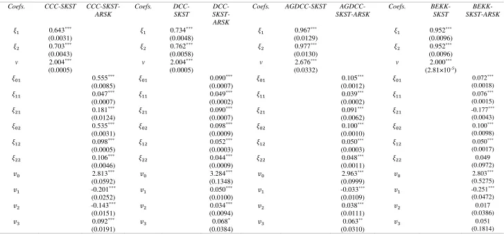
3.2. Static and conditional skewness and kurtosis

Estimates of static parameters for skewness and joint kurtosis in a bivariate SKST

density are reported in Table 210. All the estimates are statistically significant across the

GARCH models, verifying the asymmetry and fat-tailed nature of joint distribution of cash

and futures returns. The logs of skewness parameters 𝜉₁ and 𝜉₂ are both negative, aligning

with the result in Table 1 that the cash and futures returns of Period I are both negatively

9

ADF and PP confirmed that the log index cash and log futures prices are first difference stationary for all the subsamples. Johansen cointegration testing confirmed that the cash and futures prices are cointegrated for the same sub-periods.

10 _{In the interests of brevity, results on the CCC, DCC, AGDCC and BEKK GARCH models are not reported}

17

skewed. The degree of freedom approaches 2, suggesting a large extent of thickness of tails.

It is consistent with the high measure of the fourth moments of cash and futures returns in

Table 1.

[Insert Table 2 about here]

In terms of the autoregressive processes associated with the skewness of marginal

densities and joint kurtosis, the estimates of 𝜉₁₁, 𝜉₂₁, 𝜉₁₂ and 𝜉₂₂ are all significant across the

GARCH models except 𝜉₂₂ by the BEKK model. The skewness of cash (futures) returns is

conditioned on the past shocks and its own lagged values. The result confirms the

autoregressive behaviour of degree of asymmetry. Moreover, the signs of 𝜉₁₁, 𝜉₂₁, 𝜉₁₂ and

𝜉22 are positive, which is also the case with the CCC, DCC, and AGDCC models. Also, 𝜉11

and 𝜉₁₂ are positive for the BEKK model. The positive autocorrelation of third moment of the

S&P 500 cash market is qualitatively consistent with the findings by Jondeau and Rockinger

(2003) with regard to the same market, and with Bali et al. (2008) on the CRSP

value-weighted index. An exception is the negative 𝜉₂₁ attached with the BEKK, suggesting a

negative autocorrelation of cash skewness. The result differs from Jondeau and Rockinger

(2003) and Bali et al. (2008); however, it follows the finding by Harvey and Siddique (1999).

The dynamics of the degree of freedom parameter is revealed by significance of 𝑣₁, 𝑣₂

and 𝑣₃ despite insignificant estimates of 𝑣₂ and 𝑣₃ under the BEKK model. The result

suggests the thickness of tails of the joint distribution of cash and futures markets hinges not

only on the past shocks arising from the two markets but on its lagged own behaviour. Most

of the estimated models agree that the joint kurtosis negatively relates to the past cash shocks

but positively relates to the past futures shocks as well as its lagged own values. A significant

positive autocorrelation of the joint kurtosis consists with the previous findings on the

18

2005; Bali et al., 2008). Overall, Table 2 reveals the existence of conditional autoregressive

processes for skewness and kurtosis parameters in a bivariate density of asset returns11.

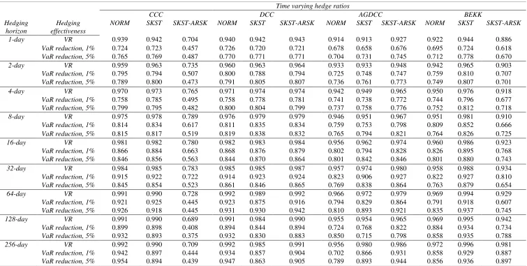
3.3. A comparison of hedging effectiveness

We examine two aspects of the effects of the static and conditional higher order moments

on hedging effectiveness of the conditional optimal hedge ratios. First, we examine how

hedging effectiveness differs across densities under each GARCH model. Second, the

question how the best-performed GARCH model varies across densities is addressed. The

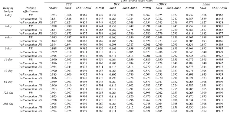
out-of-sample hedging effectiveness of the conditional optimal hedge ratios for a normal

period (i.e. Period II) and a crisis period (i.e. Period IV) is shown horizon-by-horizon in

Table 3 and Table 4, respectively. Note that Period IV is a period of global finance crisis

(GFC).

[Insert Table 3 about here]

In Table 3 under the CCC GARCH model, the SKST density provides the best variance

reduction in 6 out of 9 horizons most of which have short length. Regarding the reduction in

tail risk, the SKST density still performs better than the other two, providing the highest VaR

reduction in 5 out of 9 horizons at both 1% and 5% confidence levels. However, we do not

find evidence that the SKST density with autoregressive skewness and kurtosis parameters

provides benefit for hedging effectiveness under the CCC model. The result from the BEKK

model is similar to that for the CCC. The SKST density performs best in terms of both

variance reduction and VaR reduction in all the horizons. It also can be seen that the SKST

density with autoregressive skewness and kurtosis parameters beats the normal counterpart

for the longest hedging horizon in terms of both variance reduction and VaR reduction.

11 _{The results from Period III are qualitatively similar to those of Period I. To save space, those results are not}

19

Evidence is found under the DCC and AGDCC models in Table 3 that the SKST density

with autoregressive skewness and kurtosis parameters benefits hedging effectiveness for the

conditional optimal hedge ratios. Under the DCC model, the SKST density with

autoregressive skewness and kurtosis parameters performs best in 6 out of 9 horizons in terms

of variance reduction. The performance of the same density in terms of VaR reduction is best

for 3 horizons at 1% and 4 horizons at 5% confidence levels, respectively. An increasing

trend of hedging effectiveness is found for 6 out of 9 horizons across the densities of normal,

SKST, and SKST with autoregressive higher order moments. Most of those horizons are

short ones, ranging from 1-day to 32-days.

The result from the AGDCC model provides stronger evidence. The SKST density with

autoregressive skewness and kurtosis parameters produces the best variance reduction in all

the horizons. It provides the best VaR reduction for 8 horizons at both 1% and 5% confidence

levels. Those horizons range from short to long periods. For all the horizons, hedging

effectiveness increases across the densities of normal, SKST and SKST with autoregressive

asymmetry and thickness of tails.

On average, compared with the normal density, the SKST density increases variance

reduction by around 0.84%. It also increases VaR reduction at 1% and 5% confidence levels

by 2.24% and 2.09%, respectively. The SKST density with autoregressive skewness and

kurtosis parameters further increases variance reduction by 0.68% than the SKST density.

The former increases VaR reduction at 1% and 5% confidence levels by 2.53% and 2.08%

than the latter, respectively.

If we examine how the best-performing model varies across the different densities, the

DCC model performs best for most of hedging horizons under the normal density. When we

20

is true for almost all the horizons. However, when the autoregressive asymmetry and

thickness of tails are taken into account, the DCC model performs best again for all the

horizons. The result implies that the DCC models are seemingly the optimal choice for the

dynamic minimum-variance hedging. It should be cautious that the result is not stable as the

best-performed model varies across different assumptions on the shape behaviour of returns

distribution.

[Insert Table 4 about here]

Regarding the effects of higher order moments on the conditional optimal hedge ratios,

the results for the GFC period are shown in Table 4. A monotonic growth of both variance

and VaR reductions is evident across the different density functions using the CCC, DCC,

and AGDCC models, and is the case for most of the hedging horizons. Under each GARCH

model, the normal density is dominated by the other two density functions for most hedging

horizons. Under the BEKK model, an increase of hedging effectiveness is valid only for 2

horizons. However, the SKST density still performs best, which is evidenced in 4 out of 6

hedging horizons. In addition, the SKST density with autoregressive skewness and kurtosis

parameters outperforms normality for all the horizons.

On average, it is found that the SKST density function can improve variance reduction

by around 3.11% than the Normal counterpart. The former also increases VaR reduction by

6.99% and 6.10% at the 1% and 5% confidence levels over the Normal, respectively.

Compared with the static higher order moments, the autoregressive cases further increase

variance reduction by 0.80%, VaR reduction at 1% level by 2.69% and VaR reduction at 5%

level by 2.46%, respectively. This result indicates the benefit of incorporating the

autoregressive behaviour of higher order moments on hedging performance of dynamic

21

period. Hence the conditional higher moments are helpful for improving the quality of risk

management in light of volatility minimisation and tail risk reduction, especially during a

crisis period.

Table 4 reports a different result for the variation of the best-performing model across

densities than that reported in Table 3. The best model under normality is the CCC in terms

of both variance and VaR reductions for all the horizons. BEKK performs best when the

SKST density is employed. The best performance of the BEKK model is evident for most of

horizons. However, when allowing the higher order moments to be autoregressive, we find

DCC performs best for relatively short horizons (1-day, 2-day, 4-day, and 8-day) whereas

BEKK performs best for relatively long ones (16-day and 32-day). Thus, the variation of the

best-performed model across densities during GFC is more substantial than during a normal

period. Our result suggests that the BEKK and DCC models might be rational choices on the

dynamic minimum-variance hedging strategies during a crisis period. However, it should be

kept in mind that the pattern of returns distribution has an impact on those choices. Such

impact is valid irrespective of when the hedging activities take place.

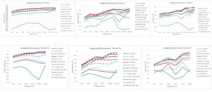
[Insert Figure 1 about here]

Figure 1 indicates that when the hedging horizon increases, most hedge ratio series

exhibit a growing trend of hedging effectiveness which is roughly monotonic. The growth of

hedging effectiveness along with an increase of hedging horizon in length is witnessed for

both normal and crisis periods, which is consistent with previous studies (e.g. Ederington,

1979; Geppert, 1995; Chen et al., 2004; Lien and Shrestha, 2007; Lai and Sheu, 2010).

Moreover, we can consistently observe from the figure that the conditional hedging ratios

derived from the densities with the static and conditional higher order moments possess lines

22

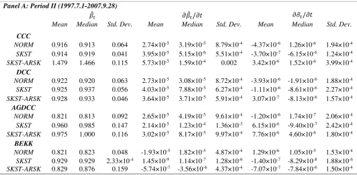
3.4. Relations between hedge ratio and hedging effectiveness

In this subsection we examine how the relations between several statistical properties of

the conditional hedge ratios and hedging effectiveness differ across different conditional

densities. The statistical properties of the conditional hedge ratios under question include the

mean, standard deviation, smoothness of ratio series and smoothness of standard deviation.

Note the latter three properties contribute towards explaining the stability of series of

conditional hedge ratios. The smoothness of ratio series is measured by the standard deviation

of the partial first derivatives of hedge ratios over time. Likewise, we use the standard

deviation of the partial first derivatives of hedge ratios’ standard deviation over time as a

proxy for the smoothness of ratio standard deviation12. Note that the standard deviation of the

partial first derivatives measures the average dispersion of changes of the time series over

time. If the standard deviation equals zero, the change is fixed and the series is a linear

function of time. Hence one intuitively expects that the lower the standard deviation, the

higher the series’ smoothness. The properties of the conditional hedge ratios for both Period

II and Period IV are summarised in Table 5.

[Insert Table 5 about here]

We examine whether the conditional hedge ratios derived by the best

(worst)-performed hedging model under each density possess the shortest (longest) distance of the

mean to unity, the smallest (largest) standard deviation, the highest (lowest) ratio smoothness

and the highest (lowest) smoothness of ratio standard deviation. Evidence is revealed for

Period II and Period IV, respectively.

12 _{The partial first derivative over time is an estimate of coefficient of the time trend in a regression model}

23

We find from Period II that the best model under normality, i.e. the DCC model, yields

ratios the mean of which is closest to unity. However, they have the second smallest standard

deviation and second highest smoothness of ratios and standard deviation. The situation gets

better when moving to the SKST density where the ratios generated by the best model under

that density (BEKK model) possess the smallest standard deviation and highest smoothness

of ratios and standard deviation. However, the SKST density with autoregressive higher order

moments only confirms that the best model produces the least volatile ratio series. The

argument that the ratios that are closest to unity have the best performance is not supported

by the densities with static and conditional higher order moments.

The results concerning the properties of ratios derived by the worst models are clearer.

Staying with Period II, the worst model under normality (CCC model) produces the ratios

with the longest distance of mean to unity, smallest standard deviation and lowest smoothness

of ratio and standard deviation series. The finding is confirmed by the densities with static

and conditional higher order moments. Thus, results from Period II reveal that the SKST

density reinforces the fact of a positive relation between stability of hedge ratios and hedging

effectiveness than the normal counterpart.

The results from Period IV reinforce these findings. Results based on all the density

functions concur that the ratio series with its mean closest to unity has the best effectiveness.

Only the SKST density function finds that the worst performance relates to the longest

distance of the mean from unity. The Normal and SKST density function with autoregressive

higher order moments supports the case that the least (most) volatile ratios with highest

(lowest) smoothness are best (worst) performing. The SKST density function with

autoregressive higher order moments further finds that the highest (lowest) smoothness of

standard deviation of ratios series contributes to the best (worst) hedging effectiveness. In

24

higher stability of hedge ratios leads to better hedging effectiveness. The result enhances the

findings by the previous studies on the relationship between conditional hedge ratio and

hedging effectiveness (e.g. Park and Jei, 2010; Lien, 2010; Hou and Li, 2013; Kim and Park,

2016).

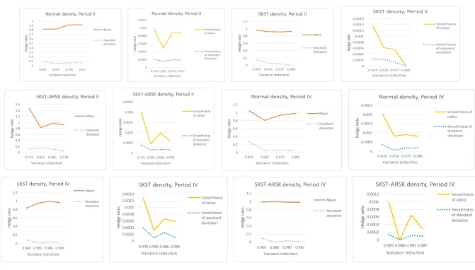
[Insert Figure 2 about here]

The relations between different statistical properties of hedge ratios and average hedging

effectiveness over all the hedging horizons are plotted in Figure 213. The figure shows how

those properties change with average hedging effectiveness across the GARCH models under

each density function. As can be seen from the figure, the average hedging effectiveness

increases as the hedge ratio means approach unity. This is for all densities in both Period II

and Period IV. The volatility of ratio series appears negatively related to hedging

effectiveness where the lower the volatility, the better the effectiveness. In addition, there are

rough downward trends for the standard deviations of the partial first derivatives of the ratios

series and their standard deviations over time, and the average hedging effectiveness. The

downward trends indicate a positive relationship between the smoothness of ratio series and

volatility and hedging effectiveness. We find those trends are more highlighted under the

SKST densities with static and autoregressive higher order moments despite some of them

not being monotonic. Indeed, so is the negative relation between volatility and hedging

effectiveness. The result based on the analysis of the average hedging effectiveness is

consistent with that based upon the best (worst) performed hedging models.

3.5. Hedge ratio and higher order moments

The effects of higher order moments on the statistical properties of conditional hedge

ratios are further explored in this subsection. Those effects are qualitatively described by

13 _{The properties are plotted against variance reduction in the figure. The plots with VaR reduction on the X axis}

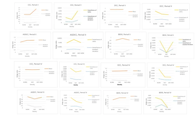
25

Figure 3. This figure depicts how the mean, standard deviation, smoothness of ratio series

and their standard deviations vary across different densities under each GARCH model. As

mentioned earlier, smoothness is measured by the standard deviation of the partial first

derivatives of time series over time.

[Insert Figure 3 about here]

As can be seen from the figure, there is an upward trend in the mean for 6 out of 8 plots.

The mean normally converges to unity. It suggests that taking into account the static and

conditional higher order moments may monotonically increase the mean of hedge ratios when

it is below 1. The standard deviation of ratios moves continuously downward when the

densities with the static and conditional higher order moments are chosen. It is confirmed in 5

out of 8 plots. Moreover, a monotonic downward trend of standard deviations of the partial

first derivatives of ratios and their standard deviations over time is respectively detected by 5

and 6 out of 8 plots when moving across the X axis from left to right. It suggests smoothness

of series may be consistently enhanced by higher order moments and their autoregressive

feature.

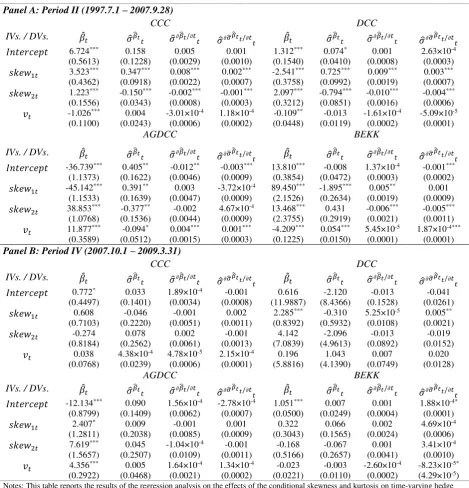
To explore the quantified effects, we estimate the following equations:

𝛽̂𝑡 = 𝑖𝑛𝑡𝑒𝑟𝑐𝑒𝑝𝑡 + 𝛼1𝑠𝑘𝑒𝑤1𝑡 + 𝛼2𝑠𝑘𝑒𝑤2𝑡 + 𝛼3𝑣𝑡+ 𝑒𝑡,

𝜎̂𝛽̂𝑡_𝑡= 𝑖𝑛𝑡𝑒𝑟𝑐𝑒𝑝𝑡 + 𝛽₁𝑠𝑘𝑒𝑤_1𝑡 + 𝛽₂𝑠𝑘𝑒𝑤_2𝑡 + 𝛽₃𝑣_𝑡+ 𝑒_𝑡,

𝜎̂𝜕𝛽̂𝑡/𝜕𝑡_𝑡= 𝑖𝑛𝑡𝑒𝑟𝑐𝑒𝑝𝑡 + 𝛾₁𝑠𝑘𝑒𝑤_1𝑡 + 𝛾₂𝑠𝑘𝑒𝑤_2𝑡 + 𝛾₃𝑣_𝑡+ 𝑒_𝑡,

𝜎̂𝜕𝜎̂𝛽̂𝑡𝑡/𝜕𝑡_𝑡 = 𝑖𝑛𝑡𝑒𝑟𝑐𝑒𝑝𝑡 + 𝛿₁𝑠𝑘𝑒𝑤_1𝑡 + 𝛿₂𝑠𝑘𝑒𝑤_2𝑡 + 𝛿₃𝑣_𝑡+ 𝑒_𝑡. (16)

where 𝛽̂_𝑡 denotes the estimated conditional optimal hedge ratios; 𝜎̂𝛽̂𝑡_{𝑡 represents the series of}

26

deviations of 𝜕𝛽̂_𝑡/𝜕𝑡 and 𝜕𝜎̂𝛽̂𝑡_𝑡/𝜕𝑡_{, respectively.} 𝜕𝛽̂_𝑡/𝜕𝑡 _and 𝜕𝜎̂𝛽̂𝑡_𝑡/𝜕𝑡 _{are the partial first}

derivatives of 𝛽̂_𝑡 and 𝜎̂𝛽̂𝑡_{𝑡 over time, respectively. Time variation of} 𝜎̂𝜕𝛽̂𝑡/𝜕𝑡_{𝑡 and} 𝜎̂𝜕𝜎̂𝛽̂𝑡𝑡/𝜕𝑡_𝑡

is obtained by the rolling window mechanism with window size 100 observations and step

size 1 observation. 𝑠𝑘𝑒𝑤_1𝑡 and 𝑠𝑘𝑒𝑤_2𝑡 are the conditional skewness measures for marginal

densities of cash and futures returns in a bivariate SKST distribution, respectively.

𝑠𝑘𝑒𝑤𝑖𝑡 = 𝜉2_𝑖𝑡(𝑖 = 1,2 ) and 𝜉 _𝑖𝑡 is an autoregressive skewness parameter that is an

exponential function of 𝜉̃_𝑖,𝑡 defined as in Eq. (8). The sign of 𝑠𝑘𝑒𝑤_𝑖𝑡 is determined by

𝑙𝑛 (𝜉 _𝑖𝑡) where 𝑠𝑘𝑒𝑤_𝑖𝑡 is positive (negative) when 𝑙𝑛(𝜉 _𝑖𝑡) > 0 (< 0) . 𝑣_𝑡 is the

conditional degree of freedom of the bivariate SKST density. 𝑣_𝑡 is an exponential function of

𝑣̃𝑡 defined as in Eq. (9). Data of Period II and IV are employed for estimating Eq. (16),

respectively. Estimation results are separately obtained for the CCC, DCC, AGDCC and

BEKK GARCH models for each period, which are shown in Table 6.

[Insert Table 6 about here]

As can be seen from the table, the marginal skewness of futures returns promotes the

size of hedge ratio, which is indicated by all the positive significant estimates. The same

effect is also rendered by the marginal skewness of cash returns, which is suggested by 4 out

of 6 positive significant estimates. The effect from the joint kurtosis is negative given that 3

out of 5 estimates are significant negative. However, the joint effect of skewness and

kurtosis on the size of hedge ratio is positive, suggesting that higher order moments of a

bivariate distribution escalate the conditional hedge ratios.

Significant effects of higher order moments on the volatility of conditional hedge ratios

are found only for Period II. The marginal skewness of futures market decreases the volatility

whereas that of cash market does in a reverse way. The argument is supported by most of

27

estimate is positive while the other is negative. However, an agreement can be achieved that

the joint effect of skewness and kurtosis is negative if the individual effects are summed. The

supporting evidence is found in the estimation under the DCC, AGDCC and BEKK models.

The result implies that taking into account the higher order moments helps to gauge less

volatile hedge ratio series.

Lastly, the marginal skewness of cash returns downgrades the smoothness of hedge ratio

and its volatility whereas that of futures returns elevates it. This is supported by the

estimation results under the CCC, DCC and BEKK models. Meanwhile, the joint kurtosis

decreases the smoothness of relevant series, suggested by the results under the AGDCC and

BEKK models. However, the aggregate effect suggests that the smoothness of both ratio and

volatility series is enhanced when both skewness and kurtosis are taken into account.

The finding is useful in explaining why the SKST density with the static and

autoregressive skewness and kurtosis parameters improves hedging effectiveness of

conditional optimal hedge ratios than the normality. The reasoning is that the higher order

moments produce hedge ratios with larger size and higher stability and consequently those

ratios possess higher hedging effectiveness. Likewise, the autoregressive higher order

moments generate higher effectiveness than the static ones since the hedge ratios estimated

by the former possess larger size and higher stability.

3.6. Robustness check on hedging effectiveness

We examine whether the effects of the static and autoregressive higher order moments on

hedging effectiveness during a post-GFC period are similar to those of pre- and during-GFC

periods14. In doing this, we collect a sample of daily closing (settlement) prices of the S&P

14 _{A robustness check was also conducted on the effects of the higher order moments on the relations between}

28

500 cash (futures) from April 1, 2009 to March 30, 2017. We end up with 2087 observations

for the sample. Following the analysis on the pre-GFC period, the out-of-sample hedging

effectiveness of the CCC, DCC, AGDCC, and BEKK GARCH hedge ratios is assessed for 9

hedging horizons15. The results are shown in Table 7.

[Insert Table 7 about here]

On one hand, the table shows a monotonic increase in variance reduction when moving

across the densities of normality, SKST, and SKST with autoregressive skewness and

kurtosis parameters. Such increase is evidenced by all the hedging horizons of the CCC

hedge ratios and 8 out of 9 horizons of the AGDCC and BEKK ratios. Likewise, a monotonic

growth of VaR reduction exists, which is agreed by 9 horizons of the CCC, 8 horizons of the

BEKK, and 6 horizons of the AGDCC. Although the DCC hedge ratios do not witness the

superiority of the autoregressive higher order moments in hedging effectiveness, they

strongly support that the static higher order moments yield higher effectiveness than the

normality for most of hedging horizons. On average, compared to the normality, the static

higher order moments increase variance reduction by around 2.52%, VaR reduction at the 1%

level by around 9.45%, and VaR reduction at the 5% level by around 3.97%. The

autoregressive counterparts further increase variance reduction by around 0.57%, VaR

reduction at the 1% level by around 2.50%, and VaR reduction at the 5% level by around

3.45%. The post-GFC results are similar to those of the other periods reported in this paper.

On the other hand, it is found the evidence that the static and autoregressive higher order

moments affect the choice on the best-performed hedging model. The CCC GARCH model

keeps performing best across all the hedging horizons under normality. This situation varies

when turning to the SKST density where the BEKK model is the best for all the horizons.

This choice rarely changes when the skewness and kurtosis are time varying. Hence the

29

GFC evidence consists with that of the pre- and during-GFC periods given that taking into

account the static and autoregressive higher order moments impacts the decision on the

dynamic hedging model. The result also points to a change of the best-performed model from

pre- to post-GFC periods. That is, the DCC model might be the best before the crisis while

the BEKK takes the lead after that.

4. Concluding remarks

Although dynamic minimum-variance futures hedging has been widely investigated in

the literature, the effects of non-standard tail behaviour of asset returns on conditional hedge

ratio remain unclear. This paper explores three aspects important aspects of this issue: (i)

whether the bivariate skew-Student density functions with the static and autoregressive third

and fourth moments improves hedging effectiveness over the Normal distribution; (ii)

whether the density functions matters in terms of the relationship between hedge ratio and

hedging effectiveness; and (iii) whether the density functions impact on the time varying

features of ratio series.

Compared to the Normal density, there is evidence that the density functions with the

static higher order moments increases both variance and VaR reduction. Compared to the

static counterpart, the autoregressive higher moments can further increase the same metrics.

A monotonic increase in hedging effectiveness from the normal to the non-normal densities is

evidenced by at short and long hedging horizons. These findings are obtained for both

tranquil and GFC periods. Those improvements imply that taking into account the static and

conditional higher order moments of asset returns benefits risk management. Moreover, this

paper reveals that the best-performing hedging model varies across different densities. An

30

decision on the choice of a best dynamic hedging strategy. The results of the effects of higher

order moments on hedging effectiveness are robust in a post-GFC period.

The relations between conditional hedge ratio and hedging effectiveness are revealed that

higher magnitude and stability of ratio series lead to better effectiveness. The stability is

reflected by volatility and smoothness of ratio and volatility series. This finding is enhanced

by the static and autoregressive higher order moments. Furthermore, significant evidence

suggests that the static and conditional higher order moments contribute to the size and

stability of conditional hedge ratios. This can thus serve as a reason behind on the

31

Appendix 1 Proofs of a quantitative relationship between the higher moments of a minimum variance hedge portfolio and the optimal hedge ratio

The proof that the third moment of a minimum variance hedge portfolio is a function of the optimal hedge ratio is given by Fu (2014, pp 214).

The proof for the fourth moment stems from Fu (2014). Suppose a minimum variance hedge

portfolio is constructed by

𝑅_ℎ = 𝑅_𝑠 − ℎ 𝑅_𝑓. (A1.1)

where 𝑅_ℎ, 𝑅_𝑠 and 𝑅_𝑓 are returns of hedge portfolio, unhedged position and futures,

respectively. ℎ is the minimum variance hedge ratio. From Eq.(A1.1), the fourth moment of

𝑅ℎis derived by

𝑢4(𝑅ℎ) = 𝐸[𝑅ℎ− 𝐸(𝑅ℎ)]4

= 𝐸{𝑅_𝑠− 𝐸(𝑅_𝑠) − ℎ [𝑅_𝑓− 𝐸(𝑅_𝑓)]}4

= 𝐸[𝑅_𝑠− 𝐸(𝑅_𝑠)]4− 2ℎ𝐸{[𝑅_𝑠− 𝐸(𝑅_𝑠)]3[𝑅_𝑓− 𝐸(𝑅_𝑓)]} + 2ℎ2𝐸 {[𝑅_𝑠−

𝐸(𝑅𝑠)]2[𝑅𝑓− 𝐸(𝑅𝑓)]2} − 2ℎ3𝐸 {[𝑅𝑠− 𝐸(𝑅𝑠)] [𝑅𝑓− 𝐸(𝑅𝑓)]3} +

ℎ4_𝐸[𝑅

𝑓− 𝐸(𝑅𝑓)]4.

where the fourth and co-fourth moments of the cash and futures returns are defined by

𝑢4(𝑅𝑠) = 𝐸[𝑅𝑠− 𝐸(𝑅𝑠)]4,

𝑢4(𝑅𝑓) = 𝐸[𝑅𝑓− 𝐸(𝑅𝑓)]4,

𝑢3,1 = 𝐸{[𝑅𝑠− 𝐸(𝑅𝑠)]3[𝑅𝑓− 𝐸(𝑅𝑓)]},

𝑢2,2 = 𝐸 {[𝑅𝑠− 𝐸(𝑅𝑠)]2[𝑅𝑓− 𝐸(𝑅𝑓)]2},

𝑢1,3 = 𝐸 {[𝑅𝑠 − 𝐸(𝑅𝑠)] [𝑅𝑓− 𝐸(𝑅𝑓)]3}.

Then we have

𝑢₄(𝑅_ℎ) = 𝑢₄(𝑅_𝑠) − 2ℎ𝑢_3,1+ 2ℎ2𝑢_2,2− 2ℎ3𝑢_1,3+ ℎ4𝑢₄(𝑅_𝑓). (A1.2)

Eq.(A1.2) clearly shows that 𝑢₄(𝑅_ℎ) is a function of ℎ, the fourth moments and the co-fourth