Munich Personal RePEc Archive
Follow the Value Added: Tracking
Bilateral Relations in Global Value
Chains
Borin, Alessandro and Mancini, Michele
Bank of Italy, Bank of Italy
14 November 2017
Follow the Value Added:
Tracking Bilateral Relations in Global Value
Chains
Alessandro Borin and Michele Mancini*
(first version June 2015, this version November 2017)
Abstract
Following the spread of global value chains new statistical tools, the Inter-Country Input-Output tables, and new analytical frameworks have been recently developed to provide an adequate representation of supply and demand linkages among the economies. Koopman, Wang and Wei propose an innovative accounting methodology to decompose a country’s total gross exports by source and final des-tination of their embedded value added. However this decomposition presents some limitations and relevant inexactnesses in some of its components. We develop their approach further by deriving a fully consistent counterpart for bilateral trade flows, also at the sectoral level, addressing the main shortcomings of previous works. We also provide correct breakdown of the foreign content in total (world) trade flows and a brand new classification of these components that take the perspective of the exporting country. Finally, drawing on our methodology we derive for the first time a precise measure of international trade generated within global production networks. Two examples of empirical applications with relevant policy implications are also provided.
Keywords: global value chains; input-output tables; trade in value added; trade elasticity. JEL classification: E16, F1, F14, F15.
*Bank of Italy. alessandro.borin@bancaditalia.it, michele.mancini@bancaditalia.it.
1
Introduction
The international fragmentation of production processes has challenged the capability of the stan-dard trade statistics to truly represent supply and demand linkages among economies. In general bilateral exports differ from the portion of a country’s GDP related with the production of goods and services shipped to a certain outlet market. On one hand exports also embed imported inter-mediate inputs, on the other hand the directly importing country often differs from the ultimate destination where the good is absorbed by final demand. Whenever production is organized in se-quential processing stages in different countries, trade statistics repeatedly double-count the same value added. The diffusion of global value chains (GVC) has therefore deepened the divergence between gross flows, as recorded by traditional trade statistics, and the data on production and final demand as accounted for in statistics based on value added (above all GDP). Moreover, own to the spread of GVC, new relevant questions regarding the role of countries and sectors in the international markets have emerged. In particular, it has become crucial to assess the level of participation of countries and sectors into the international sharing of production.
New data, as the Inter-Country Input-Output tables, and new analytic methodologies have been developed in order to address these issues. Among the latter Koopman, Wang and Wei (2014) (hereafter KWW) propose a comprehensive decomposition of total gross exports by the source and destination of their embedded value added, that encompasses most of the methodologies previously proposed in the literature (e.g. Hummels et al. 2001; Daudin et al., 2009; and Johnson and Noguera, 2012). KWW point out that different schemes of international fragmentation of production yield different proportions of value added content in gross exports. In particular, they show that not all the double-counted flows in gross trade statistics are alike.
More specifically, KWW break gross exports down into different components of domestic and foreign value added plus two items of “pure” double counting. As to the latter, they show that gross exports do not in general consist only of value added that can be traced back to GDP generated either at home or abroad. Instead, some trade flows are purely double-counted, as when intermediate inputs cross a country’s borders several times according to the different stages of production.1
It is worth noting that these double-counted items are increasingly important in international trade flows (see Wang et al., 2013 and Cappariello and Felettigh, 2015), making the KWW approach particularly valuable.
Albeit providing useful insights, the original KWW decomposition still presents some relevant shortcomings and limitations. They correctly measure the total domestic value added in exports, but the breakdown by destination market is imprecise. Furthermore their measures of the value added generated abroad and of the foreign double counted items in total exports are incorrect, since they overstate the latter component.2
More in general the KWW decomposition finds limited scope for empirical applications since it neglects the bilateral and sectoral dimensions of trade flows. It means, for instance, that it can not be applied to analyze all the direct and indirect linkages between countries and sectors within the production networks. Another relevant limitation is that we can not get a precise measure of the share of total trade that is related to
1
A more detailed account of this mechanism is provided in section 2.2, where we discuss the differences between the sink and the source approaches of the bilateral decomposition.
2
GVC participation from the standalone application of the KWW decomposition.
Besides these issues there are several other reasons why we might be interested in tracing value added flows between countries. In fact firms trade with bilateral partners, even when par-ticipating in more complex multi-country production networks. In studying GVC, it is relevant to analyze the overall structure of production networks and to identify all the international and inter-sectoral links. Methodologies like KWW’s can track the value added linkages between the country of origin and the final destination. But we may also be interested in the position of a country (or a sector) within the production process and in identifying its direct upstream and downstream trade partners. This might be relevant in order to map geographically the production networks and to analyze the international propagation of macroeconomic shocks, as exchange rates’ varia-tions. Deepening the knowledge of these mechanisms also provides useful insights to interpret the short-term dynamics of trade flows.3
Moreover, countries’ participation in GVCs affects bilateral trade balances (Nagengast and Stehrer, 2016); this and other features of bilateral shipments, as their merchandise composition, unambiguously influence trade policies (e.g. international trade and investment agreements). More in general, the potential policy implications of all the aspects mentioned above are clearly significant.
Our aim is to extend KWW’s methodology in order to obtain a consistent decomposition of bilateral (and sectoral) trade flows that offers additional information on a good many matters that cannot be investigated using simple gross trade data or aggregate trade in value added. For instance, by considering the bilateral dimension of trade-production relations it is possible to measure the amount of trade generated within global production networks.
We also intend to overcome shortcomings and limitations that affect the KWW decomposi-tion and other previous attempts to get a bilateral counterpart of the KWW scheme. In particular we provide proper definitions for some components that are incorrectly specified by KWW: i) the domestic value added that is directly (and indirectly) absorbed by the final demand of the import-ing country; ii) the foreign value added (FVA) in exports; iii) the double counted items produced abroad. At the world level our corrected variant of the KWW’s FVA component resembles the measure proposed by Johnson (2017), which is derived in a completely different framework. Indeed the two measures do not coincide when computed for a single exporting country.4
Beside improving the measures of FVA and foreign double counted (FDC) within the KWW framework, we also propose a completely alternative approach to split these two compo-nents. According to the KWW logic, which in this aspect is shared also by Johnson (2017), FVA and FDC are defined referring to world trade flows.5
However, from the perspective a particular
3
Although ICIO data are only available with a lag, we can still use these tools to interpret and project short-term developments in international trade, insofar as the value added structure of bilateral exports is quite persistent over time. For example, if we know that in motor vehicles manufacturing a considerable share of the intermediate components exported from Italy to Ger-many are used to produce cars for the North American market, we presume that a slackening of US demand is likely to result in a reduction in shipments of parts from Italy to Germany.
4
We also present an extended version of the FVA indicator proposed by Johnson (2017), with a breakdown by country of ultimate destination.
5
exporting country this might not be economically meaningful and it produces an arbitrary allo-cation of trade flows, depending on the number of upward (or downward) stages of production that stand between the exporter and the country in which the value added was generated (or the market of final destination). In order to address this issue we propose two brand new measures of FVA and of FDC consistent with those adopted for the domestic content of exports. As better explained later on, these measures can be derived in different ways for bilateral trade flows, then generating distinct results at this level of disaggregation. Nevertheless, they all sum up to the same indicators of FVA and of FDC when computed at the country level.
We also overcome the main problems that make imprecise and at least partially incorrect the value added decompositions of bilateral exports previously proposed in the literature. In this regard our work is related to that of Nagengast and Stehrer (2016) and Wang et al. (2013). Nagengast and Stehrer (2016) point out that there are different ways to account value added in bilateral trade. Indeed they propose two alternative methodologies: a first one takes the perspective of the country where the value added originates (the source-based approach), a second one takes the perspective of the country that ultimately absorbs it in final demand (the sink-based approach). However, neither methodology in Nagengast and Stehrer (2016) are correctly specified, so that they do not include the entire domestic value added embedded in each bilateral trade flow. We propose two alternative breakdowns of bilateral exports that overcome this shortcoming, while maintaining two separate frameworks for the source-based decomposition and for the sink-based one. Both our decompositions correctly take into account the domestic value added, the foreign value added and the double-counted components of bilateral exports. In both cases there is a precise correspondence with the items in the KWW decomposition when we consider the total exports of a country (apart from the components that are erroneously defined in KWW). Having specific and internal consistent methodologies both for the sink-based and the source-based approach allows to choose the most appropriate framework to the purpose of the analysis.
Wang et al. (2013) follow KWW closely and propose a single breakdown of bilateral exports that can be exactly mapped into the original KWW decomposition summing all the export flows across the destinations. This also means that the drawbacks of the KWW methodology mentioned above apply also this bilateral variant (e.g. the incorrect identification of of the foreign value added component). Moreover, Wang et al. (2013) mix sink and source approaches to single out the different components, so that their methodology suffers from internal inconsistency. Finally and more importantly, they can not identify the trade flows that are generated within global supply networks, which has emerged as a key question in the literature. According to the definition first proposed by Hummels et al. (2001) and commonly acknowledged in this field, GVC schemes should entail at least two separate production stages in different countries, before the good is ultimately shipped toward the final market. In other words there should be at least a re-shipment of intermediate or final goods toward a third country (or back to the country of origin). Conversely, ‘traditional’ production and trade patterns result in goods and services produced in a certain country and consumed by the direct importer. Wang et al. (2013) methodology, which in part follows a sink-based approach, does not allow to distinguish between these two cases, while our source-based decomposition is suited to tackle this issue. Indeed in section 3.2 we propose for the first time a measure of GVC-related trade that is consistent with Hummels et al. (2001)
definition, providing empirical evidence about its evolution at the global level.
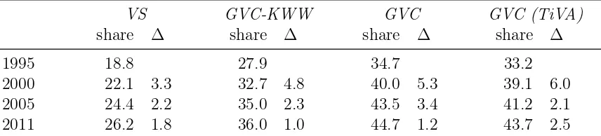
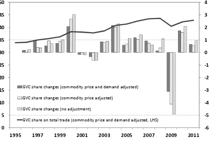
While we show a couple of possible implementations of our decompositions by using ICIO tables (the World Input Output Database, WIOD, and the OECD-WTO Trade in Value Added, TiVA) the detailed breakdown of bilateral/sectoral gross exports presented here might find a much broader scope for empirical investigations on global production networks. In particular, it provides the basic information needed to assess country/sector position and participation in GVCs and to develop measures about the overall lengths of international supply chains (Antràs and Chor, 2013; Wang et al., 2016; Borin and Mancini, 2016). In this way it will be possible to investigate at the macro (country-sector) level some features of production networks that have emerged from case studies (Dedrick et al., 2010; Ivarsson and Alvstam, 2011) and firm level analyses (Sturgeon et al., 2008, Brancati et al., 2017).
The rest of the paper is organized as follows. The second section recalls KWW’s account-ing, presents two novel decompositions of bilateral exports that overcome the main drawback in KWW’s methodology, proposes an alternative approach to account for the foreign value added in exports, illustrates how to include three different sectoral dimensions in the decompositions and discusses how these new tools can contribute to analyze international production networks. The third section shows two empirical applications: the first one adopts the sink-based approach to explore the forward linkages of the world’s largest exporters; the second one takes the source-based perspective to derive a measure of GVC-related trade and to assess how its evolution since the mid-1990s has affected the relationship between world trade and income. Section four concludes.
2
The decomposition of bilateral gross exports
2.1
KWW’s breakdown of total exports
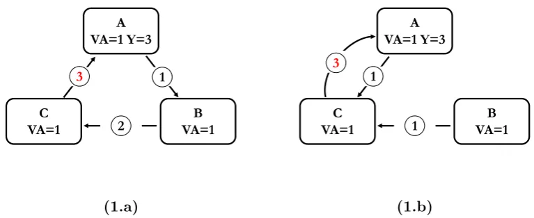
The methodology proposed by KWW constitutes a innovative and comprehensive accounting framework for gross foreign trade. The way in which this tool can improve our evaluation of countries’ trade relationships is offered by the two stylized production-consumption-trade schemes shown in Figure 1. In panel 1.a) production is organized in stages, each in a different country. First country A produces 1 USD worth of intermediate components using only its own resources and ships them to B, which adds 1 USD of value to produce more refined intermediate products, which are sent to C. Here they undergo a final processing stage, worth another 1 USD, before being sold as final goods back to A for 3 USD. In panel 1.b, instead of having sequential stages of production in A and B, initially each country produces intermediate components worth 1 USD using only its own productive factors and ships them to C; here the different inputs are assembled, adding another 1 USD of value to produce final goods that are absorbed by final demand in A, as before.
Gross trade statistics indicate that in case 1.a country A’s exports are generated by de-mand from country B, and in case 1.b. by dede-mand from C. Since KWW trace both the origin and the final destination of value added, however, their decomposition shows that in both cases the exports are actually activated by country A’s own domestic demand.
exports introduced by Koopman, Wang and Wei (2014). Their methodology is based on a global input-output model withGcountries andN sectors (for details see Appendix A which also gives an exhaustive definition of our notation, which is essentially identical to KWW). Here let us only recall thatYsr indicates the demand vector of final goods produced ins and consumed inr, B
is the global Leontief inverse matrix for the entire inter-country model,Ais the global matrix of
input coefficients,Vsincorporates the value added shares embedded in each unit of gross output
produced by countrys,Es∗ is the vector of total exports of countrysfor theN sectors, anduN
is the1×N unit row vector.
The essential decomposition of total exports of countrys(uNEs∗) in KWW is summarized
by the following accounting relationship:
uNEs∗ =
Vs
G
X
r6=s
BssYsr+Vs
G
X
r6=s
BsrYrr+Vs
G
X
r6=s G
X
t6=s,r
BsrYrt
+ Vs
G
X
r6=s
BsrYrs+Vs
G
X
r6=s
BsrArs(I−Ass)−1Yss
+ Vs
G
X
r6=s
BsrArs(I−Ass)−1Es∗
+ G X
t6=s G
X
r6=s
VtBtsYsr+
G
X
t6=s G
X
r6=s
VtBtsAsr(I−Arr)−1Yrr
+ G X
t6=s G
X
r6=s
VtBtsAsr(I−Arr)−1Er∗ (1)
KWW defines the nine items in equation (1) as follows:
1. VsPG
r6=sBssYsr: domestic value added in direct final goods exports;
2. VsPG
r6=sBsrYrr: domestic value added in intermediate exports absorbed by direct
im-porters;
3. VsPG
r6=s
PG
t6=s,rBsrYrt: domestic value added in intermediate goods re-exported to third
countries;
4. VsPG
r6=sBsrYrs: domestic value added in intermediate exports reimported as final goods;
5. VsPG
r6=sBsrArs(I−Ass)−1Yss: domestic value added in intermediate inputs reimported
as intermediate goods and finally absorbed at home;
6. VsPG
r6=sBsrArs(I−Ass)−
1E
s∗: double-counted intermediate exports originally produced
at home;
7. PGt6=sPGr6=sVtBtsYsr: foreign value added in exports of final goods;
8. PGt6=sPGr6=sVtBtsAsr(I−Arr)−1Yrr: foreign value added in exports of intermediate goods;
9. PGt6=sPGr6=sVtBtsAsr(I−Arr)−1E
r∗: double-counted intermediate exports originally
Although KWW’s methodology allows to improve the knowledge of value added content of total exports, it provides no insight into the structure of single bilateral flows. As already mentioned, from a policy perspective this could be relevant for several reasons. Consider, for example, the assessment of bilateral trade balances. In Figure 1.a A runs a 1 USD surplus with B and a 3 USD deficit with C, all evaluated in terms of gross trade flows; in case 1.b, A shows a net bilateral balance of -2 USD towards C and zero with respect to B. However, in value added terms, A has a net trade deficit position of 1 USD with B and C in both panels. Thus while A’s overall deficit is exactly the same in value added as in gross terms (2 USD), its bilateral positions differ considerably between the two accounting methods. Using basic accounting relationships and inter-country I-O tables, we can compute the bilateral positions in value added terms.6
Yet this is not enough to disentangle the international production linkages and the ultimate demand forces that generate a particular surplus/deficit between two countries in gross terms; nor does the original KWW breakdown shed light on these matters when multiple trade partners and sources of final demand are involved.
Moreover some of KWW’s definitions are questionable and, to some extent, incorrect, but this will become clear by going though the analysis of bilateral trade flows, so we prefer to discuss these issues in the following sections.
C VA=1
B VA=1 A
VA=1 Y=3
3 1
2
(1.a)
C
VA=1
B
VA=1 A
VA=1 Y=3
1
1
3
[image:8.595.105.489.370.527.2](1.b)
Figure 1:
Value added versus gross export accounting of bilateral trade balances
2.2
The decomposition of bilateral trade
By focusing on bilateral trade flows we can follow the pattern of value added in exports along the different phases of the value chain. However the input-output framework potentially allows for infinite rounds of production. Hence we face a trade-off between adding details about the international production linkages and providing an analytically tractable and conceptually intel-ligible framework. Our compromise is to track the direct importing country, then - if the value added is not absorbed there - we consider the additional destinations of re-export from the direct importers.
6
In summary, our strategy is to decompose gross bilateral trade flows identifying the fol-lowing actors: i) the country of origin of value added;ii) the direct importers;iii) the (eventual) second destination of re-export; iv) the country of completion of final products;v) the ultimate destination market.
C VA=0 Y=3
B VA=1 A
VA=1+1=2
3 1
[image:9.595.212.382.172.285.2]2
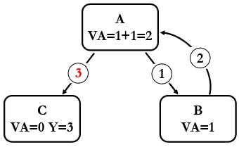
Figure 2:
Value added and double counting in bilateral trade flows
Another conceptual issue that arises in considering the single bilateral flows regards the purely double counted items. As pointed out by Nagengast and Stehrer (2016), when a certain portion of value added crosses the same border more than once it has to be assigned to a particular gross bilateral trade flow, while it should be recorded as purely double counted in the other shipments. The issue is clearly pointed out by the scheme reported in Figure 2: here the 1 USD of value added originally produced in A is first exported to B as intermediate inputs, processed there, then shipped back to A and used to produce final goods for re-export to C. In this case, the value added generated in the very first stage of production in A is counted twice in its gross bilateral exports to B and C. The question is the following: in which case should we consider it as ‘domestic value added’ and in which as ‘double counted’ ? Nagengast and Stehrer (2016) point out that it is an arbitrary choice and propose two alternative approaches: a first one takes the perspective of the country where the value added originates (the source-based approach), a second one that of the country that ultimately absorbs it in final demand (the sink-based approach). As regards the example in Figure 2, according to the source-based approach the original 1 USD of production of country A would be considered as ‘domestic value added’ in the gross exports to B (and ‘double counted’ in the shipments to C); vice-versa using the sink-based approach it would be considered as ‘domestic value added’ in the exports to C (and ‘double counted’ in the shipments to B).
In short we can say that the source-based method accounts the value added the first time it leaves the country of origin, while the sink-based approach considers it the last time it crosses the national borders. The choice between the two frameworks depends on the particular empirical issue we want to address. For instance if one is interested in inquiring the trade linkages through which the value added reaches a certain market of final destination, the sink-based approach is probably more appropriate. On the contrary the source-based method allows to trace the very first destination of value added from the country of origin. In section 3 we show two different empirical applications, each one adopting one of the two approaches described above.
address critical aspects of KWW and other previous contributions by Wang et al. (2013) and by Nagengast and Stehrer (2016). In Appendix B we also provide the full analytical derivation for the sink-based approach, which is the most complex.7
Sink-based breakdown of bilateral exports
A full sink-based decomposition of bilateral exports from countrysto countryrcan be expressed by the following accounting relationship:
uNEsr =
1
VsBssYsr
+VsBssAsr(I−Arr)−1
"
2a
Yrr+
2b
G
X
j6=r
ArjBbs✄
jrYrr+
2c
G
X
j6=r
Arj
G
X
k6=s,r
b
Bs✄
jkYkk
#
+VsBssAsr(I−Arr)−1
" G
3a
Xj6=r,s
Yrj+
3b
G
X
j6=r
Arj
G
X
l6=s,r
b
B✄s
jrYrl
+
3c
G
X
j6=r
Arj
G
X
k6=s,r
b
Bs✄
jkYkr+
3d
G
X
j6=r
Arj
G
X
k6=s,r,l G
X
l6=s,r
b
Bs✄
jkYkl
#
+VsBssAsr(I−Arr)−1
"
4a
Yrs+
4b
G
X
j6=r
ArjBbs✄
jrYrs+
4c
G
X
j6=r
Arj
G
X
k6=s,r
b
Bs✄
jkYks
#
+
5
VsBssAsr(I−Arr)−1
G
X
j6=r
ArjBbs✄
jsYss
+
6
VsBssAsr(I−Arr)−1
G
X
j6=r
ArjBbs✄
jsEs∗
+
7
G
X
t6=s
VtBtsYsr+
8
G
X
t6=s
VtBtsAsr(I−Arr)−1Yrr
+VrBrsAsr(I−Arr)−1
" G
9a
Xj6=r
Yrj+
9b
G
X
j6=r
Arj(I−Ajj)−1Yjj
#
+
9c
G
X
t6=s,r
VtBtsAsr(I−Arr)−1Er∗
+
9d
VrBrsAsr(I−Arr)−1
G
X
j6=r
Arj(I−Ajj)−1Ej∗ (2)
7
where Bbs✄ ≡(I−As✄)−1 is the Leontief inverse matrix derived from the input coefficient
matrixAs✄, which excludes the input requirement of other economies from countrys:8
A✄s=
A11 A12 · · · A1s · · · A1G
..
. ... . .. ... ... ...
0 0 · · · Ass · · · 0
..
. ... ... ... . .. ...
AG1 AG2 · · · AGs · · · AGG
We can define the items that form the bilateral decomposition of gross exports as follows:
1 domestic value added (VA) in direct final good exports;
2a domestic VA in intermediate exports absorbed by direct importers as local final goods; 2b domestic VA in intermediate exports absorbed by direct importers as local final goods only
after additional processing stages abroad;
2c domestic VA in intermediate exports absorbed by third countries as local final goods; 3a domestic VA in intermediate exports absorbed by third countries as final goods from direct
bilateral importers;
3b domestic VA in intermediate exports absorbed by third countries as final goods from direct
bilateral importers only after further processing stages abroad;
3c domestic VA in intermediate exports absorbed by direct importers as final goods from third
countries;
3d domestic VA in intermediate exports absorbed by third countries as final goods from other
third countries;
4a domestic VA in intermediate exports absorbed at home as final goods of the bilateral
importers;
4b domestic VA in intermediate exports absorbed at home as final goods of the bilateral
importers after additional processing stages abroad;
4c domestic VA in intermediate exports absorbed at home as final goods of a third country; 5 domestic VA in intermediate exports absorbed at home as domestic final goods;
6 double-counted intermediate exports originally produced at home; 7 foreign VA in exports of final goods;
8 foreign VA in exports of intermediate goods directly absorbed by the importing countryr; 9a and 9b foreign VA in exports of intermediate goods re-exported byrdirectly to the country of final
absorption.
9c and 9d double-counted intermediate exports originally produced abroad.
8
The enumeration of the items recalls the original KWW components, which can be ob-tained as a simple summation over the importing countriesr of the corresponding items in our bilateral decomposition (e.g. the second term in KWW is equal to the sum across ther destina-tions of 2a+2b+2c). A formal proof of this equivalence for each item in equation (2) is provided
in Appendix C.
We can now compare the definitions of the items here above with those originally assigned by KWW, which have been quoted below equation (1). Despite the algebraical consistency be-tween the two classifications, there are a few discrepancies, due to the shortcomings that affect KWW’s methodology. First KKW do not properly allocate the domestic value added embedded in intermediate exports between the share going to direct importers and the share absorbed in third markets (see also Nagengast and Sterher, 2016 on the same point). Second, the terms9a
and9bof equation (2) are erroneously classified as double-counted by KWW. By correcting these
two distortions our breakdown of bilateral trade flows results also in a substantial refinement of the original KWW classification of aggregate exports.
According to KWW, the first and second components of domestic value added of exports go entirely to direct importers’ final demand. Using the decomposition of bilateral exports in equation (2), we observe that only sub-items2aand2bare actually part of the direct importers’
final demand. Conversely, part of the third item (3c), which KWW classify as third countries’ final
demand, should be also considered as direct importers’ absorption of domestic VA. This makes the total value added produced at home and finally absorbed by the bilateral trade partners equal to the sum across destinations of: 1,2a,2band3c. This clearly differs from KWW’s definition (i.e. 1+2). The schemes reported in Figure 3 may clarify the differences between the two approaches.
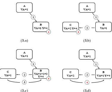
Panel 3.a diagrams a simple trade relationship in which country A produces 1 USD of intermediate inputs, which are used by B to produce 4 USD of local final goods. In this case, both KWW and our own bilateral decomposition classify (in components2and2arespectively)
the exports from A to B as ‘domestic VA in intermediate exports absorbed by direct importers’. In panel 3.b we now assume that B performs only a partial processing stage (worth 1 USD of VA) before sending the intermediate products to C, which assembles and consumes the final goods. The 1 USD of domestic VA exported by A is now absorbed in a third country (C), not the bilateral importer (B). This is correctly traced in our bilateral breakdown, as the A-B trade flow is allocated to component2c(i.e. ‘domestic VA in intermediate exports absorbed by third countries as local
final goods’). In KWW’s breakdown, however, it would be recorded by the term VABACYCC
and improperly classified as domestic VA of country A absorbed by the direct importer C, since in this case only B directly imports from A. Indeed the BAC, being part of the global inverse
Leontief matrix, accounts for all the possible ways in which the intermediate inputs of country A contribute to final goods produced in C, not only those directly imported by C.
In the example diagrammed in Figure 3.c, the intermediate products are processed in two subsequent production stages in B and C, then returned to B for a final stage before serving final demand. The very first shipment from A to B is correctly classified as ‘domestic VA in intermediate exports absorbed by direct importers’ both in KWW and in our own decomposition. But only our decomposition correctly recognizes that the domestic VA is absorbed by direct importers as local final goods only after additional processing stages abroad (2c). This also indicates the differences
B VA=3 Y=4 A
VA=1
1
4
(3.a)
C VA=2 Y=4
B VA=1 A
VA=1
1
2
4
(3.b)
C VA=1
B VA=1+1=2
Y=4 A
VA=1
1
2
4
3
(3.c)
C VA=2
B VA=1 Y=4 A
VA=1 1
2
4
[image:13.595.110.487.258.568.2](3.d)
and 3.c.
Scheme 3.d differs from 3.c only in that the final assembly stage is performed in C rather than B, which is still the country of final destination. As regards country A, B is both the direct importer and the final demand absorber, so its exports to B should be considered as domestic VA absorbed by a direct importer, which is how they are mapped in our decomposition (in item3c),
whereas in KWW’s method they are allocated to third countries’ absorption of domestic VA of exports.
The value added decomposition of bilateral trade flows offers useful information for valuing trade balances between countries, reconciling the gross export data with value added accounting. For instance, going back to the example in Figure 1, in case 1.a we see that the exports from A to B are generated by A’s demand for C’s final goods, since they are classified in item 4c
of equation (2) (i.e. ‘domestic VA in intermediate exports absorbed at home as final goods of a third country’). In example 1.b, instead, exports from A to C are classed under 4a (i.e.
‘domestic VA in intermediate exports absorbed at home as final goods of the bilateral importers’). This differentiation, which is not envisaged in KWW’s original framework, gives insights into the structure of international production and demand linkages, especially in dealing with the sort of complex production networks that prevail in the real world.
Our sink-based decomposition summarized by equation (2) differs substantially also from the one in Nagengast and Sterher (2016). In fact they classify as domestic value added absorbed by direct importers only that embedded in goods that do not leave this country again, assigning the remainder to the double counted component. In this way they do not take into account what we have classified in the2band3ccomponents, underestimating the domestic value added
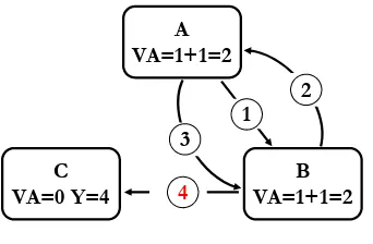
absorbed by direct importers. It means that, for instance, in the scheme 3.c and 3.d described above, the exports from country A to country B would be entirely classified as double counted in the decomposition of their bilateral flows. Also their definitions of the domestic value added finally absorbed at home and by third countries turn out to be imprecise, leading in this case to an overestimation of the domestic value added in exports. The scheme diagrammed in Figure 4 highlights this particular issue. In this case, two stages of production, each worth 1 USD of value added, are performed both in country A and B, before the final good being shipped from B to the destination market C. The total bilateral gross exports from A to B are equal to 4 USD, which consist of 2 USD of VA generated in A, 1 USD of VA generated in B and 1 USD of double counted VA, originated in the first stage of production in A and embedded in the second shipment from A to B. In Nagengast and Sterher (2016) this 1 USD of double counted items would be assigned to the domestic value added of A absorbed by third country C, overestimating this component.9
This
9
This overestimation stems from the double use of the global inverse Leontief matrix in some of the terms of the decomposition of Nagengast and Sterher (2016). In fact in the exam-ple of Figure 4, the domestic value added absorbed in third countries would be calculated as
VABAAAABBBBYBC (both in sink and source-based methodology). SinceBAAaccounts for all
the possible ways in which the intermediate inputs of country A contribute to the production in A, VABAA encompasses the entire value added of A generated both in the first and the second
stage of production. Then theVABAAmatrix should be applied only to the second export flow to
B, in order to extract A’s value added following the sink-based logic. Instead, since they account the B’s gross output necessary for the production of the final good exported to C through the
BBBmatrix, they are recording both the first and the second stage of production in B and hence
drawback applies both to their sink and source-based decompositions. This inaccuracy in defining some of the items entails that neither methodology proposed by Nagengast and Sterher (2016) can retrieve the entire domestic value added exported by a country summing the corresponding items across the bilateral flows. On the contrary both our sink-based decomposition and source-based breakdown, shown below, meet this requirement.
C VA=0 Y=4
B VA=1+1=2 A
VA=1+1=2 1
2 3
[image:15.595.214.385.189.301.2]4
Figure 4:
Domestic value added and double counting with final destination in third
countries
Figure 4 can be also used to point out another relevant issue of KWW’s methodology and of its bilateral version by Wang et al.(2013): the erroneous classification of part of the foreign value added in exports (i.e. the exclusion of items 9a and 9b of equation (2) from the foreign
value added). KKW’s classification fail to record the VA originated in the upstream stages of the production process by the country that exports to the market of final destination (i.e. countryr). We can make this point clearer by referring again to the scheme in figure 4. The 1 USD of value added produced by B in the second production phase should be considered as FVA in country A’s re-exports to B (i.e. the flow worth 3 USD), but in KWW’s classification this is recorded as double counted, as B is not the market of final destination. Instead braking down A’s exports according to equation (2) this component produced by B is correctly classified as foreign value added (within term9a).
Source-based breakdown of bilateral exports
The source-based decomposition of bilateral exports from countrysto countryrcan be expressed as follows:
uNEsr=
1a*
Vs(I−Ass)−1Ysr
+Vs(I−Ass)−1Asr(I−Arr)−1
"G
1b*
Xj6=r
ArjBjsYsr+
1c*
G
X
j6=r
Arj
G
X
k6=s,r
BjsYsk
#
[image:15.595.91.453.653.725.2]+Vs(I−Ass)−1Asr(I−Arr)−1
"
2a*
Yrr +
2b*
G
X
j6=r
ArjBjrYrr+
2c*
G
X
j6=r
Arj
G
X
k6=s,r
BjkYkk
#
+Vs(I−Ass)−1Asr(I−Arr)−1
"XG
3a*
j6=r,s
Yrj+
3b*
G
X
j6=r
Arj
G
X
l6=s,r
BjrYrl
+
3c*
G
X
j6=r
Arj
G
X
k6=s,r
BjkYkr+
3d*
G
X
j6=r
Arj
G
X
k6=s,r,l G
X
l6=s,r
BjkYkl
#
+Vs(I−Ass)−1Asr(I−Arr)−1
"
4a*
Yrs +
4b*
G
X
j6=r
ArjBjrYrs+
4c*
G
X
j6=r
Arj
G
X
k6=s,r
BjkYks
#
+
5*
Vs(I−Ass)−1Asr(I−Arr)−1
G
X
j6=r
ArjBjsYss
+
6*
Vs(I−Ass)−1
G
X
t6=s
AstBtsEsr
+
G
X
t6=s
Vt(I−Att)−1Ats(I−Ass)−1
"
7*
Ysr+
8*
Asr(I−Arr)−1Yrr
#
+
9a*
G
X
t6=s
Vt(I−Att)−1Ats(I−Ass)−1Asr(I−Arr)−1
G
X
j6=r
Yrj
+
9b*
G
X
t6=s
Vt(I−Att)−1Ats(I−Ass)−1Asr(I−Arr)−1
G
X
j6=r
Arj G X k G X l
BjkYkl
+
G
X
t6=s
Vt(I−Att)−1
" G
9c*
Xj6=t,s
AtjBjsEsr+
9d*
Ats(I−Ass)
G
X
t6=s
AstBtsEsr
#
(3)
We can define the items above as:
1a* domestic value added (VA) in final good exports directly absorbed by bilateral importers; 1b* domestic VA in intermediate exports absorbed by bilateral importers as domestic final
goods after additional processing stages;
1c* domestic VA in intermediate exports absorbed by third countries as domestic final goods
after additional processing stages;
2a* domestic VA in intermediate exports absorbed by direct importers as local final goods; 2b* domestic VA in intermediate exports absorbed by direct importers as local final goods only
after further processing stages;
3a* domestic VA in intermediate exports absorbed by third countries as final goods from direct
bilateral importers;
3b* domestic VA in intermediate exports absorbed by third countries as final goods from direct
bilateral importers only after further processing stages;
3c* domestic VA in intermediate exports absorbed by direct importers as final goods from third
countries;
3d* domestic VA in intermediate exports absorbed by third countries as final goods from other
third countries;
4a* domestic VA in intermediate exports absorbed at home as final goods of the bilateral
importers;
4b* domestic VA in intermediate exports absorbed at home as final goods of the bilateral
importers after further processing stages;
4c* domestic VA in intermediate exports absorbed at home as final goods of a third country; 5* domestic VA in intermediate exports absorbed at home as domestic final goods;
6* double-counted intermediate exports originally produced at home; 7* foreign VA in exports of final goods;
8* foreign VA in exports of intermediate goods directly absorbed by the importing countryr; 9a* and 9b* foreign VA in exports of intermediate goods re-exported byr;
9c* and 9d* double-counted intermediate exports originally produced abroad.
As for the sink-based decomposition, the enumeration of the items here above recalls the original KWW components. However while for the domestic content (terms1a*to 6*), the
correspondent KWW’s items can be obtained as a simple summation over the importing countries
r,10
this property does not hold for the foreign content part. At the level of the single exporter terms 7* to 9d* differ from those proposed in the sink-based decomposition of equation (2)
because the notions of FVA and FDC in KWW are defined at world level (not at country level like the DVA and the DDC). The source base classification of FVA and FDC of equation (3) follow a similar logic.11
However while in the source-based approach a certain item is recorded as FVA the first time that it is re-exported by a foreign country (and as FDC in all the other re-exports), in the sink-based framework all the FVA is accounted the last time that it is embedded in a export flow. Since the first re-exporter may not coincide with the last one, also the source-based indicators of foreign content and the sink-based ones usually differ when computed at the level of the exporting country. However both the approach account a given item as FVA only once in world trade flows. It means that aggregating at the world level the FVA and FDC components of equation (2) and (3) we obtain exactly the same measures. In section 2.3 we present an alternative approach to classify the foreign double counted from the perspective of the exporting country that leads to a unique measure of FVA and FDC both in a sink-based framework and in a source-based one.
10
A formal proof is available upon request. 11
Another feature of the source-based decomposition in (3) is that it identifies separately the domestic value added directly absorbed by the bilateral partner (terms 1a* and 2a*), i. e.
crossing just the border between the two countries, from the domestic value added absorbed by the bilateral partner only after further processing stages abroad or at home (terms1b*,2b*and 3c*). As we show in the empirical application presented in section 3.2, this is key to measure
global value chain related trade, defined as goods and services crossing more than one border, both at the bilateral and at the aggregate level.
This is also one the main feature that differentiates our methodology from the one proposed by Wang et al. (2013). Their decomposition does not allow to single out the goods that never leave the direct importing country since: i)the domestic value added in exports of final goods is measured through a sink-based accounting (i.e. VsBssYsr);ii) it does not identify intermediate
goods absorbed by the bilateral importer without additional processing stages abroad (notice that the term 2a* is only part of the correspondent component in Wang et al. (2013), Vs(I− Ass)−1A
srBrrYrr). More in general Wang et al. (2013) use different approaches (sink and
source) to single out the different components, so that their methodology suffers from internal inconsistency. This makes the items of the decomposition not comparable with each other. Since the trade in intermediaries and that in final goods are treated in different ways it could be tricky also to use their methodology to compare the value added structure of two (or more) distinct trade flows, as in the analysis of bilateral trade balances.12
2.3
An alternative breakdown of the foreign content of
ex-ports
As already mentioned, in equations (2) and (3) FVA and FDC are defined referring to world trade flows.13
It means that a certain item is considered as VA only the first (or the last) time it crosses a foreign border, while all the other times it is classified as double counted, even in the exports of different countries. On the other hand, the items produced domestically are considered as double counted only when they cross the same (national) border more than once.
The world perspective used to define the FVA and the FDC makes these measures partic-ularly unsatisfactory when analyzing the exports of a given country. Indeed this may make sense only in the breakdown of total world trade,14
but in the breakdown of a country’s exports this distinction of FVA and FDC turns out to be totally arbitrary. Consider the following example: Italy imports intermediaries directly from Germany and indirectly from France; according to a source-based approach the German VA is considered as FVA in Italian exports while the French
12
Indeed in a recent paper Wang et al. (2016) themselves adopt our source-based decomposition of equation (3).
13
This approach is adopted by all the other contributions in the literature that consider the dis-tinction between FVA and FDC, including Koopman et al. (2014), Wang et al. (2013), Nagengast and Sterher (2016) and Johnson (2017).
14
VA is classified as FDC, even if the two components contribute in very a similar way to the value embedded in Italian exports.15
From the perspective of the exporting country, we are usually interested in measuring the share of exports that can be traced back to the domestic GDP and the share that corresponds to the foreign one, independently from the number of upstream or downstream production stages that separate the exporter from the country of origin and/or the market of final destination. To this aim we need a notion of foreign double counting that follow the same logic adopted for the domestic double counting: we want to exclude from the FVA only the items that cross the same (domestic) border more than once.
Building on this intuition, we have developed a new sink-based decomposition of FVA and FDC and new source-based one defined according to the perspective of the exporting country.
The FVA in bilateral exports from countrysto countryrbased on a sink-based approach can be expressed as follows:
FVAsinksr=
7
G
X
t6=s
VtBtsYsr+
8
G
X
t6=s
VtBtsAsr(I−Arr)−1Yrr
+
9a
G
X
t6=s
VtBtsAsr(I−Arr)−1
G
X
j6=r
Yrj
+
9b
G
X
t6=s
VtBtsAsr(I−Arr)−1
G
X
j6=r
Arj
G
X
k6=s G
X
l
b
Bs✄
jkYkl
+
9b’
G
X
t6=s
VtBtsAsr(I−Arr)−1
G
X
j6=r
ArjBbs✄
jsYss (4)
The corresponding double counted component originated in foreign countries is the fol-lowing:
FDCsinksr=
9c
G
X
t6=s
VtBtsAsr(I−Arr)−1
G
X
j6=r
ArjBbs✄
jsEs∗ (5)
where the enumeration of the items recall that of equation (2) since they have similar interpreta-tion, however only the terms7and 8are exactly the same.
As in equation (2) the use of Bbs✄ ≡(I−A✄s)−1 allows us to take into account the entire
foreign value added in exports ofs, excluding only the trade flows that are re-exported more than once by the countrysitself. In particular in equation (4) the FVA is recorded the last time that it leaves the national borders, in line with the sink-based approach. Also in this case it is possible to derive a source-based counterpart of the decomposition of bilateral flows, in which the value
15
added is recorded in the first shipment from countrys.16
FVAsourcesr =
7*
G
X
t6=s
VtBbs✄
tsYsr
+
8*
G
X
t6=s
VtBbs✄
tsAsr(I−Arr)−1Yrr
+
9a*
G
X
t6=s
VtBbs✄
tsAsr(I−Arr)−1 G
X
j6=r
Yrj
+
9b*
G
X
t6=s
VtBbsts✄ Asr(I−Arr)−1
G
X
j6=r
Arj
G
X
k G
X
l
BjkYkl (6)
FDCsourcesr=
9c*
G
X
t6=s
VtBts
G
X
j6=t,s
AsjBbs✄
jsEsr (7)
Both the decompositions of the foreign components are completely consistent with each other when we sum across all destination markets (i.e. they produce the same values of FVA
and FDC for the aggregated exports of a country,
G
P
r6=s
FVAsinksr =
G
P
r6=s
FVAsourcesr). Thus
this new approach leads to a single measure of FVA (and FDC) at the country level. These new indicators can be used also to address other interesting empirical questions: which is the portion of a country’s GDP that is embedded into the exports of another country? How this is related to the markets of final destination?
2.4
The decomposition at the bilateral sector level
Our bilateral decompositions can be easily extended to the sectoral level.17
In particular, we focus on three different decompositions: i) by sector of origin of the value added, either domestic or foreign,ii) by sector of exports (the only one considered in the work of Wang et al., 2013) and iii) by sector of final absorption. To get a decomposition by sectors of origin, it is necessary to substitute in equation (2) or (3) the Vs and Vt vectors with Vbs and Vbt, the N×N diagonal matrices with the direct value added coefficients along the principal diagonal and zeros elsewhere. Instead, the decomposition by sectors of exports is obtained simply by substituting VsBss and VtBts withV\sBss andV\tBts, theN×N diagonal matrices with the value added shares in final
production along the principal diagonal and zeros elsewhere, as defined in Appendix A. Finally the
16
Again we use an enumeration that recalls the one assigned in the source-based decomposition in (3), even if all the corresponding terms differ in the two decompositions.
17
decomposition by sectors of final absorption is obtained by replacing the vectors of final demand, for instance for countryaandb,Yab, withYbab, theN×N diagonal matrices with country’sb
de-mand for final goods produced inaalong the principal diagonal and zeros elsewhere.18
Therefore, depending on the particular empirical application, it will be possible to choose the appropriate bilateral sectoral decomposition. These decompositions can also be combined: in order to measure simultaneously the value added embedded in a bilateral trade flow in a particular sector of origin destined for a particular sector of absorption, it is sufficient to use at the same timeVb andYb in
equation (2) or (3).
3
Two empirical applications
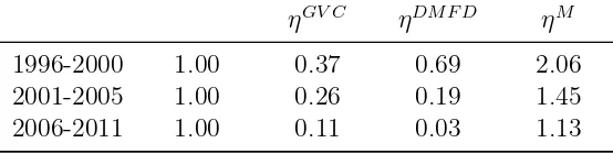
We use the OECD Trade in Value Added ICIO Tables (TiVA-ICIO, see OECD-WTO, 2012) and the World Input-Output Database (WIOD, see Dietzenbacher et al. 2013, Timmer et al. 2015) to show two different ways of exploiting the value added decompositions of bilateral trade. The first application follows the sink-based approach and focuses on the eight largest world exports, tracing their domestic VA in exports from direct importers to final demand. The second follows the source-based approach and derives a new measure of the share of GVC-related trade in order to determine how its evolution since the mid-1990s has affected the long-run relationship between global demand and world trade. Matlab codes for the sink and source-based decompositions are available upon request, both for WIOD and TiVA, as well as those to reproduce the empirical applications in the next sessions. A Stata command implementing the methods described in this paper is also available. It can be installed from within Stata by typingnet install icio, from(http://www.econometrics.it/stata).19
3.1
Major exporters’ forward connections
The decomposition of bilateral export flows provides useful information on the downstream struc-ture of the production networks in which a country is involved. In particular, in this section we investigate the channels through which the world top exporters reach the markets of final destination. We split the domestic value added in exports (DVA) into a share that is directly exported to the country of ultimate absorption and a share of DVA that passes through one or more intermediate countries before reaching the final markets. For each exporter and region of final destination we identify the five most important intermediate importers.
Thus, for this exercise, the sink-based decomposition presented in equation (2) is better suited, since it accounts the value added the very last time it crosses the national borders, which is the export flow more closely related with the market of ultimate absorption.20
The exercise is
18
See Appendix A for the derivation ofVb andYb. The matrixVBd is obtained in the same way.
19
Notice that the command cannot be downloaded from the website but just directly installed through the Stata software.
20
carried on with TiVA data for 2011.
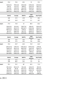
We consider the eight largest global exporters (China, US, Germany, Japan, UK, France, Italy and Korea) and four main regions of destination (Europe, NAFTA, Latin America and Asia-Pacific), in addition to the world total. First, for each exporter we measure the relative weight of different markets as ultimate destinations of domestic VA, as compared to their relative shares in terms of gross exports. Table 1 shows that the two distributions are very similar to each other only for the US and China. Regarding the Euro Area, Asia-Pacific is a much more relevant destination in terms of value added compared to gross exports, while the opposite holds for exports among European countries, since a relevant share of trade flows within the so called Factory Europe (Baldwin and Lopez-Gonzales, 2013) is made of intermediate goods that cross many times national borders. Japan and Korea show the most significant divergence between the gross and the value added composition of exports. In particular, the share of value added exports towards Asia-Pacific is 10 percentage points lower than the one computed in gross terms.
Then, for each country of exports and region of destination, we single out 1) the share of domestic VA that is directly absorbed by the bilateral importer, that by definition also belongs to the region of destination, and 2) the share of domestic VA that passes through one or more inter-mediate countries (within or outside the region of destination) before reaching the final market. Regarding the latter, we also identify which are the first five intermediate countries that directly import from the country of origin.
China’s role as a final hub within the Factory Asia is confirmed looking at Japanese and Korean exports. Around 20% (17%) of the domestic VA produced in Korea and finally absorbed in North America (Europe) is embedded in Korean bilateral exports to China. In the case of Japan the share of domestic VA embedded in exports to China is particularly high for products destined for the Latin-American market (more than 17% of the total). Also a relevant share of Japanese and Korean value added that is consumed in the Asia-Pacific region passes through China.
To some extent, a similar role is played by Germany within Factory Europe. Germany delivers a relevant share of “made in Italy” and “made in France” especially toward more distant markets: around 4.5% of Italian and French value added destined to the Asia-Pacific market reaches that region passing through Germany.
China is not only the hub of Factory Asia, but also of the overall global production. In fact, despite the geographical distance, China is the first intermediate importers for Germany, the second for the US, the third for Italy and the fourth for France. In particular, it turns out that a relevant share of European productions destined for the North-American market passes through China.
ITALY World Europe NAFTA Latin
America Asia Pacific GERMANY World Europe NAFTA
Latin
America Asia Pacific % of total gross exports 100 62.1 9.9 2.2 12.7 % of total gross exports 100 62.7 10.3 2 17 % total DVA absorbed in foreign markets 100 57.1 12.3 2.7 13.8 % total DVA absorbed in foreign markets 100 57.1 13 2.5 17
% of DVA absorbed by the direct importer 78.5 81.7 71.8 76.8 69.6 % of DVA absorbed by the country of direct import 75.6 79.4 69.1 72 72.1
% of DVA 1st intermediate importer DEU (3.4) DEU (3.2) CHN (3.7) DEU (3.3) DEU (4.5) % of DVA 1st intermediate importer CHN (2.5) FRA (1.8) CHN (5.8) CHN (4.4) CHN (4.3)
% of DVA 2nd intermediate importer FRA (2.1) FRA (2.1) DEU (3.7) CHN (2.4) CHN (3.2) % of DVA 2nd intermediate importer FRA (2) ITA (1.5) GBR (2) USA (2.3) FRA (1.7)
% of DVA 3rd intermediate importer CHN (1.6) ESP (1.3) MEX (2) FRA (2) FRA (2.3) % of DVA 3rd intermediate importer ITA (1.6) CZE (1.4) USA (1.9) FRA (2.2) CHE (1.7)
% of DVA 4th intermediate importer ESP (1.2) CHE (0.9) FRA (1.9) USA (1.7) CHE (1.6) % of DVA 4th intermediate importer CHE (1.4) AUT (1.4) MEX (1.9) ITA (1.8) USA (1.5)
% of DVA 5th intermediate importer CHE (1) POL (0.9) GBR (1.6) ESP (1.4) USA (1.5) % of DVA 5th intermediate importer GBR (1.4) POL (1.3) FRA (1.7) CHE (1.4) KOR (1.5)
FRANCE World Europe NAFTA Latin
America Asia Pacific UNITED STATES World Europe NAFTA
Latin
America Asia Pacific % of total gross exports 100 61.8 9.7 1.8 13.5 % of total gross exports 100 27.2 23.9 6.1 30.2 % total DVA absorbed in foreign markets 100 57.2 12.1 2.2 14.2 % total DVA absorbed in foreign markets 100 26.9 24.7 6.1 28.7
% of DVA absorbed by the direct importer 78.2 81.3 71.9 71.9 69.6 % of DVA absorbed by the country of direct import 77.5 73.9 72 88.1 81.2
% of DVA 1st intermediate importer DEU (3.7) DEU (3.5) DEU (3.9) DEU (4.2) DEU (4.6) % of DVA 1st intermediate importer CAN (2.6) IRL (3.4) CAN (7.6) MEX (2) CHN (2.6)
% of DVA 2nd intermediate importer ITA (1.8) ESP (2) CHN (3.7) CHN (2.8) CHN (3.1) % of DVA 2nd intermediate importer CHN (2.5) DEU (2.7) MEX (6.7) CHN (1.6) KOR (1.7)
% of DVA 3rd intermediate importer ESP (1.7) ITA (1.8) GBR (2.3) ITA (2.2) ITA (1.9) % of DVA 3rd intermediate importer MEX (2.2) CHN (2.2) CHN (3) CAN (0.7) SGP (1.4)
% of DVA 4th intermediate importer CHN (1.5) BEL (1.4) ITA (1.8) ESP (2.2) GBR (1.8) % of DVA 4th intermediate importer IRL (1.7) GBR (1.6) IRL (1.5) KOR (0.7) TWN (1.1)
% of DVA 5th intermediate importer GBR (1.5) GBR (1.2) USA (1.3) USA (2) USA (1.5) % of DVA 5th intermediate importer DEU (1.3) FRA (1.3) KOR (0.8) BRA (0.6) CAN (1.1)
JAPAN World Europe NAFTA Latin
America Asia Pacific KOREA World Europe NAFTA
Latin
America Asia Pacific % of total gross exports 100 12.6 18.9 1.5 57.5 % of total gross exports 100 13.1 14.2 2.9 58.9 % total DVA absorbed in foreign markets 100 16.1 23.7 2.5 45.4 % total DVA absorbed in foreign markets 100 17.1 20.1 3.8 45.4
% of DVA absorbed by the country of direct
import 71.5 57.9 69.8 56.5 77.9 % of DVA absorbed by the country of direct import 73.5 59.7 64.5 73.5 81.9 % of DVA 1st intermediate importer CHN (9.7) CHN (13.8) CHN (12.9) CHN (17.2) CHN (6.2) % of DVA 1st intermediate importer CHN (12.6) CHN (17) CHN (20.3) CHN (14.4) CHN (8)
% of DVA 2nd intermediate importer KOR (3.4) KOR (3.7) KOR (2.9) KOR (5.5) KOR (3.4) % of DVA 2nd intermediate importer TWN (1.4) DEU (2.3) MEX (2.9) USA (1.9) TWN (1.7)
% of DVA 3rd intermediate importer TWN (2.8) DEU (3.1) TWN (2.6) USA (4) TWN (3.2) % of DVA 3rd intermediate importer USA (1.2) USA (1.7) USA (1.6) MEX (1.1) JPN (1.1)
% of DVA 4th intermediate importer USA (1.7) TWN (2.5) MEX (2) TWN (3) THA (1.9) % of DVA 4th intermediate importer JPN (1.1) RUS (1.2) TWN (1.6) TWN (1) SGP (0.9)
% of DVA 5th intermediate importer THA (1.7) USA (2.4) USA (2) THA (2.1) MYS (1.5) % of DVA 5th intermediate importer DEU (0.8) TWN (1.2) CAN (1.2) JPN (0.7) MYS (0.8)
CHINA World Europe NAFTA Latin
America Asia Pacific UNITED KINGDOM World Europe NAFTA
Latin
America Asia Pacific % of total gross exports 100 23.5 26 3.5 35 % of total gross exports 100 53.5 17.7 1.4 17 % total DVA absorbed in foreign markets 100 24.3 25.7 3.8 32.8 % total DVA absorbed in foreign markets 100 48.1 20.1 1.9 18
% of DVA absorbed by the country of direct
import 82.9 78 85.9 85 83.3 % of DVA absorbed by the country of direct import 76.1 76.7 80 64.1 71.9 % of DVA 1st intermediate importer USA (1.8) DEU (2.2) MEX (2.6) USA (2.8) KOR (2.4) % of DVA 1st intermediate importer DEU (3.2) DEU (3.7) IRL (2.8) USA (4.7) DEU (3)
% of DVA 2nd intermediate importer KOR (1.7) USA (1.8) USA (1.7) KOR (1.7) JPN (1.6) % of DVA 2nd intermediate importer IRL (2.6) IRL (3) DEU (2.1) DEU (4.3) SGP (2.2)
% of DVA 3rd intermediate importer JPN (1.1) FRA (1.3) KOR (1.1) 0 (1.4) USA (1.6) % of DVA 3rd intermediate importer FRA (1.4) BEL (1.6) CHN (1.9) CHN (2.7) USA (2.2)
% of DVA 4th intermediate importer DEU (1) ITA (1.1) CAN (1.1) MEX (1.2) TWN (1.5) % of DVA 4th intermediate importe