Magnetotactic Bacteria Algorithm for Function Optimization

Magnetotactic

Bacteria Algorithm

for Function

Optimization

Hongwei Mo

1

, Lifang Xu

2

1

Automation College, Harbin Engineering University, Harbin, China; 2Engineering Training Center, Harbin Engineering University, Harbin, China

Email: [email protected]

ABSTRACT

Magnetotactic bacteria is a kind of polyphyletic group of prokaryotes with the characteristics of magnetotaxis that make them orient and swim along geomagnetic field lines. A magnetotactic bacteria optimization algorithm(MBOA) inspired by the characteristics of magnetotactic bacteria is researched in the paper. Experiment results show that the MBOA is effective in function optimization problems and has good and competitive performance compared with the other clas-sical optimization algorithms.

Keywords: Magnetotactic bacteria optimization algorithm; Function optimization; Nature inspired computing

1.

Introduction

Learning from life system, people have developed many nature inspired computing(NIC) methods to solve com-plicated optimization computation problems in recent decades. There has been a considerable attention paid for employing algorithms inspired from natural processes and/or events in order to solve optimization problems. For example, genetic algorithms(GAs) which was first introduced by Holland are now a standard optimization tool in engineering. Since 1980s, more and more NIC algorithms were developed following GAs, including Ant Colony Optimization(ACO)[1] and Particle Swarm Optimization(PSO)[2], Immune Algorithm(IA)[3], Ar-tificial Bee Colony(ABC)[4], Bacterial Chemotaxis Al-gorithm[5], Biogeography based Optimization[6] and so on.

Since many studies were carried out with inspirations from ecological phenomena for developing optimization techniques, we still pay attention to find new inspiration source. ‘No free lunch theorem’ had told us that there is no universal algorithm which can be better over all possible problems. So it is necessary for us to develop new algorithms for problem solving. Tayarani proposed a magnetic optimization algorithm which is based on the principle of particles’ interaction in magnetic optimiza-tion [7]. In nature, there is a kind of polyphyletic group of prokaryotes that can orient and swim along magnetic field lines. They are called magnetotactic bacteria (MTBs) [8]. A striking property of MTBs is their ability to orient and propel themselves along geomagnetic field lines

(magnetotaxis) in the earth magnetic field. Propelled by their flagella, the bacteria migrate in a net downward direction, following the declination of the field lines of the earth, toward oxygen-poor regions with advantages for survival.

In[9], we have proposed a new algorithm called mag-netotactic bacteria optimization algorithm (MBOA) in-spired by the distinct behavior of MTBs. It had been tested on some standard benchmarks and compared with some optimization algorithms, and it shows good per-formance in solving some optimization problems of standard functions. In this paper, MBOA is researched in further.

The remainder of this paper is organized as follows: Section 2 describes the basic procedure of MBOA. In Section 3, experiments on 14 standard functions optimi-zation and analysis are provided. Finally, the conclusions are drawn in Section 4 .

2.

MBOA

2.1.

Principles of MBOA

In magnetotactic bacteria, magnetosomes play impor-tant role in regulating the movement of MTBs. The magnetic field lines bend in some of the magnetosomes to minimize their magnetostatic energy[11], whereas in others their direction differs slightly from that of the chain axis. In fact, the MTBs have evolved to be adap-tive to the magnetic field. Based on the biology know-ledge, we know that one kind of MTBs has multiple cells with chains of magnetosomes. Only those MTBs with magnetosomes in their cells which can make magnetic field lines bend in some of the magnetosomes to minim-ize their magnetostatic energy can survive in nature. Each magnetosome can produce moment[11]. The MTBs with multi-cell need to produce magnetosome moments with which can minimize their magnetostatic energy. We can consider such a process as an optimization one.

When the MBA runs to solve a problem, it corres-ponds to the process of producing magnetosomes to be adaptive to magnetic field. It needs to regulate the mo-ments of each magnetosome, just like producing feasible solutions. MBOA obtains the optimal solution by regu-lating the moments of cells continually.

Consider a problem solving inspired by MTBs, the minimal magnetostatic energy is looked as optimal solu-tion. The multiple cells are looked as feasible solutions. The magnetosomes in each cell can be looked as the fea-tures of a candidate solution. The moment of a magneto-some corresponds to feature value.

2.2.

Procedures of MBOA

Considering a chain of magnetosomes as a cylinder of infinite length in a magnetic field B, its energy

E

_a of the bacterial, moment can be estimated as follows.

θ

cos

MB

B

M

E

m

=

−

⋅

=

−

(1)

where

θ

is the angle between M and B.

According to[9], the interaction energy between two dipoles from different magnetosome chains in a MTB with multi cells is:

3 ,

1













+

+

=

mD

nD

D

E

nm (2)

where

n

,

m

=

0

,

1

,

2

...

are the number of magnetosomes of two cells,

d

is the distance between neighbor centers in a chain.

Suppose that the interaction energy between two cells in a MTB as follows:

m n m

n

E

E

E

)

_,

(

2

1

+

=

(3)

where

E

_n

,

E

_mare the energy of two cells, respectively. If two cells have the same number of magnetosomes, that is

n

=

m

, and suppose

E

_n

=

E

_m, then we have

m n m

n

E

E

,

=

, (4)

The total procedure of MBOA is described as follows: 1: Generate initial cells population

C

nand set con-stant

λ

,

ρ

,

a

.

2: While (

t

<

MaxGenerat

ion

)

3: calculate cost of each cell

4: normalize cost to calculate magnetic field

B

5: for

i

=

1

:

n

6: for

j

=

1

:

n

7: If

i

≠

j

8: calculate the distance

D

9: If

D

>

r

10: calculate interaction energy

E

of two cells 11: else

12:

E

=

rand

(

1

,

p

)

*

R

13: end 14: end

15: for

i

=

1

:

n

16: calculate moment

M

of each cell

17 regulate the moment of each cell by

M

18: end

19: calculate the cost

J

of each cell, rank the cells, re-place some proportional cells by randomly produced moments.

20: rank the cells and find the optimal solution 21: end while

The procedure of MBA is described as follows in de-tail:

Step 1: All of the moments of magnetosomes in cell population (for t=0) are initialized randomly between upper and lower limit of feature value.

In step 4: The

i

th magnetic field value

f

_iis normalized as follows:

)

min(

)

max(

)

min(

i i

i i

i

f

f

f

f

f

−

−

=

(5)

n

ρ

λ +

=

i

i

f

B

(6)

where

λ

and

ρ

are constant.

In step 8: we define the distance between two cells as:

∑

=

=

n

j i

j i

d

D

1 ,

, /U (7)

Suppose that

x

_i,k

,

x

_j,k

∈

[

−

L

,

U

]

are the

k

th feature value (moment) of

x



_i

,

x



_j, respectively.

n

is the population size.

−

L

and

U

are the lower limit and upper limit of feature value. Then

D

can be defined as the following function.

∑

=

−

=

p

k

k j k i j

i

U

x

x

p

x

x

D

1

, ,

1

)

,

(





(8)

In step 9,

r

=

a

∗

(

U

/

2

)

*

p

, where

a

is a distance threshold constant.

In step 10, suppose that Mi =(m1,m2,...,mp) ,

n

i

=

1

,...,

is the

i

th moment of magnetosome of a cell. Assume the interaction energy

E

between two cells as Equation (9).

3 ,

2

1













+

=

mD

D

E

i j (9)

According to Equation (1), and for simplification, suppose

cos

θ

=1, then we get

i j i i

B

E

M

=

, (10)

So we have the ways of regulating moments of mag-netosomes in a cell (individual) as follows:

t i t

i t

i

x

M

x

=

−1

+

(11)

where

x

_it

,

x

_it−1 are the

i

th moment of the

i

th indi-vidual(cell) in

t

generation.

M

_it is the moment of corresponding individual in

t

generation.

In step 19: after the regulation, the solutions are sorted according to their costs in ascending. The last half of cells is replaced by the following way:

R

m

rand

m

rand

x

i

=

λ

∗

((

(

1

,

)

−

1

)

∗

(

1

,

))

/

(12)

In general, the generation number is set as the stop-ping condition. At last, find the optimal result and output the result.

3.

Experiment Results and Analysis

3.1.

Problem Definition

Global numerical optimization problems are frequently arisen in almost every field of engineering design, ap-plied sciences, molecular biology and other scientific applications. Without loss of generality, the global mi-nimization problem can be formalized as a pair

(

S

,

f

)

, where

S

⊆

R

D is a bounded set on

R

D and

R

S

f

:

→

is a D-dimensional real value function. The problem is to find a point

X

*

∈

S

such that

)

(

X

*

f

is the global minimum on S. More specifically, it is required to find an

X

*

∈

S

such that

)

(

)

(

:

f

X

*

f

X

S

X

∈

≤

∀

(13)

where f does not need to be continuous but it must be bounded.

3.2.

Parameter Settings

In all experiments in this section, all algorithms are the basic ones without any improvement. The values of the common parameters used in each algorithm such as pop-ulation size and total evaluation number were chosen to be the same. Population size was 50 and the maximum evaluation number was 500 for all functions. The other specific parameters of algorithms are given below[12]:

GA Settings: Single point crossover operation with the rate of 0.8 was employed. Mutation rate was 0.01. Sto-chastic uniform sampling technique was our selection method.

DE Settings: F is a real constant which affects the dif-ferential variation between two solutions and set to 0.5 in our experiments. Value of crossover rate was chosen to be 0.9.

MBOA: For MBOA, we only need to set

λ

and

ρ

to decide magnetic field. In our experiments,

λ

=

0

.

5

,

0001

.

0

=

ρ

.

3.3.

Experiment Results

In order to characterize the type of problems for which the algorithm is suitable and test the performance of MBOA, we used 14 benchmark problems in order to comparison the performance of these algorithms. This set is large enough to include many different kinds of prob-lems such as unimodal(U), multimodal(M), regular, ir-regular, separable(S), non-separable(N) and multidimen-sional. Initial range, formulation, the dimensions(D), parameters setting and characteristics(C) of these prob-lems are listed in Table 1. The minimal values of Easom and Dropwave are -1. The minimal value of all the other functions is 0. The formulations of benchmark functions are shown in Table 2.

The compared results of the MAB with GA, PSO, DE on a large set of functions are listed in Table 3 and Ta-ble 4. Each of the experiments in this section was re-peated 30 times with different random seeds and the mean best values produced by the algorithms have been recorded. In order to make comparison clear, the values below ₁₀−12_{are assumed to be 0.}

Table 1. Characteristic of benchmark functions

No. Function Range D C

1 Step [-100, 100] 30 US

2 Sphere [-100, 100] 30 US

3 SumSquares [-10, 10] 30 US

4 Quartic [-1.28, 1.28] 30 US

5 Easom [-100, 100] 2 UN

6 Schwefel1.2 [-100, 100] 30 UN

7 Zakharov [-5, 10] 10 UN

8 Powell [-4, 5] 24 UN

9 Rotatedhyper [-65.536,65.536] 30 UN

10 Rastrigin [-5.12, 5,12] 30 MS

11 Branin [ 5,10] [0,15]− × 2 MS

12 Dropwave [-5.12,5.12 1] 2 MS

13 Schaffer [-100, 100] 2 MN

14 Griewank [-600, 600] 30 MN

Table 2. Benchmark function formulations

No. Formulations

1

(

)

2

1

( ) ni i 0.5 f x =

∑

₌ _x + _

2 2

1

( ) ni i f x =

∑

₌ x

3 2

1

( ) n_i i

f x =

∑

₌ix

4 f x( )=

∑

ni=₁ixi4+random[0,1)

5 f x( )= −cos( ) cos(x₁ x₂) exp( (− x₁−π)2−(x₂−π) )2

6 ( ) n₁( i _{1 j})2

i j

f x =

∑ ∑

_{= =} x

7 2 2 4

1 1 1

( ) n _i ( n 0.5 _i) ( n 0.5 _i)

i i i

f x =

∑

₌x +

∑

₌ ix +

∑

₌ ix

8

/ 2 2 4

4 3 4 2 4 1 4 4 2 4 1

1 4 4 3 4

( ) ( 10 ) 5( ) ( )

10( )

n k

i i i i i i

i

i i

f x x x x x x x

x x − − − − − = − = + + − + − + −

∑

9

∑ ∑

= =      = n i i j j x x f 1 2 1 ) (

10 2

1

( ) n [ _i 10 cos(2 _i) 10

i

f x =

∑

₌ x − πx +

11 _{2 1}2 ₁ 2 ₁

2

5.1 5 1

( ) ( 6) 10(1 ) cos 10

4 8

f x x x x x

π π π

= − + − + − + 12 2 ) ( 2 / 1 ) 12 cos( 1 ) , ( ₂ 2 2 1 2 2 2 2

1 _{+ +}

+ + − = x x x x x x f 13

2 2 2

1 2

2 2 2

1 2

sin ( ) 0.5 ( ) 0.5

(1 0.001( )) x x f x x x + − = + + +

14 ( ) 1 ₁ 2 ₁cos 1

4000 n n _i i i i x

f x x

i = =   = − _{ }+  

∑

∏

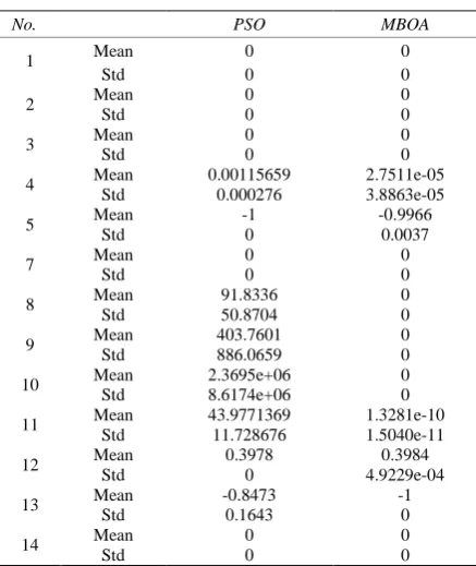
Because of space limit, we separate experiment results to two sets as shown in Table 3 and Table 4, respective-ly. Statistical results of 30 runs obtained by GA, DE MBOA are shown in Table 3 and those of PSO and MBOA are shown in Table 4, where Mean: Mean of the Best Values, Std: Standard Deviation of the Best Values.

Table 3. Comparison results of GA, DE and MBOA

No. GA DE MBOA

1 Mean 78.2333 0 0

Std 41.1563 0 0

2 Mean 91.1986 0 0

Std 36.4409 0 0

3 Mean 0.4881 0 0

Std 1.1443 0 0

4 Mean _Std 0.2670 _0.2237 0.006891 _0.00148 2.7511e-05 _3.8863e-05

5 Mean -0.6413 -1 -0.9966

Std 0.4614 0 0.0037

6 Mean 2.4527e+04 18324.1 0

Std 6.4361e+03 3022.165 0

7 Mean 0.2301 0 0

Std 0.6375 0 0

8 Mean 2.5631 0.059135 0

Std 1.6810 0.02199 0

9 Mean 395.4911 1.9523e-09 0

Std 182.5482 2.3682e-09 0

10 Mean 0 98.21781 1.3281e-10

Std 0 7.976648 1.5040e-11

Std 0.0127 0 4.9229e-04 12 Mean _Std -0.9793 _0.0561 -1 ₀ -1 ₀

13 Mean 0.0010 0 0

Std 0.0031 0 0

14 Mean 0.7959 0 0

Std 0.4205 0 0

[image:5.595.314.518.74.664.2]

As seen from Tables 3 and Tables 4, there are 8 func-tions with 30 variables. MBOA outperforms all the other algorithms on 4(Quartic, Powell, Rotatedhyper, Rastrigin) and has the same performance on 1(Matyas) with GA, DE, PSO. It has the same performance on 5 (Step, Sphere, Sumsquares, Schaffer, Griewank) with DE, PSO, GA has the worst performance on these functions. It is better than GA on Step, Sphere, Schaffer, Griewank, Easom, Schwefel1.2, but is worse than PSO, DE on Ea-som, Branin. It is better than GA, PSO on Zakhavov. And it has the same performance as DE on Dropwave. It is better than DE, PSO on Rastrigin and worse than GA. It is better than GA but worse than PSO, DE on Branin. In total, it is better than PSO on 6, GA on 12, DE on 5 of these 14 functions. So, MBOA has better performance than GA on these functions and is competitive with PSO, DE on these functions.

Table 4. Comparison results of PSO and MBOA

No. PSO MBOA

1 Mean 0 0

Std 0 0

2 Mean 0 0

Std 0 0

3 Mean _Std 0 ₀ 0 ₀

4 Mean 0.00115659 2.7511e-05

Std 0.000276 3.8863e-05

5 Mean -1 -0.9966

Std 0 0.0037

7 Mean 0 0

Std 0 0

8 Mean 91.8336 0

Std 50.8704 0

9 Mean 403.7601 0

Std 886.0659 0

10 Mean 2.3695e+06 0

Std 8.6174e+06 0

11 Mean 43.9771369 1.3281e-10

Std 11.728676 1.5040e-11

12 Mean _Std 0.3978 _{0 4.9229e-04} 0.3984

13 Mean -0.8473 -1

Std 0.1643 0

14 Mean 0 0

Std 0 0

0 50 100 150 200 250 300 350 400 450 500 0

0.5 1 1.5 2 2.5

3x 10

5

Generation

Co

s

t

Sphere

GA DE PSO MBOA

(a)

0 50 100 150 200 250 300 350 400 450 500 -1

-0.9 -0.8 -0.7 -0.6 -0.5 -0.4 -0.3 -0.2 -0.1 0

Generation

Co

st

Easom

GA DE PSO MBOA

(b)

0 50 100 150 200 250 300 350 400 450 500 0

100 200 300 400 500 600 700

Generation

Co

st

Rastrigin

GA DE PSO MBOA

(c)

0 50 100 150 200 250 300 350 400 450 500 0

500 1000 1500 2000 2500 3000

Generation

Co

st

Griewank

GA DE PSO MBOA

(d)

Figure 1. Comparison on convergence of the four algorithms.

[image:5.595.62.281.371.631.2]

The four functions have difference characteristics as shown in Table1. We can see that MBOA converges much faster than PSO, DE and GA.

4.

Conclusions

In this paper, a new nature inspired computing method- Magnetotactic Bacteria Optimization Algorithm is re-searched. It adopts the principles of energy and moment of magnetosomes in magnetotactic bacteria to produce optimal solution for engineering problems. It has simple procedure and is easy to implement. The experimental results show that it is effective in solving optimization problems and is competitive with the compared classical algorithms PSO and DE. And it converges faster than PSO, DE and GA. It shows competitive performance with some classical algorithms, such as GA, DE, PSO. In future, it needs to be analyzed in theory and improved its performance for solving more complex problems.

5.

Acknowledgements

This work is supported by the National Natural Science Foundation of China under Grant No.61075113, the Ex-cellent Youth Foundation of Heilongjiang Province of ChinaNo.JC201212 and the Fundamental Research Funds for the Central Universities No.HEUCFZ1209.

REFERENCES

[1] L. N. De Castro, F. J. Von Zuben. “Learning and Opti-mization Using the Clonal Selection Principle,” IEEE Trans. on Evolutionary Computation, Vol.6,No.3,

pp.239–251, 2002.

[2] M. Dorigo, V. Manianiezzo, A. Colorni. “The Ant Sys-tem: Optimization by a Colony of Cooperating Agents,”

IEEE Trans.Sys. Man and Cybernetics, Vol.26, No.1,pp. 1-13.

[3] R. E. Dunin-Borkowski, M. R. McCartney, R. B. Frankel, D. A. Bazylinski, M. Posfai, P. R Buseck. “Magnetic

Mi-crostructure of Magnetotactic Bacteria by Electron Holo-graphy,” Science, Vol. 282, 1998,

pp.1868-1870.

[4] D. Karaboga, B. Akay. “A Comparative Study of Artifi-cial Bee Colony Algorithm,” Applied Mathematics and Computation, Vol 214, No.1,2009, pp.108–132.

[5] J. Kennedy, R. Eberhart. Particle swarm optimization.

IEEE Int Conf on Neural Networks. Piscataway, NJ,

1995,pp.1942-1948

[6] S. Müeller, J. Marchetto, S. Airaghi, P. Koumoutsakos. “Optimization Based on Bacterial Chemotaxis,” IEEE Trans on Evolutionary Computation, Vol.6, No.1,2002, pp.16-29.

[7] A. P. Philipse, D. Maas. “Magnetic Colloids from Mag-netotactic Bacteria: Chain Formation and Colloidal Sta-bility,” Langmuir, Vol.18, 2002,pp.9977-9984.

[8] D. Simon. “Biogeography-based Optimization,” IEEE Trans on Evolutionary Computation, Vol. 12, 2008,

pp.702-713

[9] Mo Hongwei, “Research on Magnetotactic Bacteria Op-timization Algorithm,” The Fifth International Confe-rence on Advanced Computational Intelli-gence,Nanjing,Oct,2012,pp.417-422.

[10] M. H. N. Tayarani, T. Akbarzadeh. “Magnetic Optimiza-tion Algorithms A New Synthesis,” in Proc. of IEEE Congress on Evolutionary Computation. Hong Kong, China, 1-6,June,2008,pp. 2659-2665.

[11] M. Winklhofer, L. G. Abraçado, A. F. Davila, C. N. Keim, H. G. Lins de Barros. P. “Magnetic Optimization in A Multicellular Magnetotactic Organism,” Biophysical

Journal