Proceedings of the 55th Annual Meeting of the Association for Computational Linguistics, pages 1591–1600 Vancouver, Canada, July 30 - August 4, 2017. c2017 Association for Computational Linguistics Proceedings of the 55th Annual Meeting of the Association for Computational Linguistics, pages 1591–1600
Vancouver, Canada, July 30 - August 4, 2017. c2017 Association for Computational Linguistics
Neural Modeling of Multi-Predicate Interactions for
Japanese Predicate Argument Structure Analysis
Hiroki Ouchi1,2 Hiroyuki Shindo1,2 Yuji Matsumoto1,2 1 Nara Institute of Science and Technology
2 RIKEN Center for Advanced Intelligence Project (AIP)
{ouchi.hiroki.nt6, shindo, matsu }@is.naist.jp
Abstract
The performance of Japanese predicate ar-gument structure (PAS) analysis has im-proved in recent years thanks to the joint modeling of interactions between multi-ple predicates. However, this approach re-lies heavily on syntactic information pre-dicted by parsers, and suffers from error propagation. To remedy this problem, we introduce a model that uses grid-type re-current neural networks. The proposed model automatically induces features sen-sitive tomulti-predicate interactionsfrom the word sequence information of a sen-tence. Experiments on the NAIST Text Corpus demonstrate that without syntactic information, our model outperforms previ-ous syntax-dependent models.
1 Introduction
Predicate argument structure (PAS) analysis is a basic semantic analysis task, in which systems are required to identify the semantic units of a sen-tence, such as who did what to whom. In pro-drop languages such as Japanese, Chinese and Italian, arguments are often omitted in text, and such argument omission is regarded as one of the most problematic issues facing PAS analy-sis (Iida and Poesio,2011;Sasano and Kurohashi,
2011;Hangyo et al.,2013).
In response to the argument omission prob-lem, in Japanese PAS analysis, a joint model of the interactions between multiple predicates has been gaining popularity and achieved the state-of-the-art results (Ouchi et al., 2015; Shibata et al.,
2016). This approach is based on the linguistic in-tuition that the predicates in a sentence are seman-tically related to each other, and capturing this re-lation can be useful for PAS analysis. In the
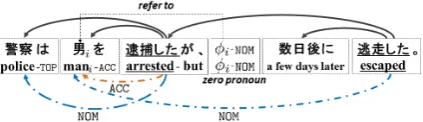
exam-Figure 1: Example of Japanese PAS. The upper edges denote dependency relations, and the lower edges denote case arguments. “NOM” and “ACC” denote the nominative and accusative arguments, respectively. “ϕi” is azero pronoun, referring to
theantecedent“男i(mani)”.
ple sentence in Figure1, the word “男i(mani)” is
the accusative argument of the predicate “逮捕し た(arrested)” and is shared by the other predicate
“逃走した(escaped)” as its nominative argument.
Considering the semantic relation between “逮捕 した(arrested)” and “逃走した(escaped)”, we
in-tuitively know that the person arrested by someone is likely to be the escaper. That is, information about one predicate-argument relation could help to identify another predicate-argument relation.
However, to model such multi-predicate inter-actions, the joint approach in the previous stud-ies relstud-ies heavily on syntactic information, such as part-of-speech (POS) tags and dependency re-lations predicted by POS taggers and syntactic parsers. Consequently, it suffers from error propa-gation caused by pipeline processing.
To remedy this problem, we propose a neural model which automatically induces features sen-sitive to multi-predicate interactions exclusively from the word sequence information of a sentence. The proposed model takes as input all predicates and their argument candidates in a sentence at a time, and captures the interactions using grid-type recurrent neural networks (Grid-RNN) with-out syntactic information.
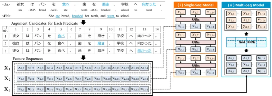
[image:1.595.312.524.223.284.2]Figure 2: Overview of neural models: (i)single-sequenceand (ii)multi-sequencemodels.
In this paper, we first introduce a basic model that uses RNNs. This model independently es-timates the arguments of each predicate without considering multi-predicate interactions (Sec. 3). Then, extending this model, we propose a neural model that uses Grid-RNNs (Sec. 4).
Performing experiments on the NAIST Text Corpus (Iida et al., 2007), we demonstrate that even without syntactic information, our neu-ral models outperform previous syntax-dependent models (Imamura et al.,2009;Ouchi et al.,2015). In particular, the neural model using Grid-RNNs achieved the best result. This suggests that the proposed grid-type neural architecture effec-tively captures multi-predicate interactions and contributes to performance improvements.1
2 Japanese Predicate Argument Structure Analysis
2.1 Task Description
In Japanese PAS analysis, arguments are identi-fied that each fulfills one of the three major case roles,nominative(NOM),accusative(ACC) and da-tive(DAT) cases, for each predicate. Arguments can be divided into the following three categories according to the positions relative to their predi-cates (Hayashibe et al.,2011;Ouchi et al.,2015):
Dep: Arguments that have direct syntactic depen-dency on the predicate.
Zero: Arguments referred to by zero pronouns within the same sentence that have no direct syntactic dependency on the predicate.
Inter-Zero: Arguments referred to by zero pro-nouns outside of the same sentence.
1Our source code is publicly available at
https://github.com/hiroki13/neural-pasa-system
For example, in Figure1, the nominative argument “警察 (police)” for the predicate “逮捕した
(ar-rested)” is regarded as a Dep argument, because the argument has a direct syntactic dependency on the predicate. By contrast, the nominative ar-gument “男i (mani)” for the predicate “逃走し た(escaped)” is regarded as aZeroargument, be-cause the argument has no direct syntactic depen-dency on the predicate.
In this paper, we focus on the analysis for these intra-sentential arguments, i.e., Dep and
Zero. In order to identify inter-sentential argu-ments (Inter-Zero), a much broader space must be searched (e.g., the whole document), resulting in a much more complicated analysis than intra-sentential arguments.2 Owing to this
complica-tion,Ouchi et al.(2015) and Shibata et al.(2016) focused exclusively on intra-sentential argument analysis. Following this trend, we also restrict our focus to intra-sentential argument analysis.
2.2 Challenging Problem
Arguments are often omitted in Japanese sen-tences. In Figure1,ϕirepresents the omitted argu-ment, called thezero pronoun. This zero pronoun
ϕi refers to “男i (mani)”. In Japanese PAS anal-ysis, when an argument of the target predicate is omitted, we have to identify the antecedent of the omitted argument (i.e., theZeroargument).
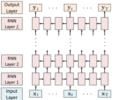
Figure 3: Overall architecture of the single-sequence model. This model consists of three components: (i) Input Layer, (ii) RNN Layer and (iii) Output Layer.
cate “逮捕した (arrested)”, the nominative
argu-ment is “警察(police)”. This argument is easily
identified by relying on the syntactic dependency. By contrast, because the nominative argument “男
i(mani)” has no syntactic dependency on its pred-icate “逃走した(escaped)”, we must rely on other
information to identify the zero argument.
As a solution to this problem, we exploit two kinds of information: (i) the context of the en-tire sentence, and (ii) multi-predicate interactions. For the former, we introduce single-sequence model that induces context-sensitive representa-tions from a sequence of argument candidates of a predicate. For the latter, we introduce multi-sequence model that induces predicate-sensitive representations from multiple sequences of argu-ment candidates of all predicates in a sentence (shown in Figure2).
3 Single-Sequence Model
The single-sequence model exploits stacked bidi-rectional RNNs (Bi-RNN) (Schuster and Paliwal,
1997; Graves et al., 2005, 2013; Zhou and Xu,
2015). Figure 3 shows the overall architecture, which consists of the following three components:
Input Layer: Map each word to a feature vector representation.
RNN Layer: Produce high-level feature vectors using Bi-RNNs.
[image:3.595.89.275.62.226.2]Output Layer: Compute the probability of each case label for each word using the softmax function.
[image:3.595.322.511.62.223.2]Figure 4: Example of feature extraction. The un-derlined word is the target predicate. From the sentence “彼女はパンを食べた。(She ate bread.)”, three types of features are extracted for the target predicate “食べた(ate)”.
Figure 5: Example of the process of creating a fea-ture vector. The extracted feafea-tures are mapped to each vector, and all the vectors are concatenated into one feature vector.
In the following subsections, we describe each of these three components in detail.
3.1 Input Layer
Given an input sentence w1:T = (w1,· · · , wT)
and a predicate p, each word wt is mapped to a feature representationxt, which is the
concatena-tion (⊕) of three types of vectors:
xt=xargt ⊕xpredt ⊕xmarkt (1)
where each vector is based on the following atomic features inspired byZhou and Xu(2015):
ARG: Word index of each word.
PRED: Word index of the target predicate and the words around the predicate.
[image:3.595.323.513.312.432.2]Figure 4 presents an example of the atomic fea-tures. For theARGfeature, we extract a word index
xword ∈ V for each word. Similarly, for thePRED feature, we extract each word indexxword for the
C words taking the target predicate at the center,
whereCdenotes the window size. TheMARK fea-ture xmark ∈ {0,1} is a binary value that repre-sents whether or not the word is the predicate.
Then, using feature indices, we extract feature vector representations from each embedding ma-trix. Figure 5 shows the process of creating the feature vector x1 for the word w1 “彼女 (she)”.
We set two embedding matrices: (i) a word em-bedding matrix Eword ∈ Rdword×|V|, and (ii)
a mark embedding matrix Emark ∈ Rdmark×2.
From each embedding matrix, we extract the cor-responding column vectors and concatenate them as a feature vectorxtbased on Eq.1.
Each feature vector xtis multiplied with a pa-rameter matrixWx:
h(0)t =Wxxt (2)
The vectorh(0)t is given to the first RNN layer as
input.
3.2 RNN Layer
In the RNN layers, feature vectors are updated re-currently using Bi-RNNs. Bi-RNNs process an input sequence in a left-to-right manner for odd-numbered layers and in a right-to-left manner for even-numbered layers. By stacking these layers, we can construct the deeper network structures.
Stacked Bi-RNNs consist of L layers, and the
hidden state in the layerℓ ∈ (1,· · · , L)is
calcu-lated as follows:
h(tℓ)=
{
g(ℓ)(h(ℓ−1)
t , h
(ℓ)
t−1) (ℓ= odd)
g(ℓ)(h(ℓ−1)
t , h
(ℓ)
t+1) (ℓ= even)
(3)
Both of the odd- and even-numbered layers re-ceiveh(tℓ−1), thet-th hidden state of theℓ−1layer,
as the first input of the functiong(ℓ), which is an
arbitrary function3. For the second input ofg(ℓ),
odd-numbered layers receiveh(tℓ−)1, whereas
even-numbered layers receiveh(tℓ+1) . By calculating the
hidden states until theL-th layer, we obtain a
hid-den state sequenceh(1:TL) = (h1(L),· · · ,h(TL)).
Us-ing each vectorh(tL), we calculate the probability
of case labels for each word in the output layer. 3In this work, we used the Gated Recurrent Unit (GRU) (Cho et al.,2014) as the functiong(ℓ).
3.3 Output Layer
For the output layer, multi-class classification is performed using the softmax function:
yt=softmax(Wyh(tL))
whereh(tL)denotes a vector representation propa-gated from the last RNN layer (Fig3). Each ele-ment ofytis a probability value corresponding to each label. The label with the maximum probabil-ity among them is output as a result. In this work, we set five labels:NOM,ACC,DAT,PRED,null. PREDis the label for the predicate, andnull de-notes a word that does not fulfill any case role.
4 Multi-Sequence Model
Whereas the single-sequence model assumes inde-pendence between predicates, the multi-sequence model assumes multi-predicate interactions. To capture such interactions between all predi-cates in a sentence, we extend the single-sequence model to the multi-single-sequence model us-ing Grid-RNNs (Graves and Schmidhuber, 2009;
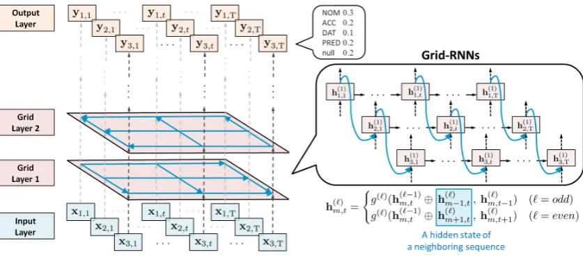
Kalchbrenner et al.,2016). Figure6 presents the overall architecture for the multi-sequence model, which consists of three components:
Input Layer: Map words to M sequences of feature vectors forM predicates.
Grid Layer: Update the hidden states over dif-ferent sequences using Grid-RNNs.
Output Layer: Compute the probability of each case label for each word using the soft-max function.
In the following subsections, we describe these three components in detail.
4.1 Input Layer
The multi-sequence model takes as input a sen-tence w1:T = (w1,· · · , wT) and all predicates
{pm}M1 in the sentence. For each predicate pm,
the input layer creates a sequence of feature vec-tors Xm = (xm,1,· · · ,xm,T) by mapping each
input word wt to a feature vector xm,t based on Eq1. That is, forM predicates, M sequences of
feature vectors{Xm}M1 are created.
Then, using Eq. 2, each feature vector xm,t is mapped toh(0)m,t, and a feature sequence is created for a predicatepm, i.e.,H(0)m = (h(0)m,1,· · ·,h
(0)
m,T).
Consequently, forMpredicates, we obtainM
Figure 6: Overall architecture of the multi-sequence model: an example of three sequences.
4.2 Grid Layer
Inter-Sequence Connections
For the grid layers, we use Grid-RNNs to propa-gate the feature information over the different se-quences (inter-sequence connections). The fig-ure on the right in Figfig-ure 6 shows the first grid layer. The hidden state is recurrently calculated from the upper-left (m = 1, t = 1) to the
lower-right (m=M, t= T).
Formally, in theℓ-th layer, the hidden stateh(m,tℓ)
is calculated as follows:
h(m,tℓ)=
{
g(ℓ)(h(m,tℓ−1)⊕hm(ℓ)−1,t,hm,t(ℓ)−1) (ℓ= odd)
g(ℓ)(h(m,tℓ−1)⊕hm(ℓ)+1,t,h(m,tℓ)+1) (ℓ= even)
This equation is similar to Eq. 3. The main differ-ence is that the hidden state of a neighboring se-quence, h(m−ℓ) 1,t (or h(mℓ)+1,t), is concatenated (⊕) with the hidden state of the previous (ℓ−1) layer, h(m,tℓ−1), and is taken as input of the functiong(ℓ).
In the figure on the right in Figure6, the blue curved lines represent the inter-sequence connec-tions. Taking as input the hidden states of neigh-boring sequences, the network propagates feature information over multiple sequences (i.e., pred-icates). By calculating the hidden states until the L-th layer, we obtain M sequences of the
hidden states, i.e., {H(mL)}M1 , in which H(mL) =
(h(m,L)1,· · ·,h(m,L)T).
Residual Connections
As more layers are stacked, it becomes more dif-ficult to learn the model parameters, owing to various challenges such as the vanishing gradi-ent problem (Pascanu et al., 2013). In this work,
we integrate residual connections (He et al.,2015;
Wu et al., 2016) with our networks to form con-nections between layers. Specifically, the in-put vector h(m,tℓ−1) of the ℓ-th layer is added to
the output vector h(m,tℓ). Residual connections
can also be applied to the single-sequence model. Thus, we can perform experiments on both models with/without residual connections.
4.3 Output Layer
As with the single-sequence model, we use the softmax function to calculate the probability of the case labels of each wordwtfor each predicatepm:
ym,t =softmax(Wyh(m,tL))
whereh(m,tL) is a hidden state vector calculated in
the last grid layer.
5 Related Work
5.1 Japanese PAS Analysis Approaches
Existing approaches to Japanese PAS analy-sis are divided into two categories: (i) the
pointwise approach and (ii) the joint approach. The pointwise approach involves estimating the score of each argument candidate for one pred-icate, and then selecting the argument can-didate with the maximum score as an argu-ment (Taira et al., 2008; Imamura et al., 2009;
2011; Ouchi et al., 2015; Shibata et al., 2016). Compared with the pointwise approach, the joint approach achieves better results.
5.2 Multi-Predicate Interactions
Ouchi et al.(2015) reported that it is beneficial to Japanese PAS analysis to capture the interactions between all predicates in a sentence. This is based on the linguistic intuition that the predicates in a sentence are semantically related to each other, and that the information regarding this semantic relation can be useful for PAS analysis.
Similarly, in semantic role labeling (SRL),
Yang and Zong (2014) reported that their rerank-ing model, which captures the multi-predicate in-teractions, is effective for the English constituent-based SRL task (Carreras and M`arquez, 2005). Taking this a step further, we propose a neu-ral architecture that effectively models the multi-predicate interactions.
5.3 Neural Approaches Japanese PAS
In recent years, several attempts have been made to apply neural networks to Japanese PAS anal-ysis (Shibata et al., 2016; Iida et al., 2016)4. In Shibata et al. (2016), a feed-forward neural net-work is used for the score calculation part of the joint model proposed by Ouchi et al. (2015). In Iida et al. (2016), multi-column convolutional neural networks are used for the zero anaphora res-olution task.
Both models exploit syntactic and selectional preference information as the atomic features of neural networks. Overall, the use of neural net-works has resulted in advantageous performance levels, mitigating the cost of manually designing combination features. In this work, we demon-strate that even without such syntactic informa-tion, our neural models can realize comparable performance exclusively using the word sequence information of a sentence.
English SRL
Some neural models have achieved high perfor-mance without syntactic information in English SRL. Collobert et al. (2011) and Zhou and Xu
(2015) worked on the English constituent-based 4These previous studies used unpublished datasets and evaluated the performance with different experimental set-tings. Consequently, we cannot compare their models with ours.
SRL task (Carreras and M`arquez, 2005) using neural networks. In Collobert et al.(2011), their model exploited a convolutional neural network and achieved a 74.15% F-measure without syn-tactic information. In Zhou and Xu (2015), their model exploited bidirectional RNNs with linear-chain conditional random fields (CRFs) and achieved the state-of-the-art result, an 81.07% F-measure. Our models should be regarded as an extension of their model.
The main differences between Zhou and Xu
(2015) and our work are: (i) constituent-based vs dependency-based argument identification and (ii) the multi-predicate consideration. For the constituent-based SRL,Zhou and Xu(2015) used CRFs to capture the IOB label dependencies, be-cause systems are required to identify the spans
of arguments for each predicate. By contrast, for Japanese dependency-based PAS analysis, we re-placed the CRFs with the softmax function, be-cause in Japanese, arguments are rarely adjacent to each other.5 Furthermore, whereas the model
described in Zhou and Xu (2015) predicts argu-ments for each predicate independently, our multi-sequence model jointly predicts arguments for all predicates in a sentence concurrently by consider-ing the multi-predicate interactions.
6 Experiments
6.1 Experimental Settings Dataset
We used the NAIST Text Corpus 1.5, which con-sists of 40,000 sentences from Japanese news-papers (Iida et al., 2007). For the experiments, we adopted standard data splits (Taira et al.,2008;
Imamura et al.,2009;Ouchi et al.,2015):
Train: Articles: Jan 1-11, Editorials: Jan-Aug
Dev: Articles: Jan 12-13, Editorials: Sept
Test: Articles: Jan 14-17, Editorials: Oct-Dec
We used the word boundaries annotated in the NAIST Text Corpus and the target predicates that have at least one argument in the same sentence. We did not use any external resources.
Learning
We trained the model parameters by minimizing
the cross-entropy loss function:
L(θ) =−∑ n
∑
t
logP(yt|xt) +λ
2||θ|| 2 (4)
where θ is a set of model parameters, and the
hyper-parameterλis the coefficient governing the
L2 weight decay.
Implementation Details
We implemented our neural models using a deep learning library, Theano (Bastien et al., 2012). The number of epochs was set at 50, and we re-ported the result of the test set in the epoch with the best F-measure from the development set. The parameters were optimized using the stochastic gradient descent method (SGD) via a mini-batch, whose size was selected from{2,4,8}. The
learn-ing rate was automatically adjusted uslearn-ing Adam (Kingma and Ba,2014). For the L2 weight decay, the hyper-parameterλin Eq. 4was selected from
{0.001,0.0005,0.0001}.
In the neural models, the number of the RNN and Grid layers were selected from {2,4,6,8}.
The window size C for the PRED feature (Sec.
3.1) was set at5. Words with a frequency of2or
more in the training set were mapped to each word index, and the remaining words were mapped to the unknown word index. The dimensionsdword anddmarkof the embeddings were set at32. In the single-sequence model, the parameters of GRUs were set at32×32. In the multi-sequence model,
the parameters of GRUs related to the input val-ues were set at64×32, and the remaining were
set at32×32. The initial values of all parameters
were sampled according to a uniform distribution from[−√ √6
row+col, √
6
√
row+col], where row andcol are the number of rows and columns of each ma-trix, respectively.
Baseline Models
We compared our models to existing models in previous works (Sec.5.1) that use the NAIST Text Corpus 1.5. As a baseline for the pointwise ap-proach, we used the pointwise model6proposed in Imamura et al. (2009). In addition, as a baseline for the joint approach, we used the model pro-posed in Ouchi et al. (2015). These models ex-ploit gold annotations in the NAIST Text Corpus as POS tags and dependency relations.
6We compared the results of the model reimplemented by Ouchi et al.(2015).
Dep Zero All
Imamura+ 09 85.06 41.65 78.15
Ouchi+ 15 86.07 44.09 79.23
Single-Seq 88.10 46.10 81.15
Multi-Seq 88.17† 47.12† 81.42†
Table 1: F-measures in the test set. Single-Seqis the single-sequence model, andMulti-Seq
is the multi-sequence model. Imamura+ 09 is the model inImamura et al.(2009) reimplemented by Ouchi et al. (2015), and Ouchi+ 15 is the
ALL-Cases Joint Model in Ouchi et al. (2015).
The mark†denotes the significantly better results with the significance level p < 0.05, comparing
Single-SeqandMulti-Seq.
6.2 Results
Neural Models vs Baseline Models
Table 1 presents F-measures from our neural se-quence models with eight RNN or Grid layers and the baseline models on the test set. For the significant test, we used the bootstrap resampling method. According to all metrics, both the
single-(Single-Seq) and multi-sequence models (
Multi-Seq) outperformed the baseline models. This confirms that our neural models realize high per-formance, even without syntactic information, by learning contextual information effective for PAS analysis from the word sequence of the sentence.
In particular, for zero arguments (Zero), our models achieved a considerable improvement compared to the joint model inOuchi et al.(2015). Specifically, the single-sequence model improved by approximately 2.0 points, and the multi-sequence model by approximately 3.0 points ac-cording to the F-measure. These results suggest that modeling the context of the entire sentence us-ing RNNs are beneficial to Japanese PAS analysis, particularly to zero argument identification.
Effects of Multiple Predicate Consideration
As Table 1 shows, the multi-sequence model significantly outperformed the single-sequence model in terms of the F-measure overall (81.42% vs 81.15%). These results demonstrate that the grid-type neural architecture can effectively cap-ture multi-predicate interactions by connecting the sequences of the argument candidates for all pred-icates in a sentence.
dif-Single-Seq Multi-Seq
L +res. −res. +res. −res.
2
Dep 87.34 87.10 87.43 87.73 Zero 47.98 47.90 47.66 46.93
All 80.62 80.24 80.71 80.68
4 ZeroDep 87.2750.43 87.4150.83 87.6048.10 87.0948.58
All 80.92 80.99 80.99 80.59
6 ZeroDep 87.7348.81 87.1149.51 88.0448.98 87.3948.91
All 81.05 80.63 81.19 80.68
8 ZeroDep 87.9847.40 87.2348.38 87.6549.34 87.0748.23
[image:8.595.77.287.63.259.2]All 81.31 80.33 81.33 80.40
Table 2: Performance comparison for different numbers of layers on the development set in F-measures.Lis the number of the RNN or Grid
lay-ers. +res.or−res.indicates whether the model
has residual connections (+) or not (−).
ferent argument types, the multi-sequence model achieved slightly better results for direct depen-dency arguments (Dep) (88.10% vs 88.17%). In addition, for zero arguments (Zero), which have no syntactic dependency on their predicate, the multi-sequence model outperformed the single-multi-sequence model by approximately 1.0 point according to the F-measure (46.10% vs 47.12%). This shows that capturing multi-predicate interactions is particu-larly effective for zero arguments, which is con-sistent with the results inOuchi et al.(2015).
Effects of Network Depth
Table 2 presents F-measures from the neural se-quence models with different network depths and with/without residual connections. The perfor-mance tends to improve as the RNN or Grid layers get deeper with residual connections. In partic-ular, the two models with eight layers and resid-ual connections achieved considerable improve-ments of approximately 1.0 point according to the F-measure compared to models without residual connections. This means that residual connec-tions contribute to effective parameter learning of deeper models.
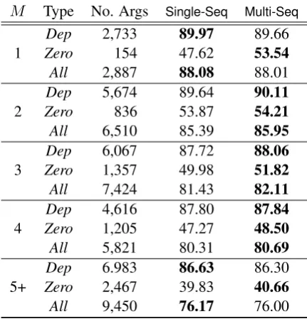
Effects of the Number of Predicates
Table 3 presents F-measures from the neural se-quence models with different numbers of predi-cates in a sentence. In Table 3, M denotes how
M Type No. Args Single-Seq Multi-Seq
1 ZeroDep 2,733154 89.9747.62 89.6653.54
All 2,887 88.08 88.01
2 ZeroDep 5,674836 89.6453.87 90.1154.21
All 6,510 85.39 85.95
3
Dep 6,067 87.72 88.06
Zero 1,357 49.98 51.82
All 7,424 81.43 82.11
4 ZeroDep 4,6161,205 87.8047.27 87.8448.50
All 5,821 80.31 80.69
5+
Dep 6.983 86.63 86.30
Zero 2,467 39.83 40.66
All 9,450 76.17 76.00
Table 3: Performance comparison for different numbers (M) of predicates in a sentence on the
test set in F-measures.
many predicates appear in a sentence. For exam-ple, the sentence in Figure1 includes two predi-cates, “arrested” and “escaped”, and thus in this exampleM = 2.
Overall, performance of both models gradu-ally deteriorated as the number of predicates in a sentence increased, because sentences that con-tain many predicates are complex and difficult to analyze. However, compared to the single-sequence model, the multi-single-sequence model sup-pressed performance degradation, especially for zero arguments (Zero). By contrast, for direct
dependency arguments (Dep), both models either
achieved almost equivalent performance or the single-sequence model outperformed the multi-sequence model. A Detailed investigation of the relation between the number of predicates in a sen-tence and the complexity of PAS analysis is an in-teresting line for future work.
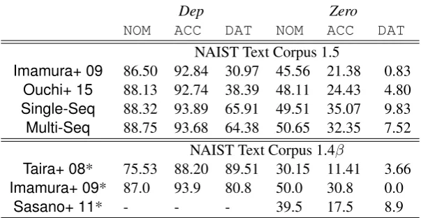
Comparison per Case Role
Table4shows F-measures for each case role. For reference, we show the results of the previous studies using the NAIST Text Corpus 1.4β with external resources as well.7
7The major difference between the NAIST Text Corpus 1.4βand 1.5 is the revision of the annotation criterion for the dative case (DAT) (corresponding to Japanese case marker “
[image:8.595.308.524.65.289.2]Dep Zero
NOM ACC DAT NOM ACC DAT
NAIST Text Corpus 1.5
Imamura+ 09 86.50 92.84 30.97 45.56 21.38 0.83
Ouchi+ 15 88.13 92.74 38.39 48.11 24.43 4.80
Single-Seq 88.32 93.89 65.91 49.51 35.07 9.83
Multi-Seq 88.75 93.68 64.38 50.65 32.35 7.52
NAIST Text Corpus 1.4β
Taira+ 08* 75.53 88.20 89.51 30.15 11.41 3.66
Imamura+ 09* 87.0 93.9 80.8 50.0 30.8 0.0
[image:9.595.148.450.65.221.2]Sasano+ 11* - - - 39.5 17.5 8.9
Table 4: Performance comparison for different case roles on the test set in F-measures. NOM,ACC or DATis the nominal, accusative or dative case, respectively. The asterisk (*) indicates that the model uses external resources.
Comparing the models using the NAIST Text Corpus 1.5, the single- and multi-sequence mod-els outperformed the baseline modmod-els according to all metrics. In particular, for the dative case, the two neural models achieved much higher results, by approximately 30 points. This suggests that al-though dative arguments appear infrequently com-pared with the other two case arguments, the neu-ral models can learn them robustly.
In addition, for zero arguments (Zero), the neural models achieved better results than the baseline models. In particular, for zero argu-ments of the nominative case (NOM), the multi-sequence model demonstrated a considerable im-provement of approximately 2.5 points accord-ing to the F-measure compared with the joint model inOuchi et al.(2015). To achieve high ac-curacy for the analysis of such zero arguments, it is necessary to capture long distance depen-dencies (Iida et al., 2005; Sasano and Kurohashi,
2011;Iida et al., 2015). Therefore, the improve-ments of the results suggest that the neural models effectively capture long distance dependencies us-ing RNNs that can encode the context of the entire sentence.
7 Conclusion
In this work, we introduced neural sequence mod-els that automatically induce effective feature rep-resentations from the word sequence information of a sentence for Japanese PAS analysis. The experiments on the NAIST Text Corpus demon-strated that the models realize high performance without the need for syntactic information. In par-ticular, our multi-sequence model improved the
performance ofzero argumentidentification, one of the problematic issues facing Japanese PAS analysis, by considering themulti-predicate inter-actionswith Grid-RNNs.
Because our neural models are applicable to SRL, applying our models for multilingual SRL tasks presents an interesting future research direc-tion. In addition, in this work, the model param-eters were learned without any external resources. In future work, we plan to explore effective meth-ods for exploiting large-scale unlabeled data to learn the neural models.
Acknowledgments
This work was partially supported by JST CREST Grant Number JPMJCR1513 and JSPS KAK-ENHI Grant Number 15K16053. We are grateful to the members of the NAIST Computational Lin-guistics Laboratory and the anonymous reviewers for their insightful comments.
References
Fr´ed´eric Bastien, Pascal Lamblin, Razvan Pascanu, James Bergstra, Ian J. Goodfellow, Arnaud Berg-eron, Nicolas Bouchard, and Yoshua Bengio. 2012. Theano: new features and speed improvements. Deep Learning and Unsupervised Feature Learning NIPS 2012 Workshop.
for statistical machine translation. InProceedings of EMNLP. pages 1724–1734.
Ronan Collobert, Jason Weston, Leon Bottou, Michael Karlen, Koray Kavukcuoglu, and Pavel Kuksa. 2011. Natural language processing (almost) from scratch. Journal of Machine Learning Research.
Alan Graves, Navdeep Jaitly, and Abdel-rahman Mo-hamed. 2013. Hybrid speech recognition with deep bidirectional LSTM. In Proceedings of Automatic Speech Recognition and Understanding (ASRU), 2013 IEEE Workshop.
Alex Graves, Santiago Fern´andez, and J¨urgen Schmid-huber. 2005. Bidirectional LSTM networks for im-proved phoneme classification and recognition. In Proceedings of International Conference on Artifi-cial Neural Networks. pages 799–804.
Alex Graves and J¨urgen Schmidhuber. 2009. Offline handwriting recognition with multidimensional re-current neural networks. In Proceedings of NIPS. pages 545–552.
Masatsugu Hangyo, Daisuke Kawahara, and Sadao Kurohashi. 2013. Japanese zero reference resolu-tion considering exophora and author/reader men-tions. InProceedings of EMNLP. pages 924–934.
Yuta Hayashibe, Mamoru Komachi, and Yuji Mat-sumoto. 2011. Japanese predicate argument struc-ture analysis exploiting argument position and type. InProceedings of IJCNLP. pages 201–209.
Kaiming He, Xiangyu Zhang, Shaoqing Ren, and Jian Sun. 2015. Deep residual learning for image recog-nition.arXiv preprint arXiv:1512.03385.
Ryu Iida, Kentaro Inui, and Yuji Matsumoto. 2005. Anaphora resolution by antecedent identification followed by anaphoricity determination. ACM Transactions on Asian Language Information Pro-cessing (TALIP)4(4):417–434.
Ryu Iida, Mamoru Komachi, Kentaro Inui, and Yuji Matsumoto. 2007. Annotating a Japanese text cor-pus with predicate-argument and coreference rela-tions. In Proceedings of the Linguistic Annotation Workshop. pages 132–139.
Ryu Iida and Massimo Poesio. 2011. A cross-lingual ILP solution to zero anaphora resolution. In Pro-ceedings of ACL-HLT. pages 804–813.
Ryu Iida, Kentaro Torisawa, Chikara Hashimoto, Jong-Hoon Oh, and Julien Kloetzer. 2015. Intra-sentential zero anaphora resolution using subject sharing recognition. In Proceedings of EMNLP. pages 2179–2189.
Ryu Iida, Kentaro Torisawa, Jong-Hoon Oh, Cana-sai Kruengkrai, and Julien Kloetzer. 2016. Intra-sentential subject zero anaphora resolution using multi-column convolutional neural network. In Pro-ceedings of EMNLP. pages 1244–1254.
Kenji Imamura, Kuniko Saito, and Tomoko Izumi. 2009. Discriminative approach to predicate-argument structure analysis with zero-anaphora res-olution. InProceedings of ACL-IJCNLP. pages 85– 88.
Nal Kalchbrenner, Ivo Danihelka, and Alex Graves. 2016. Grid long short-term memory. In Proceed-ings of ICLR.
D.P. Kingma and J. Ba. 2014. Adam: A method for stochastic optimization. arXiv preprint arXiv: 1412.6980.
Hiroki Ouchi, Hiroyuki Shindo, Kevin Duh, and Yuji Matsumoto. 2015. Joint case argument identifica-tion for Japanese predicate argument structure anal-ysis. In Proceedings of ACL-IJCNLP. pages 961– 970.
Razvan Pascanu, Tomas Mikolov, and Yoshua Bengio. 2013. On the difficulty of training recurrent neural networks. InProceedings of ICML.
Ryohei Sasano and Sadao Kurohashi. 2011. A dis-criminative approach to Japanese zero anaphora res-olution with large-scale lexicalized case frames. In Proceedings of IJCNLP. pages 758–766.
Mike Schuster and Kuldip K Paliwal. 1997. Bidirec-tional recurrent neural networks. IEEE Transactions on Signal Processingpages 2673–2681.
Tomohide Shibata, Daisuke Kawahara, and Sadao Kurohashi. 2016. Neural network-based model for Japanese predicate argument structure analysis. In Proceedings of ACL. pages 1235–1244.
Hirotoshi Taira, Sanae Fujita, and Masaaki Nagata. 2008. A Japanese predicate argument structure anal-ysis using decision lists. InProceedings of EMNLP. pages 523–532.
Yonghui Wu, Mike Schuster, Zhifeng Chen, Quoc V Le, Mohammad Norouzi, Wolfgang Macherey, Maxim Krikun, Yuan Cao, Qin Gao, Klaus Macherey, et al. 2016. Google’s neural ma-chine translation system: Bridging the gap between human and machine translation. arXiv preprint arXiv:1609.08144.
Haitong Yang and Chengqing Zong. 2014. Multi-predicate semantic role labeling. InProceedings of EMNLP. pages 363–373.
Katsumasa Yoshikawa, Masayuki Asahara, and Yuji Matsumoto. 2011. Jointly extracting Japanese predicate-argument relation with markov logic. In Proceedings of IJCNLP. pages 1125–1133.