Blind Phoneme Segmentation With Temporal Prediction Errors

Proceedings of the 55th Annual Meeting of the Association for Computational Linguistics- Student Research Workshop, pages 62–68 Vancouver, Canada, July 30 - August 4, 2017. c2017 Association for Computational Linguistics

Proceedings of the 55th Annual Meeting of the Association for Computational Linguistics- Student Research Workshop, pages 62–68 Vancouver, Canada, July 30 - August 4, 2017. c2017 Association for Computational Linguistics

Blind phoneme segmentation with temporal prediction errors

Paul Michel1∗ _{Okko Rasanen}2 _{Roland Thiolli`ere}3 _{Emmanuel Dupoux}3

1_{Carnegie Mellon University,}2_{Aalto University,}3_{LSCP / ENS / EHESS / CNRS}

[email protected], [email protected], [email protected], [email protected]

Abstract

Phonemic segmentation of speech is a crit-ical step of speech recognition systems. We propose a novel unsupervised algo-rithm based on sequence prediction mod-els such as Markov chains and recurrent neural networks. Our approach consists in analyzing the error profile of a model trained to predict speech features frame-by-frame. Specifically, we try to learn the dynamics of speech in the MFCC space and hypothesize boundaries from lo-cal maxima in the prediction error. We evaluate our system on the TIMIT dataset, with improvements over similar methods.

1 Introduction

One of the main difficulty of speech processing as opposed to text processing is the continuous, time-dependent nature of the signal. As a conse-quence, pre-segmentation of the speech signal into words or sub-words units such as phonemes, syl-lables or words is an essential first step of a variety of speech recognition tasks.

Segmentation in phonemes is useful for a num-ber of applications (annotation of speech for the purpose of phonetic analysis, computation of speech rate, keyword spotting, etc), and can be done in two ways. Supervised methods are based on an existing phoneme or word recognition sys-tem, which is used to decode the incoming speech into phonemes. Phonemes boundaries can then be extracted as a by-product of the alignment of the phoneme models with the speech. Unsuper-vised methods (also called blind segmentation) consist in finding phonemes boundaries using the acoustic signals only. Supervised methods depend

∗

This work was done when the author was an intern at LSCP / ENS / EHESS / CNRS

on the training of acoustic and language models, which requires access to large amounts of linguis-tic resources (annotated speech, phonelinguis-tic dictio-nary, text). Unsupervised methods do not require these resources and are therefore appropriate for so-called under-resourced languages, such as en-dangered languages, or languages without consis-tent orthographies.

We propose a blind phoneme segmentation method based on short term statistical properties of the speech signal. We designate peaks in the error curve of a model trained to predict speech frame by frame as potential boundaries. Three dif-ferent models are tested. The first is an approx-imated Markov model of the transition probabili-ties between categorical speech features. We then replace it by a recurrent neural network operating on the same categorical features. Finally, a recur-rent neural network is directly trained to predict the raw speech features. This last model is espe-cially interesting in that it couples our statistical approach with more common spectral transition based methods (Dusan and Rabiner(2006) for in-stance).

We first describe the various models used and the pre- and post-processing procedures, before presenting and discussing our results in the light of previous work.

2 Related work

Most previous work on blind phoneme segmenta-tion (Esposito and Aversano,2005;Estevan et al., 2007;Almpanidis and Kotropoulos, 2008; Rasa-nen et al., 2011; Khanagha et al., 2014; Hoang and Wang, 2015) has focused on the analysis of the rate of change in the spectral domain. The idea is to design robust acoustic features that are supposed to remain stable within a phoneme, and change when transitioning from one phoneme to

the next. The algorithm then define a measure of change, which is then used to detect phoneme boundaries.

Apart from this line of research, three main approaches have been explored. The first idea is to use short term statistical dependencies. In R¨as¨anen (2014), the idea was to first discretize the signal using a clustering algorithm and then compute discrete sequence statistics, over which a threshold can be defined. This is the idea that we follow in the current paper. The second approach is to use dynamic programming methods inspired by text segmentation (Wilber, 1988), in order to derive optimal segmentation (Qiao et al.,2008). In this line of research, however, the number of seg-ments is assumed to be known in advance, so this cannot count as blind segmentation. The third ap-proach consists in jointly segmenting and learning the acoustic models for phonemes (Kamper et al., 2015;Glass,2003;Siu et al.,2013). These mod-els are much more computationally involved than the other methods. Interestingly they all use a sim-pler, blind segmentation as an initialization phase. Therefore, improving on pure blind segmentation could be useful for joint models as well.

The principal source of inspiration for our work comes from previous work by Elman(1990) and Christiansen et al.(1998) published in the 90s. In the former, the author uses recurrent neural net-works to train character-based language models on text and notices that ”The error provides a good clue as to what the recurring sequences in the in-put are, and these correlate highly with words.” (Elman, 1990). More precisely, the error tends to be higher at the beginning of new words than in the middle. In the latter, the author uses El-man recurrent neural networks to predict bound-aries between words given the character sequence and phonological cues.

Our work uses the same idea, using prediction error as a cue for segmentation, but with two im-portant changes: we apply it to speech instead of text, and we use it to segment in terms of phoneme units instead of word units.

3 System

3.1 Pre-processing

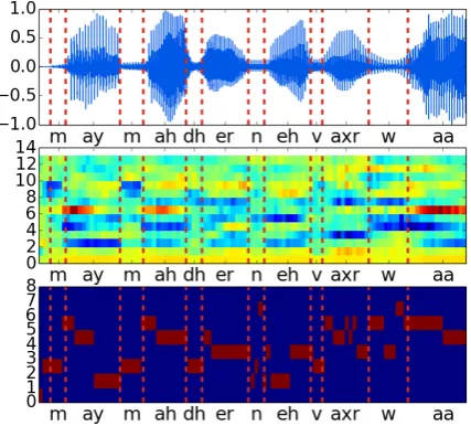
We used two kinds of speech features : 13 di-mensional MFCCs (Davis and Mermelstein,1980) (with 12 mel-cepstrum coefficients and 1 energy coefficient) and categorical one-hot vectors

de-rived from MFCCs inspired byR¨as¨anen(2014).

Figure 1: Visual representation of the various features on 100 frames from the TIMIT corpus. From top to bottom are the waveform, the 13-dimensional MFCCs and the 8-13-dimensional one hot encoded categorical features.

The latter are computed according to R¨as¨anen (2014) : K-means clustering1 _{is performed on a}

random subset of the MFCCs (10,000 frames were selected at random), with a target number of clus-ters of 8, then each MFCC is identified to the clos-est centroid. Each frame is then represented by a cluster numberc_{∈ {}1, . . . ,8_}, or alternatively by

the corresponding one-hot vector of dimension8.

These hyper-parameters were chosen according to R¨as¨anen(2014).

Figure1 allows for a visual comparison of the three signals (waveform, MFCC, categorical).

The entire dataset is split between a training and a testing subset. A randomly selected subset of the training part is used as validation data to prevent overfitting.

3.2 Training phase

A frame-by-frame prediction model is then learned on the training set. The three different models used are described below :

Pseudo-markov model When trying to pre-dict the frame xt given the previous frames xt₀−1:=xt−1, . . . , x0, a simplifying assumption is to model the transition probabilities with a Markov 1_{In particular, we use the K-means++ (Arthur and}

chain of higher orderK, i.e. p(xt|x0t−1) = p(xt | xt_t−₋1_K). Provided each frame is part of a finite

al-phabet, a finite (albeit exponential in K) number

of transition probabilities must be learned. However, as the order rises, the ratio between the size of the data and the number of transition probability being learned makes the exact calcula-tion more difficult and less relevant.

In order to circumvent this issue, we approxi-mate theK-order Markov chain with the mean of

1-order markov chain of the lag-transition proba-bilitiesp(xt|xt−i)for16i6K, so that

p(xt|xt0−1) =

1 K

K

X

i=1

p(xt|xt−i) (1)

withp(xt|xt−i) = f(_fx₍t_x,x_t−t−_i)i).

In practice, we choseK = 6, thus ensuring that

the markov model’s attention is of the same order of magnitude than the length of a phoneme.

Compared to R¨as¨anen (2014), this model only uses information from previous frames and as such is completely online.

Recurrent neural network on categorical fea-tures Alternatively to Markov chains, the tran-sition probability p(xt|xt0−1) can be modeled by a recurrent neural network (RNN). RNN can the-oretically model indefinite order temporal de-pendencies, hence their advantage over Markov chains for long sequence modeling.

Given a set of examples {(xt,(xt₀−1)) |

t _{∈ {}0, . . . , tmax}}, the networks parameters are

learned so that the error E(xt,RNN(xt0−1)) is minimized using back propagation through time (Werbos,1990) and stochastic gradient descent or a variant thereof (we have found RMSProp ( Tiele-man and Hinton,2012) to give the best results).

In our case, the network itself consists of two LSTM layers (Hochreiter and Schmidhuber,1997) stacked on one another followed by a linear layer and a softmax. The input and output units have both dimension 8, whereas all other layers have the same hidden dimension 40. Dropout ( Srivas-tava et al.,2014) with probability 0.2 was used af-ter each LSTM layer to prevent overfitting.

A pitfall of this method is the tendency of the network to predict the last frame it is fed. This is due to the fact that the sequences of categori-cal features extracted from speech contain a lot of constant sub-sequences length>2.

As a consequence, around 80% of the data fed to the network consists of sub-sequences where

xt = xt−1 . Despite the fact that phone bound-aries are somewhat correlated with changes of cat-egories (around 65% of the time), this leads the network to a local minimum where it only tries to predict the same characters.

To mitigate this effect, examples where xt = xt−1 were removed with probability 0.8, so that the number of transitions was slightly skewed to-wards category transitions. The model still passed over all frames during training but the error was back-propagated for only 46% of them. This change lead to substantial improvement.

Recurrent neural network on raw MFCCs

The recurrent neural network model can be adapted to raw speech features simply by changing the loss function from categorical cross-entropy to mean squared error, which is the direct translation from a categorical distribution to a Gaussian den-sity (2kx−yk2

2+dis the Kullback-Leibler diver-gence of two d-dimensional normal distributions

centered in x andy with the same scalar covari-ance matrix).

We used the same architecture than in the cat-egorical case, simply removing the softmax layer and decreasing the hidden dimension size to 20. In this case, no selection of the samples is needed since the sequences vary continuously.

3.3 Test phase

Each model is run on the test set and the prediction error is calculated at each time step according to the formula :

Emarkov(t) =−log

K X

i=1

p(xt|xt−i)

!

ERNN-cat(t) =−

d

X

i=1

1xt=ilog(RNN(x

t−1 0 ))

ERNN-MFCC(t) = 1 d

_xt−RNN(xt₀−1)2₂

(2)

In each case this corresponds, up to a scaling factor constant across the dataset, to the Kullback-Leibler divergence between the predicted and ac-tual probability distribution for xt in the feature

space.

Algorithm P R F R-val Periodic 57.5 91.0 70.5 46.9 Rasanen (2014) 68.4 70.6 69.5 73.7 Markov 70.7 77.3 73.9 76.4 RNN (Cat.) 68.7 77.1 72.7 74.6 RNN (Cont.) 70.3 72.4 71.3 75.3

Table 1: Final results (in%) evaluated with cropped tolerance windows

frames of each utterance. To be consistent, the first 7 frames (70 ms) of the error signal for each utter-ance were set to 0.

A peak detection procedure is then applied to the resulting error. As we are looking for sudden bursts in the prediction error, a local maximum is labeled as a potential boundary if and only if the difference between its value and the one of the pre-vious minimum is superior to a certain thresholdδ.

4 Experiments

4.1 Dataset

We evaluated our methods on the TIMIT dataset Fischer et al.(1986). The TIMIT dataset consists of 6300 utterances (∼5.4 hours) from 630 speak-ers spanning 8 dialects of the English language. The corpus was divided into a training and test set according to the standard split. The training set contains 4620 utterances (172,460 boundaries) and the test set 1680 (65,825 boundaries).

4.2 Evaluation

The performance evaluation of our system is based on precision (P), recall (R) andF-score, defined

as the harmonic mean of precision and recall. A drawback of this metric is that high recall, low precision results, such as the ones produces by hy-pothesizing a boundary every 5 ms (P : 58%, R : 91%) yield highF-score (70%).

Other metrics have been designed to tackle this issue. One such example is the R-value (R¨as¨anen et al.,2009) :

R-val= 1− q

(1₋R)2_+OS2_+|R+1_√−OS

2 |

2 (3)

Where OS = R_P −1 is the over-segmentation

measure. The R value represents how close the segmentation is from the ideal 0 OS, 1 R point and the P=1 line in the R, OS space. Further details can be found inR¨as¨anen et al.(2009).

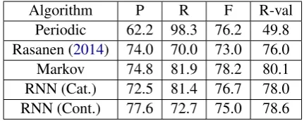
Algorithm P R F R-val

Periodic 62.2 98.3 76.2 49.8 Rasanen (2014) 74.0 70.0 73.0 76.0 Markov 74.8 81.9 78.2 80.1 RNN (Cat.) 72.5 81.4 76.7 78.0 RNN (Cont.) 77.6 72.7 75.0 78.6

Table 2: Final results (in%) evaluated with over-lapping tolerance windows. The scores reported forRasanen (2014)are the paper results.

Determining whether gold boundary is detected or not is a crucial part of the evaluation proce-dure. On our test set for instance, which contains 65,825 gold boundaries partitioned into 1,680 files, adding or removing one correctly detected boundary per utterance leads to a change of ± 2.5% in precision. This means that minor changes in the evaluation process (such as removing the trailing silence parts of each file, removing the opening and closing boundary) yield non-trivial variations in the end result.

A common condition for a gold boundary to be considered as ’correctly detected’ is to have a pro-posed boundary within a 20 ms distance on either side. Without any other specification, this means that a proposed boundary may be matched to sev-eral gold boundaries, provided these are within 40 ms from each other, leading to an increase of up to 4% F-score in some of our results (74%—78%). Unfortunately this point is seldom detailed in the literature.

We decided to use the procedure described in R¨as¨anen et al. (2009) to match gold boundaries and hypothesized boundaries : overlapping toler-ance windows are cropped in the middle of the two boundaries.

4.3 Results

The current state of the art in blind phoneme seg-mentation on the TIMIT corpus is provided by Hoang and Wang(2015). It evaluates to 78.16% F-score and 81.11 R-value on the training part of the dataset, using an evaluation method similar to our own.

our results with both evaluation methods (full win-dows and cropped winwin-dows) for the sake of con-sistency.

Another main difference with R¨as¨anen (2014) is that its results are given on the core test set of TIMIT, whereas our results are given on the full test set.

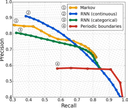
Figure 2: Precision/recall curves for our various models when varying the peak detection threshold

δ

Figure 2 provides an overview of the preci-sion/recall scores when varying the peak detec-tion threshold (and, in case of periodic boundaries, the period). This gives some insight about the ac-tual behavior of the various algorithms, especially in the high precision, low recall region where the RNN on actual MFCCs seems to outperform the methods based on discrete features.

We provide Figure3as a qualitative assessment of the error profiles of all three algorithms on one specific utterance. Notably, the error profile of the markov model contains distinct isolated peaks of similar height. As expected, the error curve is much more noisy in the case of the RNN on MFCCs, due to the greater variability in the fea-ture space.

5 Discussion

In terms of optimal F-score and R values, the sim-ple Markov model outperformed the previously published paper using short term sequential statis-tics (R¨as¨anen,2014), as well as the recurrent neu-ral networks. However, these optimal values may mask the differential behavior of these algorithms in different sections of the precision/recall curve.

In particular, it is interesting to notice that the neural network based model trained on the raw MFCCs gave very good results in the low recall, high precision domain. Indeed, the precision can reach 90% with a recall of 40%. Such a regime could be useful, for instance, if blind phoneme segmentation is used to help with word segmen-tation.

The reason of the higher precision of neural networks may be that it combines the sensitivity of this model to sequential statistical regularities of the signal, but also to the spectral variations, i.e. the error is also correlated to the spectral changes, meaning that some peaks are associated with a high error because the euclidean distance kxt+1−xtk2 itself is big. This is why the height

difference is much more significant in this case.

Figure 3: Comparison of error signals (gold boundaries are indicated in red)

Although we only reported the best results, we also tested our model on two other neural network architectures : a single vanilla RNN and a single LSTM cell. Both architecture did not yield signifi-cantly different results (∼1—2% F-score, mainly dropping precision). Similarly, different hidden dimension were tested. In the extreme cases (very low - 8 - or high - 128 - dimension), the output signal proved too noisy to be of any significance, yielding results comparable to naive periodic seg-mentation.

6 Conclusions

We have presented a lightweight blind phoneme segmentation method predicting boundaries at peaks of the prediction loss of transition probabil-ities models. The different models we tested pro-duced satisfying results while remaining computa-tionally tractable, requiring only one pass over the data at test time.

Our recurrent neural network trained on speech features in particular hints at a way of combining both the statistical and spectral information into a single model.

On a machine learning point of view, we high-lighted the use that can be made of side channel information (in this case the test error) in order to extract structure from raw data in an unsupervised setting.

Future work may involve exploring different RNN models, assessing the stability of these meth-ods on simpler features such as raw spectrograms or waveforms, or exploring the representation of each frame in the hidden layers of the networks.

7 Acknowledgements

The authors would like to thank the anonymous re-viewers for their insightful and constructive com-ments which helped shape the final version of this paper.

This project is supported by the Euro-pean Research Council (ERC-2011-AdG-295810 BOOTPHON), the Agence Nationale pour la Recherche (LABX-0087 IEC, ANR-10-IDEX-0001-02 PSL*), the Fondation de France, the Ecole de Neurosciences de Paris, the Region Ile de France (DIM cerveau et pens´ee), and an AWS in Education Research Grant award.

References

George Almpanidis and Constantine Kotropoulos. 2008. Phonemic segmentation using the generalised gamma distribution and small sample bayesian information criterion. Speech Communication

50(1):38–55.

David Arthur and Sergei Vassilvitskii. 2007. k-means++: The advantages of careful seeding. In

Proceedings of the eighteenth annual ACM-SIAM symposium on Discrete algorithms. Society for In-dustrial and Applied Mathematics, pages 1027– 1035.

Morten H Christiansen, Joseph Allen, and Mark S Sei-denberg. 1998. Learning to segment speech using

multiple cues: A connectionist model. Language and cognitive processes13(2-3):221–268.

Steven Davis and Paul Mermelstein. 1980. Compari-son of parametric representations for monosyllabic word recognition in continuously spoken sentences.

IEEE transactions on acoustics, speech, and signal processing28(4):357–366.

Sorin Dusan and Lawrence R Rabiner. 2006. On the relation between maximum spectral transition posi-tions and phone boundaries. InProceedings of In-terspeech. Citeseer.

Jeffrey L Elman. 1990. Finding structure in time. Cog-nitive Science14(2):179–211.

Anna Esposito and Guido Aversano. 2005. Text inde-pendent methods for speech segmentation. In Non-linear Speech Modeling and Applications, Springer, pages 261–290.

Yago Pereiro Estevan, Vincent Wan, and Odette Scharenborg. 2007. Finding maximum margin seg-ments in speech. In2007 IEEE International Con-ference on Acoustics, Speech and Signal Processing-ICASSP’07. IEEE, volume 4, pages IV–937.

William M. Fischer, George R. Doddington, and Kath-leen M Goudie-Marshall. 1986. The darpa speech recognition research database: Specifications and status. In Proceedings of DARPA Workshop on Speech Recognition. pages 93–99.

James R Glass. 2003. A probabilistic framework for segment-based speech recognition. Computer Speech & Language17(2):137–152.

Dac-Thang Hoang and Hsiao-Chuan Wang. 2015. Blind phone segmentation based on spectral change detection using legendre polynomial approximation.

The Journal of the Acoustical Society of America

137(2):797–805.

Sepp Hochreiter and J¨urgen Schmidhuber. 1997. Long short-term memory. Neural computation

9(8):1735–1780.

Herman Kamper, Aren Jansen, and Sharon Goldwater. 2015. Fully unsupervised small-vocabulary speech recognition using a segmental bayesian model. In

Proceedings of Interspeech.

Vahid Khanagha, Khalid Daoudi, Oriol Pont, and Hus-sein Yahia. 2014. Phonetic segmentation of speech signal using local singularity analysis. Digital Sig-nal Processing35:86–94.

Yu Qiao, Naoya Shimomura, and Nobuaki Minematsu. 2008. Unsupervised optimal phoneme segmenta-tion: Objectives, algorithm and comparisons. In

Okko R¨as¨anen. 2014. Basic cuts revisited: Temporal segmentation of speech into phone-like units with statistical learning at a pre-linguistic level. In Pro-ceedings of the 36th Annual Conference of the Cog-nitive Science Society. Quebec, Canada.

Okko Rasanen, Toomas Altosaar, and Unto Laine. 2011. Blind segmentation of speech using non-linear filtering methods. INTECH Open Access Publisher.

Okko R¨as¨anen, Unto Kalervo Laine, and Toomas Al-tosaar. 2009. An improved speech segmentation quality measure: the r-value. InProceedings of In-terspeech.

Man-hung Siu, Herbert Gish, Arthur Chan, William Belfield, and Steve Lowe. 2013. Unsupervized training of an HMM-based self-organizing recog-nizer with applications to topic classification and keyword discovery. Computer Speech & Language

preprint.

Nitish Srivastava, Geoffrey E Hinton, Alex Krizhevsky, Ilya Sutskever, and Ruslan Salakhutdinov. 2014. Dropout: a simple way to prevent neural networks from overfitting. Journal of Machine Learning Re-search15(1):1929–1958.

Tijmen Tieleman and Geoffrey Hinton. 2012. Lecture 6.5-rmsprop: Divide the gradient by a running av-erage of its recent magnitude. COURSERA: Neural Networks for Machine Learning4(2).

Paul J Werbos. 1990. Backpropagation through time: what it does and how to do it. Proceedings of the IEEE78(10):1550–1560.

Robert Wilber. 1988. The concave least-weight sub-sequence problem revisited. Journal of Algorithms