Munich Personal RePEc Archive
Effect of Aging on Housing Prices: A
Perspective from an Overlapping
Generation Model
Sun, Tianyu and Chand, Satish and Sharpe, Keiran
UNSW Canberra
10 February 2018
Online at
https://mpra.ub.uni-muenchen.de/94419/
1
Effect of Aging on Housing Prices: A Perspective from an
Overlapping Generation Model
Tianyu Sun
*, Satish Chand and Keiran Sharpe
ABSTRACT
This paper investigates the effect of aging on housing prices. It provides a theoretical explanation to address the on-going debate about the impact of aging on house prices. The analysis demonstrates that aging has divergent effects on housing prices, depending on the net
effects of a fall in fertility vis-à-vis a rise in longevity on demand for housing. In addition, the results suggest that aging can produce a turning point in the price dynamics. To the left of the peak, aging boosts prices while to the right, it has the opposite effect. Furthermore, inequality of household utility is enlarged during the aging processes.
JEL classification: E21, E31, J11, R21, R31
Keywords: Aging Population; OLG Model; House Prices; Land Prices; Turning Point
*
Corresponding author.
Email addresses: [email protected] (T. Sun), [email protected] (S. Chand), [email protected] (K. Sharpe).
2 1. Introduction
Will an aging population affect housing prices? The extant literature provides divergent answers to this question. The first argues that an aging population will have a significant effect on housing prices (Mankiw and Weil 1989, 1991, Bergantino 1998, Takáts 2012), and the second opined that aging would have little or mixed impact (Engelhardt and Poterba 1991, Hendershott 1991, Poterba 2001, Eichholtz and Lindenthal 2014, Hiller and Lerbs 2016). The debate on the impact of aging on housing prices is largely drawn from empirical studies, and remains alive (Poterba 2014). This paper contributes to the extant literature by investigating the effects of aging within the context of an overlapping generations model (OLG) to explain the mixed results from empirical studies estimating the effects of aging on housing prices.
The results show that an aging population can result from a fall in fertility and/or an increase
in longevity: housing prices increase only when the net effect of the above is positive. More specifically, a fertility rate lower than the replacement level will depress housing prices while
an increase in longevity has the opposite effect. The above explains some of the divergent effects of an aging population on housing prices in different contexts. From this perspective, the seemingly contradictory views from previous empirical research can be reconciled.
3
Our paper fits into the emerging literature on housing prices using theoretical models.1 While this literature has focused on various factors underscoring the demand for housing, it has not addressed the impact of aging that we focus on here. In addition, our paper also contributes to the literature on the consequences of aging on the accumulation of assets and savings.2 The
bulk of theoretical work in this area has ignored housing as an asset, a major deficiency given
that housing is the largest component of households’ wealth. We address this void in the literature.
We first model the long-term effect of an aging population on housing prices, and then simulate the dynamics of housing prices due to demographic changes. Although our work aims to reach general conclusions about the effects of aging, the results are based on simulations that in turn are sensitive to the parameters of the model. Our parameters are calibrated for China for two compelling reasons: (i) housing assets constitute more than 70 percent of Chinese
households’ wealth (Xie and Jin 2015); and, (ii) China is undergoing rapid aging of its population (Lutz, Sanderson, and Scherbov 2008). Thus, choosing the parameters for China provides us with a typical example without losing the generality of the conclusions.
Our results show that demographic change has a bigger impact on land prices than that for construction, a fact revealed only when the two are looked at separately. This result is consistent with the empirical findings of Davis and Heathcote (2007). Specifically, our simulations show that a decline in the fertility rate of 10 percent from the replacement level for one generation (i.e. 30 years in our model) leads to a fall in the price of construction by 1 percent whereas the price of land falls by 10 percent. In contrast, when longevity increases by 6 percent then the corresponding house and land prices increase by 1 percent and 7 percent,
respectively.
We next investigate the effects of a simultaneous change in fertility and longevity on
households’ utility. Anticipating the results, workers would have greater utility because of higher house and land ownership per capita; however, the utility of the retirees is worse. Assuming perfect foresight in the model, the consequential housing prices would increase immediately before the demographic changes and decline as the effects of the fall in fertility take over.
1
See, for example, Iacoviello (2005); Iacoviello and Neri (2010); Liu, Wang, and Zha (2013); Justiniano, Primiceri, and Tambalotti (2015); Ng (2015); Chen and Wen (2017).
2
4
The remainder of this paper is organized as follows. Section 2 describes the OLG model, Section 3 presents the assumptions and the calibration of parameters, while section 4 shows the solution method. Section 5 presents the long-term effects of aging on housing prices, and section 6 investigates household utility and the housing price dynamics. Section 7 concludes.
2. The Model
2.1. Demography
The model’s time structure is the same as the classical model of Diamond (1965). The economy consists of two overlapping generations, namely, workers and retirees, who are alive in both periods. For each generation, we assume that the households are identical.3
The population of workers is affected only by the rate of fertility. The fertility rate at time t,
denoted by 𝑛𝑡, is given as equation (1), where 𝑁𝑡,1 and 𝑁𝑡−1,1 represent the population of workers at time t and its previous period, respectively. Note that in this stylized model, the
fertility rate is equal to the rate of growth of workers.
𝑛𝑡= 𝑁𝑁𝑡,1
𝑡−1,1 (1)
The population of retirees, in contrast, is influenced by both the fertility rate and longevity. Following Blackburn and Cipriani (2002) and Cipriani (2013), longevity is defined by the share of households that survive to retirement stage. Specifically, households are alive as workers with certainty, but a fraction die at the beginning of their retirement, while the rest live for the remaining period of retirement. This survival function is given as equation (2), where 𝑁𝑡−1,1 and 𝑁𝑡,2 represent the number of workers in period 𝑡 − 1 and the retirees in period t respectively.
𝜋𝑡 =𝑁𝑁𝑡,2
𝑡−1,1 (2)
Based on (1) and (2), the population dynamics of retirees is given as:
𝑁𝑡,2
𝑁𝑡−1,2=
𝑛𝑡−1𝜋𝑡
𝜋𝑡−1 (3)
3
5
2.2. Households
Utility
The households’ utility is characterized by (4) as follows:
𝑈𝑡= 𝑈( 𝑈𝑡,1, 𝑈𝑡+1,2) = 𝑈𝑡,1+ 𝜋𝑡+1 𝛽 𝐸(𝑈𝑡+1,2) (4)
Following Diamond (1965), the expected life span utility of a household (𝑈𝑡) is time separable and is determined by the sum of utility when working, 𝑈𝑡,1 and that when retired,
𝑈𝑡+1,2. Two discount factors are 1) the time preference 𝛽 (0 < 𝛽 < 1) and 2) the survival rate
𝜋. The form of equation (4) is consistent with the practice that survival rates are involved.4 The utility during work (𝑈𝑡,1) is given as:
𝑈𝑡,1 = ln(𝑐𝑡,1) + 𝑗ℎln(ℎ𝑡,1) + 𝑗𝑙ln(𝑙𝑡,1) −1 + 𝜂 (𝑛𝜏 𝑐,𝑡1+𝜉+ 𝑛ℎ,𝑡1+𝜉) 1+𝜂
1+𝜉 (5)
Following Iacoviello and Neri (2010) and Liu, Wang, and Zha (2013), the terms providing positive utility in (5) are per capita consumption of goods, 𝑐𝑡,1, structure of houses, ℎ𝑡,1, and land, 𝑙𝑡,1. Variables 𝑛𝑐,𝑡 and 𝑛ℎ,𝑡 represent hours worked in non-housing and housing sectors respectively. The negative term on the far right of (5) represents the disutility of work.
First, we explain why both the building and land are in the utility function. Housing provides utility and consists of the construction and land. However, the literature includes either the structure or the land in the utility function. We include both, and each contributes to utility separately. We assume that land provides utility above and beyond the building that sits on it. For example, the houses that occupy bigger land (e.g. villas) provide additional utility compared to apartments of identical residential space. This may be rationalised as green space
providing utility of its own. This preference is supported by scholarship within psychology.5 Back to the equation (5), the parameters 𝑗ℎ and 𝑗𝑙 represent the preference for house and land respectively, and the parameter 𝜏 denotes the disutility of work. The parameter 𝜂 > 0 ensures that the utility function is concave with respect to labour supply. In addition, the parameter 𝜉 >
0 indicates the labour mobility between the two production sectors is imperfect (Horvath 2000, Iacoviello and Neri 2010).
The utility function for the retirees, who do not participate in the labour market, is analogous to (5); that is,
𝑈𝑡+1,2 = ln(𝑐𝑡+1,2) + 𝑗ℎln(ℎ𝑡+1,2) + 𝑗𝑙ln(𝑙𝑡+1,2) (6)
4
See, for example, Blackburn and Cipriani (2002), Cipriani (2013) and Muto, Oda, and Sudo (2016) 5
6
, where the consumption, house and land per capita of this generation are denoted by 𝑐𝑡+1,2,
ℎ𝑡+1,2 and 𝑙𝑡+1,2 respectively.
Budget Constraint
The budget constraint for individual worker is as follows:
𝑐𝑡,1+ 𝑞𝑡ℎ𝑡,1+ 𝑝𝑙,𝑡𝑙𝑡,1= (1 − 𝑇)(𝑤𝑐,𝑡𝑛𝑐,𝑡+ 𝑤ℎ,𝑡𝑛ℎ,𝑡+ 𝑑𝑡) (7)
, where the right side is the income of the workers and the left side is the expenditures. The income can be divided into wage, 𝑤𝑐,𝑡𝑛𝑐,𝑡+ 𝑤ℎ,𝑡𝑛ℎ,𝑡, and dividend, 𝑑𝑡, income. Workers pay tax of T, and thus the fraction (1 − 𝑇) is the share of the income kept by the workers while the
remainder accrues to the retirees. One could rationalize the specification of ‘T’ in (7) as a pay -as-you-go pension system where the current generation of workers are taxed to fund consumption of the retirees.
The expenditure is 𝑐𝑡,1+ 𝑞𝑡ℎ𝑡,1+ 𝑝𝑙,𝑡𝑙𝑡,1, where 𝑞𝑡 and 𝑝𝑙,𝑡 denote the prices of structure and land respectively. The households do not have deposits because it equals the loans to the firms. However, the firms are assumed to be owned by all the households collectively. Thus, for any individual, one cannot retrieve the capital of firms for consumption. Instead, households have the right to claim for the profits of the firms, i.e. the dividend 𝑑𝑡 in equation (7). Further illustration can be found in the section of firms.
The budget constraint for individual retiree is as follows:
𝑐1+𝑡,2+ 𝑞1+𝑡ℎ1+𝑡,2+ 𝑝𝑙,1+𝑡𝑙1+𝑡,2 =
𝑇(𝑑1+𝑡+ 𝑛𝑐,1+𝑡𝑤𝑐,1+𝑡+ 𝑛ℎ,1+𝑡𝑤ℎ,1+𝑡)𝜋𝑛1+𝑡
1+𝑡+ (8)
𝑞1+𝑡(1 − 𝛿ℎ) (𝜋ℎ𝑡,1 1+𝑡+
𝜋𝑡ℎ𝑡,2
𝜋1+𝑡𝑛𝑡) + 𝑝𝑙,1+𝑡(
𝑙ℎ,𝑡,1
𝜋1+𝑡+
𝜋𝑡𝑙𝑡,2
𝜋1+𝑡𝑛𝑡)
The right part of (8) is the income of retirees, while the left part is expenditures. The revenues accruing to the retirees have some differences with that of workers because the revenues consist of three parts: 1) the pension payments; 2) the wealth accumulated previously; and 3) inheritances. The aggregate values of these revenues are listed in Table 1, and the per capita values can be derived according to the equations (1), (2) and (3) by dividing the totals by the population of retirees, 𝑁1+𝑡,2.
7
Table 1—Aggregate market values of retirees’ income
Pensions 𝑻(𝒅𝟏+𝒕𝑵𝟏+𝒕,𝟏+ 𝒏𝒄,𝟏+𝒕𝒘𝒄,𝟏+𝒕𝑵𝟏+𝒕,𝟏+ 𝒏𝒉,𝟏+𝒕𝒘𝒉,𝟏+𝒕𝑵𝟏+𝒕,𝟏) Wealth 𝜋𝑡+1(𝑞𝑡+1(1 − 𝛿ℎ)ℎ𝑡,1𝑁𝑡,1+ 𝑝𝑙,𝑡+1𝑙𝑡,1𝑁𝑡,1)
Inheritances 𝑞𝑡+1(1 − 𝛿ℎ)ℎ𝑡,2𝑁𝑡,2+ 𝑝𝑙,𝑡+1𝑙𝑡,2𝑁𝑡,2+
(1 − 𝜋𝑡+1)𝑞𝑡+1(1 − 𝛿ℎ)ℎ𝑡,1𝑁𝑡,1+ (1 − 𝜋𝑡+1)𝑝𝑙,𝑡+1𝑙𝑡,1𝑁𝑡,1
Note: 𝛿ℎ represents depreciation rate of houses.
In particular, the inheritance is in the form of houses (and land) and assumed to be so for three reasons. First, housing is needed by every individual, including the retired. Second, houses cannot be fully consumed by their owners, even at the time of their death. Third, houses are bequeathed to the next generation. For example, during the study of the bequest decision of Australians, Ding (2012) stated that housing assets constitute the bulk of bequests.
In our model, inheritance comes from two sources: 1) the previous generation of retirees,
whose population is 𝑁𝑡,2; and 2) the workers who do not survive to retirement, whose population is (1 − 𝜋𝑡+1)𝑁𝑡,1. The market values of these two parts are 𝑞𝑡+1(1 − 𝛿ℎ)ℎ𝑡,2𝑁𝑡,2+
𝑝𝑙,𝑡+1𝑙𝑡,2𝑁𝑡,2 and (1 − 𝜋𝑡+1)𝑞𝑡+1(1 − 𝛿ℎ)ℎ𝑡,1𝑁𝑡,1+ (1 − 𝜋𝑡+1)𝑝𝑙,𝑡+1𝑙𝑡,1𝑁𝑡,1 respectively,
where 𝛿ℎ represents that rate of depreciation of houses. Meanwhile, the market value of house and land purchased during their working period is 𝜋𝑡+1(𝑞𝑡+1(1 − 𝛿ℎ)ℎ𝑡,1𝑁𝑡,1+ 𝑝𝑙,𝑡+1𝑙𝑡,1𝑁𝑡,1). Thus, the total market value of the housing wealth is obtained by adding these parts together
and is represented as 𝑞𝑡+1(1 − 𝛿ℎ)ℎ𝑡,1𝑁𝑡,1+ 𝑝𝑙,𝑡+1𝑙𝑡,1𝑁𝑡,1.
2.3. Firms
The other agent in the economy is the firms. We adapt the model in Liu, Wang, and Zha
(2013) where firms are assumed to exist forever, and they have three important functions. The first is that they produce goods for consumption and housing, and this function will be illustrated in the section on technology. Furthermore, the firms invest in and maintain plant and equipment. Finally, firms maximize profits with the proceeds paid to households in the form of dividends.
Profit maximization
Following Liu, Wang, and Zha (2013), firms maximize long-run profits, denoted as follows:
𝑀𝑎𝑥 ∑ 𝛽𝑒𝑡ln(𝐷𝑡) 𝑡
8
, where 𝐷𝑡 = 𝑑𝑡𝑁𝑡,1 represents the total profits of the firms in period t. In addition, the parameter 𝛽𝑒 represents the time preference of firms. Additionally, the time preference of firms is less than that of the households, i.e. 𝛽𝑒 < 𝛽, lending the incentive to invest (Iacoviello 2005, Liu, Wang, and Zha 2013, Iacoviello 2015). By using the log-function in (9), we assume that the firm prefers stable profit flow. This assumption follows from risk-aversion by households who own these firms (Sandmo 1971, Leland 1972, Oh, Rhodes, and Strong 2016).
A major modification from Liu, Wang, and Zha (2013) is that, in our model, the firms are assumed to be owned by all the households instead of a certain fraction of them. This modification allows us to focus on the households’ heterogeneity of age structures without the complication of income distribution. Without this modification, as shown in Liu, Wang, and Zha (2013), the entrepreneurs would be introduced as a distinct class from the employees.
Here, we further provide microeconomic explanations about the assumed ownership of the firms above. To begin with, the economy consists of many firms. When viewing the firms together, it works as the firms in our model. In addition, every firm is owned by some households, while every household is one of the owners of some firms because we have no distinction between entrepreneurs and employees. Lastly, the households have full insurance on their wage and profits, thus their income is subject to the performance of the aggregate economy.
One of the consequences of the setting above is that households do not have deposits. Because the deposit is held as capital of firms, the households as owners of firms do not need separate deposit accounts. According to (16), the capital can be adjusted and distributed to households in the form of profit. From this point of view, the personal deposits are not disappeared but pooled in the total capitals. A possible drawback is that this saving is the same for all the households; nevertheless, modelling wealth distribution aside from the housing asset is beyond the scope of this paper.
Furthermore, we will explain why we have 𝛽𝑒 < 𝛽 based on the setting above. Although each firm is owned by a panel of households, the time that the panel can own this firm will be no more than the longevity of households (because only living people can be on the panel). Thus, the firm owners, although they are households, will be more impatient about the future of firms than their own lives. This explanation is consistent with the reality that the survival rates of firms are less than that of the households.
9
An often cited omission from previous research on the effect of aging population on housing prices is the supply side of the market (Swan 1995). We follow Iacoviello and Neri (2010) and treat the supply of housing as a separable production sector from the non-housing productions.
Non-housing production sector: The non-housing sector uses Cobb-Douglas technology of the form:
𝑌𝑡 = 𝐴𝑐,𝑡𝐾𝑐,𝑡−1𝜇𝑐 𝑁𝑐,𝑡1−𝜇𝑐 (10)
The non-housing production is denoted by 𝑌𝑡 = 𝑦𝑡𝑁𝑡,1, and there are three types of variables involved in the production process: the aggregate capital of non-housing production sector,
𝐾𝑐,𝑡−1 = 𝑘𝑐,𝑡−1𝑁𝑡−1,1; the labour employed, 𝑁𝑐,𝑡 = 𝑛𝑐,𝑡𝑁𝑡,1; and the Total Factor Productivity
(TFP) in the non-housing production sector, 𝐴𝑐,𝑡.
Housing production sector: Similar to that of the non-housing production sector, housing production takes the form:
IH𝑡 = 𝐴ℎ,𝑡𝐾ℎ,𝑡−1𝜇ℎ 𝐿𝜇𝑒,𝑡−1𝑙 𝑁ℎ,𝑡1−𝜇ℎ−𝜇𝑙 (11)
The houses built by the housing production sector is denoted by IH𝑡 = 𝑖ℎ𝑡𝑁𝑡,1. The construction of houses needs capital 𝐾ℎ,𝑡−1 = 𝑘ℎ,𝑡−1𝑁𝑡−1,1, land (which is owned by the firms)
𝐿𝑒,𝑡−1= 𝑙𝑒,𝑡−1𝑁𝑡−1,1, and labour 𝑁ℎ,𝑡 = 𝑛ℎ,𝑡𝑁𝑡,1 while TFP growth is denoted by 𝐴ℎ,𝑡.
Following the work of Iacoviello and Neri (2010), we assume the land is indispensable for the production of housing.
Capital Accumulation
We denote the investments in non-housing and housing sectors in period t as IK𝑐,𝑡 = 𝑖𝑘𝑐,𝑡𝑁𝑡,1 and IKℎ,𝑡 = 𝑖𝑘ℎ,𝑡𝑁𝑡,1 respectively. Following Liu, Wang, and Zha (2013), the capital accumulation processes for the non-housing and housing sectors are assumed to have the following specifications:
𝐾𝑐,𝑡 = (1 − 𝛿kc)𝐾𝑐,𝑡−1+ IK𝑐,𝑡− Φ𝑐,𝑡 (12)
𝐾ℎ,𝑡 = (1 − 𝛿kh)𝐾ℎ,𝑡−1+ IKℎ,𝑡− Φℎ,𝑡 (13)
, where parameters 𝛿kc and 𝛿kh represent the depreciation rates of capital in the non-housing and housing sectors respectively.
10
because it is the sum of the cost that happens within this period. We use Φ𝑐,𝑡 and Φℎ,𝑡 to denote the accumulated adjustment cost of non-housing and housing sectors in period t. Following Iacoviello and Neri (2010) and Liu, Wang, and Zha (2013), they have the following
specifications:
Φ𝑐,𝑡 = Φ𝑐(𝐾𝑐,𝑡, 𝐾𝑐,𝑡−1) =𝜙2 (𝑘𝑐 𝐾𝐾𝑐,𝑡
𝑐,𝑡−1− exp (𝑔𝐾𝐶,𝑡)) 2
𝐾𝑐,𝑡−1 (14)
Φℎ,𝑡= Φℎ(𝐾ℎ,𝑡, 𝐾ℎ,𝑡−1) =𝜙2 (𝑘ℎ 𝐾𝐾ℎ,𝑡
ℎ,𝑡−1− exp (𝑔𝐾𝐻,𝑡)) 2
𝐾ℎ,𝑡−1 (15)
, where 𝜙𝑘𝑐 and 𝜙𝑘ℎ are the parameters that represent the specific frictions in adjusting the capital stocks in non-housing and housing sectors respectively. In addition, variables 𝑔𝐾𝐶,𝑡 and
𝑔𝐾𝐻,𝑡 denote the trend capital growth rates on which the corresponding adjustment cost would
be zero. The trend growth rate will be illustrated in the section of solution method.
Budget Constraint
The aggregate budget constraint of the firms is as follows:
𝐷𝑡+𝐴𝐾𝑐,𝑡
𝑘,𝑡+ 𝐾ℎ,𝑡+ 𝑤𝑐,𝑡𝑁𝑐,𝑡+ 𝑤ℎ,𝑡𝑁ℎ,𝑡+ 𝑝𝑙,𝑡𝐿𝑒,𝑡+ Φ𝑐,𝑡
𝐴𝑘,𝑡+ Φℎ,𝑡
= 𝑌𝑡+ 𝑞𝑡 IH𝑡+1−𝛿𝐴𝑘,𝑡kc𝐾𝑐,𝑡−1+ (1 − 𝛿kh)𝐾ℎ,𝑡−1+ 𝑝𝑙,𝑡𝐿𝑒,𝑡−1 (16)
The right side of the (16) is the resources available to the firms while the left side is the
payments for the above. Firms have revenues from: 1) selling non-housing and housing productions; 2) the balance of capital after depreciation, and 3) the market value of land owned by the firm. For the capital in the non-housing sector, as in Iacoviello and Neri (2010), the investment specific technology shock is introduced to the model and denoted by 𝐴𝑘,𝑡.
The distribution of this wealth can be divided into four parts. Firstly, firms pay profits to households, as denoted by 𝐷𝑡 in (16). Secondly, the capital stocks for next period are decided by the firms, which are denoted as 𝐾𝑐,𝑡 and 𝐾ℎ,𝑡. Along with this process, the capital adjustment costs are involved (Φ𝑐,𝑡 and Φℎ,𝑡). Thirdly, wages are paid to the workers. Lastly, the firms will decide on the amount of land owned in this period.
2.4. Equilibrium
11
factors are equal to their marginal contributions. The equilibrium conditions of the first three markets are:
𝑌𝑡 = 𝐶𝑡+IK𝐴𝑐,𝑡
𝑘,𝑡 + IKℎ,𝑡+ Φ𝑡 (17)
𝐻𝑡 = IH𝑡+ (1 − 𝛿ℎ)𝐻𝑡−1 (18)
𝐿𝑡 = 𝐿ℎ,𝑡+ 𝐿𝑒,𝑡 (19)
, where 𝐶𝑡= 𝑐𝑡,1𝑁𝑡,1+ 𝑐𝑡,2𝑁𝑡,2, 𝐻𝑡 = ℎ𝑡,1𝑁𝑡,1+ ℎ𝑡,2𝑁𝑡,2, 𝐿ℎ,𝑡 = 𝑙ℎ,𝑡,1𝑁𝑡,1+ 𝑙ℎ,𝑡,2𝑁𝑡,2, 𝑌𝑡 =
𝑦𝑡𝑁𝑡,1, 𝐻𝑡= ℎ𝑡𝑁𝑡,1, 𝐿𝑡= 𝑙𝑡𝑁𝑡,1.
For the labour market, its equilibrium means the labour supply of households would be equal to the labour demand of firms. This equilibrium amount of working hours has been denoted by
𝑁𝑐,𝑡 and 𝑁ℎ,𝑡 in the previous discussion (or per worker, 𝑛𝑐,𝑡 and 𝑛ℎ,𝑡).
3. Assumptions and Calibration
3.1. Demographic Assumptions
In this research, we study both the effects of a decline in the fertility rate and an increase in longevity on housing prices. The levels of the decline and increase are arbitrarily chosen; however, the analysis on them will be sufficient to show the general housing price dynamics
before, during and after the aging population process.
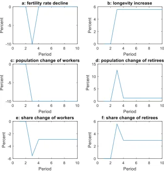
Specifically, at the period 1 and 2, the fertility rate is set at the replacement level. Using variable 𝛾𝑁,𝑡 to represent the rate of growth of the worker population, then 𝛾𝑁,1= 𝛾𝑁,2 = 0. The first shock is a fall in the fertility rate of 10 percent in period 3 (Figure 1a), and this fall is foreseen by the agents of the economy beforehand. Correspondingly, we have 𝛾𝑁,3 = −0.1. In period 4, the fertility rate is returned to the replacement level as its original state and kept stable from then on (Figure 1a). For worker population, it means that 𝛾𝑁,𝑡 = 0, 𝑡 ≥ 4.
The second shock is an increase in the survival rates 𝜋𝑡. Correspondingly, the longevity increases. In period 1 and 2, we assume that 𝜋1 = 𝜋2 = 0.8. In period 3, the survival rate increases to 0.9 and remains constant thereafter, i.e. 𝜋𝑡 = 0.9, 𝑡 ≥ 3. Again, the longevity changes are known by the agents of the economy beforehand. With the assumed increase in survival rate, total longevity increases by 5.56 percent6 (see Figure 1b).
By assuming both the changes above, the overall demographic changes regarding with the aging population are shown in Figure 1. The population of workers has declined (Figure 1c),
6
12
[image:13.595.133.470.158.509.2]while the population of retirees spikes at period 3, before stabilising after period 4 (Figure 1d). During this process, the proportion of retirees rises from period 2 to 3. After that, it declines and then stays the same (Figure 1f).
Figure 1. Overall Effect: Demography Changes
3.2. Parameter Calibration
To present the result numerically, we need assign values for the parameters. In this paper, we seek for feasible parameter values that fit the case of China because it will be a typical example when examining the effects of ageing on housing prices. For the parameters that has not been found under the context of China, we use the ones of America as a substitution.
13
The time preference of households 𝛽is calibrated to match China’s average real interest rates during 1980–20157. According to World Development Indicators database8, this rate, rounded to two decimal places, is 2 percent, which indicates the annual discount factor of
[image:14.595.87.508.237.540.2]0.98, and for a period of thirty years, we set 𝛽 = 0.55. Besides, following Iacoviello and Neri (2010) and Ng (2015), the annual discount rate of firms is set as 0.958 (=0.98/1.0232), lower than that of the households. In thirty years, the corresponding discount rate of firms 𝛽𝑒 is 0.275.
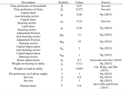
Table 2—Parameter Calibration of the Model
Description Symbols Values Sources Time preference of households 𝛽 0.55 See text Time preference of firms 𝛽𝑒 0.275 See text
Capital share
(non-housing sector) 𝜇𝑐 0.46 Ng (2015) Capital share
(housing sector) 𝜇ℎ 0.24 See text Land share
(housing sector) 𝜇𝑙 0.10 Ng (2015) Adjustment Friction
(non-housing sector) 𝜙kc 11 Ng (2015) Adjustment Friction
(housing sector) 𝜙kh 10 Ng (2015) Capital depreciation
(non-housing sector) 𝛿kc 1 Ng (2015) Capital depreciation
(housing sector) 𝛿kh 1 Ng (2015) House depreciation 𝛿ℎ 0.7 Iacoviello and Neri (2010) Weight on housing in utility 𝑗ℎ 0.12 Ng (2015)
Weight on land in utility 𝑗𝑙 0.045 Liu, Wang, and Zha (2013) Dis-preference on Labour supply 𝜏 1 Ng (2015)
See text 𝜂 0.5 Ng (2015)
See text 𝜉 1 Ng (2015)
Pension share 𝑇 0.4 Iacoviello and Pavan (2013)
There are three depreciation rates in our model. For the two types of capital in the production sectors, their annual depreciation rates are about 10 percent (Iacoviello and Neri 2010, Ng 2015). In thirty years, this depreciation rate implies that the initial capital stock is fully
depreciated. Thus, the corresponding parameters 𝛿kc and 𝛿kh are calibrated as 1. The depreciation rate of houses is calibrated according to Iacoviello and Neri (2010) as 4 percent annually9, indicating 70 percent depreciation of the stock in 30 years.
7
Follow Blackburn and Cipriani (2002) and Muto, Oda, and Sudo (2016), the survival rates in the utility function do not influence the calibration methods of the parameter of time preference.
8
World Development Indicator of the World Bank: Real interest rate.
Website: http://data.worldbank.org/indicator/FR.INR.RINR. Date of Access: 21/Apr/2017 9
14
The parameters denoting income shares and weight of utility are calibrated according to Ng (2015) and Liu, Wang, and Zha (2013). Their values are listed in Table 2: the capital share in
housing sector (𝜇ℎ) is set at 0.2410. The capital adjustment cost in the non-housing and housing sector is calibrated according to Ng (2015), and the values are reported in Table 2. Among all the parameters, the value of pension share 𝑇 of China has not been found in similar studies.
Here, we use the case of America as an alternative, and the value is calibrated according to the work of Iacoviello and Pavan (2013).
4. Solution method
Regarding the demographic changes, there are two exogenous variables in our model, i.e. the worker population growth rate, 𝛾𝑁,𝑡, and the survival rate, 𝜋𝑡. When the values of these exogenous variables change, their effects can be captured by the simulation11.
However, when the worker population growth rate is negative as in our assumptions, the worker population declines permanently (see figure 1c). Because the worker population is not a variable in the model of per capita variables, we cannot use the simulations to detect the effect of this permanent change.
To see this, note that the worker population growth rates are zero in both the original and end
state. Thus, we will get the same value of the per worker land area 𝑙 for both the states from the simulation (if consider the changes in 𝛾𝑁,𝑡 only). Nevertheless, when the total land area is a constant, we know that the per worker land area 𝑙 will increase by 10 percent if the worker population declines by 10 percent. The values of other variables may also be affected, but the influence cannot be shown by the simulation. In this study, the influences are denoted by the trends of variables because they are determining the levels of variables.
Besides the worker population, the changes in TFPs (𝐴𝑐,𝑡, 𝐴ℎ,𝑡, 𝐴𝑘,𝑡) and land area 𝐿𝑡 will also affect the levels of variables, and these effects are captured by the trend. Incorporating these factors are for general concerns to reveal their effects, and they will be assumed to be constants afterward. Correspondingly, we use the steady states to denote the values of the
de-trended variables that can be calculated by the simulation. Formally, for a variable 𝑋𝑡, its trend and steady state have the following relationship:
10
Comparing with Iacoviello and Neri (2010) and Ng (2015), the intermediate input has been omitted here, and the share of this input is added to the capital.
11
15
𝑋̃𝑡= 𝑋𝐺𝑡
𝑡 (20)
, where 𝑋̃𝑡 and 𝐺𝑡 denote the steady state and trend of the variable 𝑋 at period 𝑡. The model equations of de-trended variables are listed in the Appendix. In addition, we define the trend growth rate of 𝐺𝑡 as 𝑔𝑡 = ln(𝐺𝑡) − ln(𝐺𝑡−1).
The algorithm calculating the trend of each variable is the same as that of calculating the balanced growth in the literature12. We demonstrate that the algorithm that has traditionally relied on the assumptions of constant growth rate in the exogenous variable applies to the more realistic case where the growth rates vary with time. This demonstration is under the following
two assumptions:
1) The steady states do not become zero or infinity.
2) Trend growth rates are determined by changes in the contemporary exogenous variable. For the first assumption, the steady states do not become zero means that, in the model, every variable is a necessary component, and none of them can be neglected. Meanwhile, forbidding the steady states turning to infinity is to keep their economic meanings. For example, no consumption (in a finite period) could go infinity.
In addition, the second assumption implies that the trend growth rates are time-varying with respect to the exogenous changes, and they are constants when the exogenous changes are fixed. Here, we say that two trend growth rates are different if there is a change in exogenous variables such that the two are unequal. In contrast, we say two trend growth rates are equal if they are equal for any change in exogenous variables.
Based on the above assumptions, we present the algorithm in propositions, and the proofs are provided in the Appendix. In particular, we discuss the relationship of trend growth rates in two kinds of equations: linear and Cobb Douglas forms. The two kinds of equations are basic building-bricks in the Diamond family of OLG models, and they cover basic algebra including addition, subtraction, multiplication, and power.
The linear equation has the form as follows:
𝑋𝑡= 𝑎𝑋1,𝑡+ 𝑏𝑋2,𝑡 (21)
, where 𝑎 and b are non-zero parameters. Assuming variables 𝑋𝑡, 𝑋1,𝑡 and 𝑋2,𝑡 have trends
𝐺𝑡, 𝐺1,𝑡 and 𝐺2,𝑡, and the trend growth rates are 𝑔𝑡, 𝑔1,𝑡 and 𝑔2,𝑡.
The Cobb-Douglas form equation that we are focusing on is shown as follows:
12
16
𝑋𝑡= 𝑐𝑋1,𝑡𝑎 𝑋2,𝑡−1𝑏 (22)
, where 𝑎, b and c are non-zero parameters. Proposition 1
For the linear equation above, we have 𝐺1,𝑡 = 𝐺2,𝑡 = 𝐺𝑡 and 𝑔1,𝑡 = 𝑔2,𝑡 = 𝑔𝑡. Proposition 2
For the Cobb-Douglas form above, we have 𝐺𝑡 = 𝐺1,𝑡𝑎 𝐺2,𝑡𝑏 and 𝑔𝑡 = 𝑎 𝑔1,𝑡+ 𝑏 𝑔2,𝑡.
Recall that the steady states are calculated by simulations, and the trends can be derived according to the algorithm above. After having both, the growth rate of a variable is the sum of the growth rates of the steady state and the trend. To see this, we can rewrite the equation
(20) into 𝑋𝑡= 𝑋̃𝑡𝐺𝑡, and take log-difference on both sides. Then, we have:
ln(𝑋𝑡) − ln(𝑋𝑡−1) = ln(𝑋̃𝑡) − ln(𝑋̃𝑡−1) + 𝑔𝑡 (23)
, where ln(𝑋𝑡) − ln(𝑋𝑡−1) is the growth rate of the variable 𝑥 at period 𝑡. The terms ln(𝑋̃𝑡) −
ln(𝑋̃𝑡−1) and 𝑔𝑡 are growth rates of the steady state and trend respectively.
5. Long-Term Projection
A decline in fertility rate and an increase in longevity are both important underlying forces for aging of the population. We investigate the long-term effects of these two separately at first, and then combine them together to assess the aggregate changes. More concretely, since the long run effect could be reflected by trend or steady state changes, we are here looking for the specific values of these changes.
5.1. Fertility Rate Decline
As illustrated above, the fertility rate is the same in both the original and end states, so the steady states of variables are the same. Therefore, in the long run, the effect of the fertility rate decline would be revealed by the trends only.
In particular, the trend growth rates of house and land prices have the following closed form solutions (the derivations are provided in Appendix B):
𝑔𝑞,𝑡 = 1 − 𝜇1 − 𝜇ℎ
𝑐𝛾ac,t− 𝛾ah,t+
𝜇𝑐(1 − 𝜇ℎ)
1 − 𝜇𝑐 𝛾ak,t+ 𝜇𝑙(𝛾𝑁,𝑡− 𝛾𝐿,𝑡) (24)
𝑔𝑝𝑙,𝑡 = 1 − 𝜇1
𝑐𝛾𝑎𝑐,𝑡 +
𝜇𝑐
1 − 𝜇𝑐𝛾𝑎𝑘,𝑡+ (𝛾𝑁,𝑡− 𝛾𝐿,𝑡) (25)
17
Table 3—Exogenous Variables in Trends
𝛾𝑁 Growth rate of worker population
𝛾𝐿 Growth rate of residential land area
𝛾ac Growth rate of TFP in non-housing sector
𝛾ah Growth rate of TFP in housing sector
𝛾ak Growth rate of investment specific technology
Specifically, the trend caused by fertility rate changes is reflected by the following equations, which neglect other exogenous variables from equations (24) and (25).
𝑔𝑞,𝑡 = 𝜇𝑙𝛾𝑁,𝑡 (26)
𝑔𝑝𝑙,𝑡 = 𝛾𝑁,𝑡 (27)
The only parameter in equation (26) is 𝜇𝑙, which represents the share of land in house construction. This parameter, as assumed in the previous section, has the range of 0 < 𝜇𝑙< 1. Therefore, the effect of adjusting 𝛾𝑁 would be bigger on the land price than that of the house.
The fertility rate 𝑛𝑡 is not shown in these formulas directly; however, the variables 𝛾𝑁,𝑡 and
𝑛𝑡 have the relationship 𝑛𝑡= exp(𝛾𝑁,𝑡). Thus, when 𝛾𝑁,𝑡 = 0, the fertility rate is at
replacement level, meaning that the worker population is stable. A negative 𝛾𝑁 implies a decline in fertility rate, and so the worker population contracts. Accordingly, the proportion of retirees would increase commensurately.
In this circumstance, the replacement level of fertility rate is essential for the price trends. If the fertility rate remains higher than the replacement level, then the prices would rise as a result. In contrast, if the fertility rate stays lower than the replacement level, then the price falls.
The following result derived from (26) and (27) would sum up the discussion above:
Result 1: A decline in the fertility rate lowers the house and land prices in the long run.
Moreover, when 0 < 𝜇𝑙 < 1, the effect on the land price would be bigger than that on the house.
[image:18.595.84.517.589.690.2]The mechanisms from fertility rate to prices is presented in Figure 2.
Figure 2. Causal Chain from Fertility Rate to Prices
In the first step, the fertility rate decline would lead to a contraction in the population of workers which then affects land and house prices. We will take the land price as an example to illustrate this effect. First, when worker population declines, the land price would fall because
Fertility rate Worker
Population Land price House price
18
of reduced demand. Second, the decline in the population of workers will lead to a decline in non-housing production. Note that the land price is a relative price and is denoted by the units of non-housing production. Thus, when the output declines, the land price would decline accordingly.
What about the price of houses? First note that house construction is endogenous in our model. Thus, the changes in population and productions may not influence the house price because of the flexibility of supply. However, land is an input in house construction and thus a fall in the price of land will be transmitted to the house price. As shown in (26), the parameter
𝜇𝑙 denotes the share of land, which is also the share of price transmission. Since 0 < 𝜇𝑙 < 1,
the decline in house price is less than that of land.
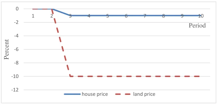
Finally, the mechanisms illustrated above would indicate the price trend decline would
[image:19.595.126.480.380.556.2]happen along with the shrinkage of worker population, and the value of the decline can be calculated from equations (26) and (27). Substituting in the parameters from the previous section, the trends of house/land price are shown in Figure 3, where their values decline by 1 percent and 10 percent, respectively.
Figure 3. Price Changes: Long-Term Effect of Fertility Rate Decline
Notes: The corresponding demographic changes are shown in Figure 1a.
5.2. Longevity Increase
As explained in the section on the solution method, the effect of an increase in longevity impacts on steady states instead of trends.
There are three ways of calculating the effect on steady states: derive the analytical solution, calculate the partial derivative from the above, or use numerical simulations when the above is not practical. The first two have proved difficult thus numerical simulations have been
-12 -10 -8 -6 -4 -2 0
1 2 3 4 5 6 7 8 9 10
Per
ce
nt
Period
19
employed. By using parameter values and the changes in longevity, this method permits the calculation of steady-state values for the endogenous variable.
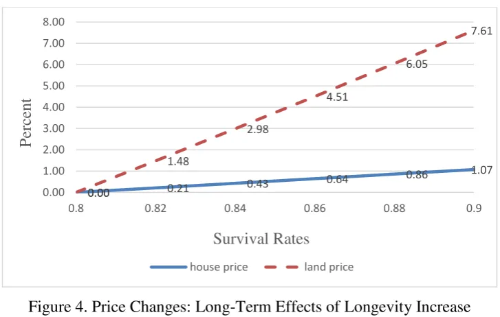
Here, by using the calibrated parameters and assumptions in the previous section, the numerical solution is presented to show the long-term effect of an increase in longevity. The
robustness of the results is checked as explained in Appendix D. The results of the numerical solution are shown in Figure 4. The effects of an increase in the survival rate from 0.8 to 0.9 are calculated and plotted in this figure: it shows a positive impact on price of an increase in longevity.
[image:20.595.121.485.336.567.2]This result indicates that, for plausible calibrations of the structural parameters of the economy, the long-term effects of an increase in longevity on the prices is positive. In addition, as shown in Figure 4, the rise in the price of land is higher than that of the house. Thus, for the given parameters, the long-term effect of an increase in longevity on land price is larger than that on the house.
Figure 4. Price Changes: Long-Term Effects of Longevity Increase
Notes: the survival rate is incremented by 0.1 to derive the corresponding steady state prices for house and land separately.
Result 2: the long-run effect of an increase in longevity is positive on both house and land
prices. Moreover, its effect on the land price is bigger than that on the house price.
5.3. Overall
We next investigate combined effects of a fall in the fertility rate and an increase in longevity. More concretely, when using the assumed demographic changes in the previous section, their overall effects on the prices are shown in Table 4.
0.00 0.21 0.43
0.64 0.86 1.07
0.00
1.48
2.98
4.51
6.05
7.61
0.00 1.00 2.00 3.00 4.00 5.00 6.00 7.00 8.00
0.8 0.82 0.84 0.86 0.88 0.9
P
erc
ent
Survival Rates
20
In the long run, the house price rises by 0.07 percent. This rise indicates that, conditional on the values of the assumed parameters, the positive effect on house price from an increase in longevity is greater than the negative effect from the fall in fertility. In contrast, the land price declines by 2.39 percent. Thus, the negative effect of the simulated fall in fertility outweighs
[image:21.595.76.523.202.260.2]the positive effect from the simulated increase in longevity.
Table 4—Prices Changes: Long-Term Effect of Aging Population (in percent)
effect of decline in fertility rate
effect of increase in longevity
overall effect
house price -1.00 1.07 0.07
land price -10.00 7.61 -2.39
Note: the numbers come from Figure 3 and 5, and the overall effect is the sum of the two. The justification of this method is shown in Appendix D.
These offsetting effects can be deduced from Result 1 and Result 2. Recall from Result 1, the long-term effect of fertility rate decline on prices is negative; however, in Result 2, the long-term effect on prices of an increase in longevity is positive. Because these two effects move in opposite directions, the net effect depends on which of the above is overwhelming. Furthermore, if we manipulate the extent of fertility rate decline, these opposing effects could
be studied more closely for specific parameter values.
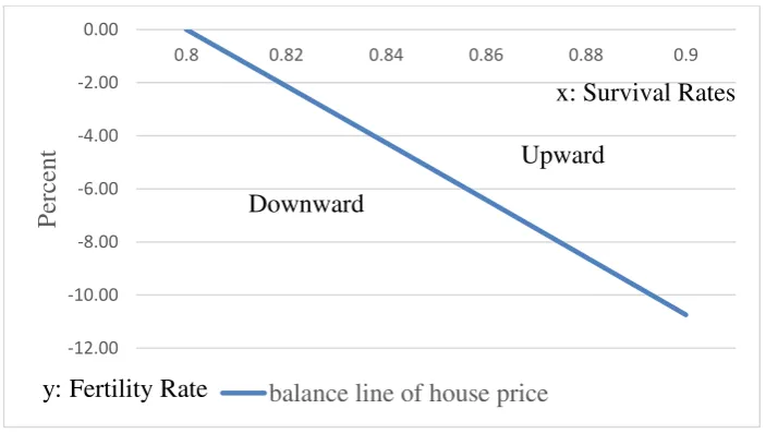
As shown in Figure 5, the Cartesian plane consists of the fertility rate decline (y-axis) and
longevity increase (x-axis). The line pictured in the plane is a set of points, denoting combinations of fertility rate decline and longevity increase. For house price, on this line, the upward effect from longevity increase equals the downward effect from fertility rate decline. That is, the net effect of an aging population on house prices is zero on this line.
Figure 5. Plane of Aging Population and Balance Line of House Price
Notes: The effect of longevity increase on house price comes from Figure 4, and the effect of fertility rate decline is calculated according to (26).
-12.00 -10.00 -8.00 -6.00 -4.00 -2.00 0.00
0.8 0.82 0.84 0.86 0.88 0.9
P
erc
ent
balance line of house price y: Fertility Rate
Downward
Upward
[image:21.595.127.479.517.721.2]21
Moreover, the line pictured in Figure 5 is also a dividing line. It divides the quadrant of the plane into two parts. On the right side of the line, the house price will rise in the long run, because of the stronger effect from an increase in longevity via-a-vis a fall in fertility. However, on the left side of the line, the house price will decline due to the weight of fertility rate decline.
[image:22.595.123.485.236.464.2]For land price, a similar plane is shown in Figure 6, together with a line, on which the long-term effect of aging population is zero. Similar to that of the house price, the quadrant is also divided into two parts by this balance line, and its right / left side would be the upward / downward area for the land price.
Figure 6. Plane of Aging Population and Balance Line of Land Price
Notes: The effect of longevity increase on land price comes from Figure 4, and the effect of fertility rate decline is calculated according to (27).
Figure 7. Plane of Aging Population and Balance Line of Land Price
Notes: source from Figure 5 and 7.
-8.00 -7.00 -6.00 -5.00 -4.00 -3.00 -2.00 -1.00 0.00
0.8 0.82 0.84 0.86 0.88 0.9
P
erc
ent
balance line of land price y: Fertility Rate
Downward
Upward
x: Survival Rates
-12.00 -10.00 -8.00 -6.00 -4.00 -2.00 0.00
0.8 0.82 0.84 0.86 0.88 0.9
P
erc
ent
balance line of house price balance line of land price
y: Fertility Rate
Downward
Upward x: Survival Rates
[image:22.595.119.486.500.720.2]22
Lastly, notice that the balance lines of house and land prices do not coincide with each other, which is shown in Figure 7. Thus, the zero long-run effect cannot be achieved for both the prices simultaneously. Moreover, the quadrant is divided into three areas by two different lines. Because the areas preserved the properties as in Figure 5 and 7, the right most area is where
both land and house prices rise while left-most region is where both prices fall. The middle area lends room for the two prices to diverge: specifically where the price of land drops while that for houses increase. The parameters assumed in the calculations are those for this specific region as shown in Table 4.
To sum up, the discussion above could be highlighted by the following result:
Result 3: the aging population could have zero effect on either house or land price in the
long run.
6. Simulation
In this section, we report on simulations of the economic effects of the demographic changes presented in Figure 1. Specifically, the simulations provide the dynamics in terms of household utility and housing prices during the transition periods. From these dynamics, we explain how the demographic changes and economic fluctuations are interconnected. The results have had trends involved according to (23). Thus, they are the overall dynamics of variables instead of steady states.
6.1. Households’ Utility
Aside from the negative utility from working, the household utility is determined by the non-housing consumption and house and land owned per capita. If we divide the households into
workers and retirees, their per capita utility is shown in Figure 8. The per capita consumption of workers is greater from that of period 1 in periods 2 to 4 (see Figure 8a) when workers own more houses and land both in the long run and short run (see Figure 8c, e). In contrast, the
23
Figure 8. The Utility Dynamics (per capita)
Note: the corresponding demographic changes are presented in Figure 1, both the fertility rate decline and longevity increase happen from period 2 to 3.
The results in Figure 8 show that, relative to period 1 (the original state), the utility of workers
is higher; however, the retirees’ utility is worse than their original state. We next discuss the retirees’ utility since workers’ behaviour is influenced by the expectations of their life in retirement.
24
During the transition period, the significant utility loss of retirees is due to the decline in the fertility rate. This decline leads to fewer workers and a concomitant rise in the proportion of retirees. Especially in period 3, the proportion of retirees would reach its peak (see Figure 1f), meaning that the pension income from workers would be shared by more retirees, leading to
the most drastic losses in utility. After that, this utility will rise along with a decline in the proportion of retirees (see Figure 1f), and move towards its long run level.
For the workers, their behaviour would be influenced by their expectations about the living standard of their retirement. In the long-run, the higher utility is due to the increased savings
of workers. Recall that the utility loss would happen in households’ retirement period, the workers with rational expectation would increase their savings to fund their retirement so as to maximize their life-span utility. Specifically, the households, having perfect foresight of their future utility loss, would purchase more house and land when they are workers, and sell them when they retire. This purchase behaviour against the future utility loss raises the house and land owned by workers and with it their utility.
During the transition period, the increased utility of workers comes from the fall in the fertility rate. Because of the fertility rate decline, the worker population decreases accordingly. However, the total income of workers will not decrease to the same extent. The key driver here
is the wealth stock of the firms, including 𝐾𝑐,𝑡−1, 𝐾ℎ,𝑡−1 and 𝐿𝑒,𝑡−1 (see equation (10) and (11)). When worker population declines, the adjustments of the wealth are not immediate, indicating higher per worker output in goods and houses. According to equation (16), higher per worker output and wealth stock translates into the income of workers through wages and profits. Thus, higher per capita income would accrue to workers, and their utility increases.
Along with the adjustment of the wealth stock, workers’ utility will tend to converge towards
its long run level.
Based on the discussion above, we note that an aging population would increase inequality across generations. The utility of workers increases whereas that of the retirees falls. Especially in the transition periods, this growth in inequality would be significant. In these periods, as has been illustrated above, the significant aging population and the wealth stock adjustment would drive a wedge between the two generations.
The results of this section can be concluded as follows:
Result 4: the aging population could increase inequality across generations. Specifically,
25
6.2. Prices
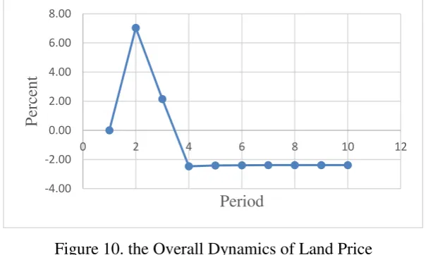
[image:26.595.153.453.184.375.2]The price dynamics following the demographic changes presented in Figure 1 is explained next. The house price rises from period 1 to 3, and then declines from period 3 to 4 (see Figure 9). Meanwhile, the land price also rises from period 1 to 2, and declines from period 2 to 4 (see Figure 10).
Figure 9. the Overall Dynamics of House Price
[image:26.595.151.455.412.593.2]Note: the corresponding demographic changes are presented in Figure 1, both the fertility rate decline and longevity increase happen from period 2 to 3. After that, the fertility rate moves back to the replacement level, while the longevity stays stable.
Figure 10. the Overall Dynamics of Land Price
Note: the corresponding demographic changes are presented in Figure 1, both the fertility rate decline and longevity increase happen from period 2 to 3. After that, the fertility rate moves back to the replacement level, while the longevity stays stable.
As shown in Figure 9 and 10, the land price dynamics produce a turning point at period 2, while the turning point of the house price happens at period 3. Before these points, the prices are rising; however, after these points, the prices fall. What is the mechanism that connects the
demographic change to the price movements?
To explain these dynamics, the Euler Equations of house and land are listed:
𝑞̃𝑡 = 𝛽𝐸𝑡(exp (𝑔𝑞,1+𝑡) 𝑞̃1+𝑡(1 − 𝛿ℎ)𝑐𝑐1,𝑡
2,1+𝑡) + 𝑗ℎ
𝑐1,𝑡
ℎ̃1,𝑡 (28)
-1.00 -0.50 0.00 0.50 1.00 1.50 2.00
0 2 4 6 8 10 12
P
erc
ent
Period
-4.00 -2.00 0.00 2.00 4.00 6.00 8.00
0 2 4 6 8 10 12
P
erc
ent
26
𝑝̃𝑙,𝑡 = 𝛽𝐸𝑡(exp (𝑔pl,1+t) 𝑝̃𝑙,1+𝑡 𝑐𝑐1,𝑡
2,1+𝑡) + 𝑗𝑙
𝑐1,𝑡
𝑙̃1,𝑡 (29)
, where the variables with a tilde denote their de-trended values.
According to (28) and (29), the price dynamics are explained by the utility changes of households, which are presented in Figure 8. In the first step, we will emphasize that the utility changes and perfect foresight of households are driving prices to rise from period 1 to 2.
As shown in Figure 8b, the per capita consumption of retirees would decline significantly from period 2 to 3. Given the assumption of perfect foresight of households, their behaviours would change accordingly and beforehand. The expected decline in consumption is denoted by
𝐸𝑡(𝑐2,1+𝑡). According to (28) and (29), the decline of 𝐸𝑡(𝑐2,1+𝑡) will raise the house and land
prices (𝑞̃𝑡 and 𝑝̃𝑙,𝑡) beforehand. Therefore, if the expected consumption decline would happen from period 2 to 3, then the price rises would precede period 2. This mechanism explains the price rise before the demographic changes.
Intuitively, as explained in the household utility section, expectations drive the price rise. When a decline in consumption is anticipated, the households raise their savings by purchasing more housing and land when they are workers (see figure 8c, e). It is these purchases which drive the price rise.
After period 2, the drop in the fertility rate tends to drag the prices down as discussed in the
previous section. Specifically, the house and land prices should be lowered by 1 and 10 percent respectively from period 2 to 3 in terms of the fertility rate decline (see figure 3). However, the
price dynamics show that the land price falls by 5 percent instead, and the house price even rises (see figure 9 and 10). What is the force supporting the prices?
Here, this force comes from the character of stock of wealth. As discussed previously, the stock of wealth would not adjust immediately against a decline in the population of workers. Therefore, with these wealth stocks, the per capita income of workers in period 3 rises. More house and land would be purchased by using these incomes, and these purchases are supporting the price of these assets. This supporting force shapes the price dynamics by preventing the land price from sharp decline and postponing the turning point of the house price.
Nevertheless, this supporting force fades away as the wealth stock is adjusted, and thus both
the prices fall at period 4. The fading of this supporting force can be reflected by the workers’
27
In particular, the land price reaches its long run level at period 4, but the house price overshoots (see figure 9 and 10). Why? This further decline of house price is explained from
changes in the house stock. To illustrate, we should notice that the house stock ℎ̃1,𝑡 is not adjusting simultaneously with the consumption (see Figure 8c). Because of the depreciation character of house stock, the adjustment would not be immediate, but take place gradually.
Based on (28), a higher ℎ̃1,𝑡 indicates a lower house price. Thus, in period 4, because ℎ̃1,𝑡 is higher than its long run level, the price would have a further fall. This mechanism enriches the discussion about overshooting phenomena that started with Dornbusch (1976).
In sum, connections between demographic changes and price dynamics are presented above, and these connections could be summarized by the following result:
Result 5: aging population could cause turning points in housing prices.
Although this result is based on the specific demographic changes presented in the previous section, it is theoretically grounded as shown in Figure 7– an issue under current investigation.
7. Conclusion
The effect of an aging population on housing prices remains an unresolved issue with mixed empirical findings. This debate began with Mankiw and Weil (1989) and has been ongoing since. Here we build an overlapping generations model where aging results from a combination of a decline in fertility and an increase in longevity to simulate effects of the above on housing prices. Our simulations for plausible parameter values give mixed results, depending on which of the above-mentioned overwhelms in terms of the impact of aging on house (and land) prices.
This paper has tackled the impact of aging on housing prices from a theoretical perspective. Our result provides reasons for the mixed results shown through empirical studies. It shows that a decline in the fertility rate depresses housing prices while an increase in longevity does the opposite – the net effect of a simultaneous change in the above two factors depends on
which effect is overwhelming. Note that aging is caused by a combination of a fall in fertility with an increase in longevity, but the exact magnitude of the afore-mentioned differs across contexts. More concretely, in the long run, housing prices will decline if the drag of a fall in fertility outweighs the push from an increase in longevity, and vice versa. This result may explain the mixed findings from existing empirical research.
28
the simulations and explained theoretically. Before the turning points, the prices would rise in anticipation of a longer life span by existing population of workers and thus the need for more wealth to fund retirement. Nevertheless, the decline afterwards is due to the decrease of worker population caused by the lower fertility rate. Although the wealth stock would temporary
support the housing prices, the price declines would continue when this support effect fades away.
Furthermore, household behaviour has also been discussed in this paper, and the analysis showed that the demographic changes would lead to welfare inequality across generations. More concretely, the utility of workers will be higher; however, that of retirees will be lower (see Figure 8). This inequality would be most significant during the transition periods.
29
Appendix A. per capita Version Model Equations
The per capita version model equations are transformed from the corresponding aggregate equations, and the derivation is based on Eq. (1), (2), (3) in the demography section.
Households: For each generation, the budget constraint is shown by variables in lower case
denoting per capita amount of that generation.
𝑐𝑡,1+ 𝑞𝑡ℎ𝑡,1+ 𝑝𝑙,𝑡𝑙𝑡,1= (1 − 𝑇)(𝑤𝑐,𝑡𝑛𝑐,𝑡+ 𝑤ℎ,𝑡𝑛ℎ,𝑡+ 𝑑𝑡) (𝐴1)
𝑐1+𝑡,2+ 𝑞1+𝑡ℎ1+𝑡,2+ 𝑝𝑙,1+𝑡𝑙1+𝑡,2=
𝑞1+𝑡(1 − 𝛿ℎ) (𝜋ℎ𝑡,1 1+𝑡+
𝜋𝑡ℎ𝑡,2
𝜋1+𝑡𝑛𝑡) + 𝑇(𝑑1+𝑡+ 𝑛𝑐,1+𝑡𝑤𝑐,1+𝑡+ 𝑛ℎ,1+𝑡𝑤ℎ,1+𝑡)
𝑛1+𝑡
𝜋1+𝑡
+𝑝𝑙,1+𝑡(𝜋𝑙ℎ,𝑡,1 1+𝑡+
𝜋𝑡𝑙𝑡,2
𝜋1+𝑡𝑛𝑡) (𝐴2)
Firms: For firms, the variables in lower case represent the amount per worker.
𝑦𝑡= 𝐴𝑐,𝑡 (𝑘𝑐,𝑡−1𝑛 𝑡 )
𝜇𝑐
𝑛𝑐,𝑡1−𝜇𝑐 (𝐴3)
ih𝑡 = 𝐴ℎ,𝑡 (𝑘ℎ,𝑡−1𝑛 𝑡 )
𝜇ℎ
(𝑙𝑒,𝑡−1𝑛
𝑡 ) 𝜇𝑙
𝑛ℎ,𝑡1−𝜇ℎ−𝜇𝑙 (𝐴4)
𝑘𝑐,𝑡 = (1 − 𝛿kc)𝑘𝑐,𝑡−1𝑛
𝑡 + ik𝑐,𝑡− 𝜙𝑐,𝑡 (𝐴5)
𝑘ℎ,𝑡= (1 − 𝛿kh)𝑘ℎ,𝑡−1𝑛
𝑡 + ikℎ,𝑡− 𝜙ℎ,𝑡 (𝐴6)
𝜙𝑐,𝑡 = 𝜙𝑐(𝑘𝑐,𝑡, 𝑘𝑐,𝑡−1) = 𝜙2 (𝑘𝑐 𝑘𝑘𝑐,𝑡𝑛𝑡
𝑐,𝑡−1 − exp (𝑔𝐾𝐶,𝑡)) 2𝑘
𝑐,𝑡−1
𝑛𝑡 (𝐴7)
𝜙ℎ,𝑡 = 𝜙ℎ(𝑘ℎ,𝑡, 𝑘ℎ,𝑡−1) =𝜙2 (𝑘ℎ 𝑘𝑘ℎ,𝑡𝑛𝑡
ℎ,𝑡−1− exp (𝑔𝐾𝐻,𝑡)) 2
𝑘ℎ,𝑡−1
𝑛𝑡 (𝐴8)
𝑑𝑡+𝐴𝑘𝑐,𝑡
𝑘,𝑡+ 𝑘ℎ,𝑡+ 𝑤𝑐,𝑡𝑛𝑐,𝑡 + 𝑤ℎ,𝑡𝑛ℎ,𝑡+ 𝑝𝑙,𝑡𝑙𝑒,𝑡+
𝜙𝑐,𝑡
𝐴𝑘,𝑡+ 𝜙ℎ,𝑡=
𝑦𝑡+ 𝑞𝑡 ih𝑡+1 − 𝛿𝐴 kc 𝑘,𝑡
𝑘𝑐,𝑡−1
𝑛𝑡 + (1 − 𝛿kh)
𝑘ℎ,𝑡−1
𝑛𝑡 + 𝑝𝑙,𝑡
𝑙𝑒,𝑡−1
30 Equilibrium:
𝑦𝑡 = 𝑐𝑡+ik𝐴𝑐,𝑡
𝑘,𝑡 + ikℎ,𝑡− 𝜙𝑡 (𝐴10)
ℎ𝑡 = ih𝑡+ (1 − 𝛿ℎ)ℎ𝑛𝑡−1
𝑡 (𝐴11)
𝑙𝑡= 𝑙ℎ,𝑡+ 𝑙𝑒,𝑡 (𝐴12)
, where 𝑐𝑡 = 𝑐𝑡,1+𝜋𝑡
𝑛𝑡𝑐𝑡,2, ℎ𝑡 = ℎ𝑡,1+ 𝜋𝑡
𝑛𝑡ℎ𝑡,2, 𝑙ℎ,𝑡 = 𝑙ℎ,𝑡,1+ 𝜋𝑡 𝑛𝑡𝑙ℎ,𝑡,2.
Appendix B. Trends
The proof of the algorithm
Proposition 1
For the linear equation (21), we have 𝐺1,𝑡= 𝐺2,𝑡= 𝐺𝑡 and 𝑔1,𝑡 = 𝑔2,𝑡= 𝑔𝑡. Proof
We will prove that the unequal trend growth rates cannot exist according to our assumptions. If not, then there are exogenous variable changes such that the growth rates are not equal. In this circumstance, we fix the exogenous change so that the unequal trend growth rates are constants, i.e. 𝐺𝑡 = (exp (𝑔))𝑡 > 0, 𝐺1,𝑡 = (exp (𝑔1))𝑡 > 0, 𝐺2,𝑡 = (exp (𝑔2))𝑡> 0 . The inequality implies that there are some growth rates smaller than the others. Without loss of
generality, we assume that 𝑔 ≤ 𝑔𝑖 and at least one of the inequality is strict13. We rewrite the equation (21) as follows:
𝑋𝑡
𝐺𝑡 = 𝑎
𝑋1,𝑡
𝐺1,𝑡
𝐺1,𝑡
𝐺𝑡 + 𝑏
𝑋2,𝑡
𝐺2,𝑡
𝐺2,𝑡
𝐺𝑡
𝑋̃𝑡 = 𝑎𝑋̃1,𝑡𝐺𝐺1,𝑡
𝑡 + 𝑏𝑋̃2,𝑡
𝐺2,𝑡
𝐺𝑡
𝑋̃𝑡= 𝑎𝑋̃1,𝑡(exp(𝑔exp(𝑔) )1) 𝑡
+ 𝑏𝑋̃2,𝑡(exp (𝑔exp(𝑔) )2) 𝑡
(𝐵1)
In equation (B1), at least one of the terms (exp (𝑔𝑖)
exp (𝑔))𝑡 would go infinity when 𝑡 → +∞.
Consequently, the steady state 𝑋̃𝑡 would become infinity if 𝑋̃𝑖,𝑡 are not zero. Either the way, it
13
31
violates the assumption one. Thus, for any exogenous change, we have 𝑔1,𝑡 = 𝑔2,𝑡= 𝑔𝑡 and
𝐺1,𝑡 = 𝐺2,𝑡 = 𝐺𝑡. #
Proposition 2
For the Cobb-Douglas form equation (22), we have 𝐺𝑡= 𝐺1,𝑡𝑎 𝐺2,𝑡𝑏 and 𝑔𝑡 = 𝑎 𝑔1,𝑡+ 𝑏 𝑔2,𝑡. Proof
The logic is the same as the proof of the proposition 1. Divide both sides of the equation (22) by 𝐺𝑡 and we derive the equation as follows:
𝑋̃𝑡= 𝑋𝐺𝑡 𝑡 = 𝑐
𝑋1,𝑡𝑎 𝑋2,𝑡−𝑖𝑏
𝐺𝑡 = 𝑐 (
𝑋1,𝑡
𝐺1,𝑡) 𝑎
(𝑋𝐺2,𝑡−1
2,𝑡 ) 𝑏𝐺
1,𝑡𝑎 𝐺2,𝑡𝑏
𝐺𝑡 = 𝑐𝑋̃1,𝑡
𝑎 ( 𝑋̃2,𝑡−1
exp (𝑔2,𝑡)) 𝑏
𝐺1,𝑡𝑎 𝐺2,𝑡𝑏
𝐺𝑡
If 𝐺𝑡≠ 𝐺1,𝑡𝑎 𝐺2,𝑡𝑏 , then there are exogenous variable changes satisfy this inequality. Similar to the proof in proposition 1, we fix the exogenous change and the unequal trend growth rates
would be constants. Then, the term 𝐺1,𝑡𝑎 𝐺2,𝑡𝑏
𝐺𝑡 will turn to zero or infinity when 𝑡 → +∞. To hold
the equation, the steady states would become either zero or infinity, and thus violate the
assumption one. Therefore, for any change in exogenous variables, we have 𝐺𝑡= 𝐺1,𝑡𝑎 𝐺2,𝑡𝑏 . Taking log-difference operation on both sides of 𝐺𝑡= 𝐺1,𝑡𝑎 𝐺2,𝑡𝑏 , we have:
𝑙𝑛𝐺𝑡− 𝑙𝑛𝐺𝑡−1 = 𝑎(𝑙𝑛𝐺1,𝑡− 𝑙𝑛𝐺1,𝑡−1) + 𝑏(𝑙𝑛𝐺2,𝑡− 𝑙𝑛𝐺2,𝑡−1)
According to equation (3), the above equation can be written as 𝑔𝑡= 𝑎 𝑔1,𝑡+ 𝑏 𝑔2,𝑡. # Remark 1
The conclusion in proposition 1 can be extended when there are more linear terms in equation (4), i.e. 𝐺𝑡 = 𝐺1,𝑡 = 𝐺2,𝑡 = ⋯.
Remark 2
The conclusion in proposition 2 can be extended when there are more terms multiplied in the
right-hand side of the equation (7). For example, when 𝑋𝑡= 𝑑𝑋1,𝑡𝑎 𝑋2,𝑡−1𝑏 𝑋3,𝑡−1𝑐 , we have 𝑔𝑡 =
𝑎 𝑔1,𝑡+ 𝑏 𝑔2,𝑡+ 𝑐 𝑔3,𝑡.
Remark 3
The relationship of the trend growth rates is contemporaneous, and thus the time subscript can be omitted.
So far, the algorithm that calculates balanced growth rates in literature is shown to be held in more general circumstance under the two assumptions we made.