Munich Personal RePEc Archive
An Agent Based Macroeconomic Model
with Social Classes and Endogenous
Crises
Russo, Alberto
Università Politecnica delle Marche
31 December 2016
Online at
https://mpra.ub.uni-muenchen.de/77175/
An Agent Based Macroeconomic Model with
Social Classes and Endogenous Crises
Alberto Russo
∗Universit`a Politecnica delle Marche
December 31st, 2016
AbstractThis paper proposes an agent based macroeconomic model in which income distribution and wealth accumulation depend on the role that agents play in productive activities, that is capitalists or workers. In this framework, social class dynamics underlie the endogenous process of firm formation. The focus is on the interplay between the evolution of social structure and macroeconomic dynamics and on how business cycles and crises may endogenously emerge as the result of the interaction between financial and real factors underlying the process of capitalist production.
Keywords: heterogeneous interacting agents; social structure, macroeconomic dy-namics, inequality, crisis.
JEL Classification Numbers: P10, D31, C63.
1
Introduction
This paper investigates the interplay between social structure and macroeconomic dynamics. In particular, the joint evolution of social classes, production and distribution is analyzed within a macroeconomic model with heterogeneous agents. The aim is to show how endogenous business cycles and crises may emerge from decentralized interactions among agents that self-organize in social classes along the process of capitalist production. As a result, highly unequal societies may develop even starting from perfect equality.
Inequality is an unavoidable feature of a capitalist economy, although its degree may vary depending on political choices. The distribution of income and wealth is related to how the society is organized and the associated level of inequality shapes macroeconomic evolution. In particular, increasing inequality may result in a lack of aggregate demand that, in turn, may reduce the profit rate of productive firms, with a consequent negative impact on bank profits due to the contagion of financial distress (e.g. bankruptcy chains); moreover, the decline of the profit rate may impact the “social relations of production”, with further macroeconomic effects.
As for the methodology, the paper proposes a agent based macroeconomic model with an initial population of homogeneous agents that differentiate along time, thus becoming heterogeneous particularly due to the role they play in productive activities, e.g. capital-ists or workers. As we will see below, for an agent, belonging to one or another social class depends on a wealth-related stochastic process which is also shaped by the evolution of the profit rate. Therefore, the model is characterized by an endogenous process of class division that, in turn, shapes the co-evolution of production and distribution. Moreover, social class dynamics are also at the root of the process of firm formation, though in a simplified setting in which one capitalists can hire one or more workers, giving rise to a firm. In general, then, this paper proposes a combination of theold theoretical tradition of Classical economists and the new methodology of agent based modelling.
2
Related literature
In this section we briefly review the literature on three main topics, on which the subsequent model is based, that the paper tries to merge in order to analyze the co-evolution of production, distribution and social structure in a macroeconomic setting with heterogeneous interacting agents.
2.1
Agent based modelling in macroeconomics
In recent years, there has been a blossoming of agent based macroeconomic models, especially in Europe. In what follows a few examples are provided regarding the most recent papers.
A large-scale model carried out in the EURACE European project is described in Dawid et al. (2013): this is an agent based stock flow consistent framework for macroe-conomic analysis.1
Within the same project other versions have been developed, as for instance Cincotti et al. (2010); this model has been used to analyze the impact of debt and deleveraging on macroeconomic performance (Raberto et al., 2012), the effectiveness of the banks’ capital adequacy regulation (Teglio et al., 2012), and the role of macropru-dential policies (Cincotti et al., 2012); moreover, the same agent based macroeconomic model has been employed to analyze the mortgages market and housing bubbles dynamics (Erlingsson et al., 2014). An empirically grounded agent based model of housing boom and bust and systemic risk has been proposed by Geanakoplos et al. (2012). An extension of the EURACE framework including housing market dynamics is proposed in van der Hoog and Dawid (2015).
Dosi et al. (2013) studies the relationship between income distribution and mone-tary/fiscal policies based on a previous agent based macroeconomic model that, com-bining Keynesian and Schumpeterian features, finds strong complementarities between factors influencing aggregate demand and drivers of technological change that affect both short-run fluctuations and long-term growth patterns (Dosi et al., 2010). This framework has been further extended in Dosi et al. (2015) to identify the most appropriate combi-nation of fiscal and monetary policies in economies subject to banking crises and deep recessions.
Built on previous works as Russo et al. (2007) and Riccetti et al. (2013a), Riccetti et al. (2015) proposes a macroeconomic model with heterogeneous agents, that directly interact in different markets according to a common decentralized matching mechanism, showing that business cycles as well as extended crises endogenously emerge due to the interplay between real and financial factors; the model has been employed to analyze the
1
role of unemployment benefits (Riccetti et al., 2013b), the effects of the financialization of non-financial corporations (Riccetti et al., 2016), the effectiveness of financial regulation (Riccetti et al., 2017), the consequences of growing inequality (Russo et al., 2014), and the relationship between household debt, financial fragility and crisis episodes triggered by income and wealth distribution dynamics (Russo et al., 2016).
Combining some features of above papers, particularly the centrality of innovation dynamics in Dosi et al. (2013) and the importance of financial fragility and default conta-gion in Riccetti et al. (2015), Caiani et al. (2016) develop an agent based macroeconomic model, in which both micro and macro variables are stock flow consistent, to analyze the behaviour of business cycle fluctuations and replicate a variety of micro-meso-macro stylized facts.
proxy of sector profitability, thesocial structureis exogenous. The present paper wants to overcome this limitation by assuming that each agent can potentially play different roles in productive activities; therefore, in each period of time, depending on the conditions we will analyze below, an agent can act as a capitalist or as a worker, thus resulting in an endogenous social class structure that affects economic performance and it is affected in turn. What the paper proposes, then, is a macroeconomic model with heterogeneous agents that self-organize in social classes.
2.2
Endogenous firm formation and social classes
According to Axtell (1999), firms emerge as cooperative teams under increasing re-turns in a population of agents that have preferences for both income and leisure time: within each group the output is divided into equal shares; each agent periodically adjusts its effort level to maximize utility non-cooperatively. Agents are allowed to join other firms or start up new firms when it is welfare-improving to do so. As a firm becomes large, agents have little incentive to supply effort, since each agent’s share is relatively insensi-tive to its effort level, thus giving rise to free-riders; as free-riding becomes commonplace in a large firm, agents migrate to other firms and the large firm declines. Moreover, firm size distribution tends to a power law under a continuous process of firm entry and exit. This is an empirical fact that validates the main finding of the model.
One of the central assumption in the above paper is that firm’s output is equally divided among team participants. This is not the usual distribution of the surplus created in a capitalist firm. Obviously, this is not the case because different agents have different roles and their remuneration is set accordingly. Moreover, when agents play different roles, the workers’ supply of effort can be monitored by the entrepreneur (in a small firm) or by managers (for larger firms). However, large firms – that present dynamic advantages due to economies of scale – can exhibit a static inefficiency due to the increasing number of layers of managers needed to control people working in the firm (Ciarli et al., 2010). Why then is it convenient to manage a (large) firm instead of performing a set of private market buying-selling transactions that reproduce the same activity?
That is a matter of power (Bowles and Gintis, 2008) and, in particular, the “right to manage” productive activities. In a sense, a firm can be considered as a “command economy”(Coase, 1937) in which the manager has the right to decide (and control) what the workers will do. In a competitive economy, then, many transactions are not market exchanges via prices, when instead operations within firms. According to the Simon (1951)’s model, indeed, under certain conditions an employment contract is preferred to a sales contract, giving the manager the authority over workers to organize the production and maximize firm’s profit.
is which role an individual plays within the firm and on which factors this depends. Ac-cording to Classical economists, the society is organized in classes that are characterized by a “conflict of interests” in the capitalist process of production and distribution. How do social classes emerge? Axtell et al. (2007) propose a multi-agent bargaining model in which social norms endogenously emerge based on decentralized interactions of many in-dividuals. In particular, the presence of a distinguishing “tag” (e.g., light and dark, that is a tag which can be completely meaningless, so that different individuals are identical in competence) can affect agents’ play when recognize a type or another as an opponent in the bargaining process; as a result, different bargaining behaviours can emerge among agents with respect to diverse partners and classes endogenously emerge.
However, being the manager or playing the capitalist role in productive activities is not a random outcome, nor it can be just the consequence of recognizing a “tag” (though this can be sufficient to generate different classes), when instead the consequence of material conditions of the individual as well as of the society. In particular, the individual choice of becoming a capitalist can be constrained by the amount of wealth an agent can invest in the productive activity: the larger the individual wealth the higher the probability to become a capitalist. The availability of external finance and credit rationing (Stiglitz and Weiss, 1981) may amplify this selection mechanism. Therefore, the crucial constraint to become an entrepreneur is the lack of capital, as suggested by Blanchflower and Oswald (1998). In other words, raising the necessary capital is the main problem in order to become an entrepreneur: if not enough capital is owned by an agent, and/or external finance is not available, the agent will play the worker role. According to Marx, the “social relations of production” in a capitalist economy are based on the employee-employer relationship and, according to Wright (2005, 2009), these relations can be considered as part of the microfoundations of macroeconomics: a small class of capitalist has the economic means to hire a large class of workers to be employed in productive activities performed in firms. The present paper proposes a simple mechanism of firm formation based on social class dynamics along these lines.
2.3
Stochastic processes and income/wealth distribution
“Since Pareto, it has long been known that the tail of distribution of income or wealth
w universally obeys a power-law distribution w−α for a constant α around 1.5− 2.5.
law in the right tail may emerge.
Levy (2003) introduces a reflective lower bound to a multiplicative process, within a stochastic model of wealth accumulation by financial investments, in order to study under which conditions the system converges to the empirically observed Pareto wealth distribution (Pareto, 1897). Based on multiple simulations of the model, “it seems that any stochastic multiplicative wealth accumulation model which assumes even a mild de-gree of differential investment talent leads to a distribution of wealth which is inconsistent with the empirical Pareto distribution” (Levy, 2003, p. 56). The main result is that Levy (2003)’s model replicates the empirically observed Pareto distribution for the high-wealth range, under the condition that the abilities of agents are homogeneous. Indeed, when abilities are heterogeneous, the model no longer converges to a power law tail, suggesting that in this framework the high inequality of wealth distribution is mainly due to chance
rather than differential abilities. “The result of this paper does not mean thatonly luck matters, and that any investment strategy is as good as any other. On the contrary, it means that one must apply his investment skills just in order to have a fair chance in the competition with other investors. Our findings suggest that because investors in the high-wealth range seem to have similar investment talents, at the margin it is only luck that differentiates between them” (Levy, 2003, p. 58). However, this model studies only top income dynamics for which the power law characterizes the “fat” right tail of the distribution. In other words, the author confined the analysis to wealth levels larger than
ˆ
ψ, maintaining that the wealth of individuals in the high-wealth range typically changes due to capital investments, leaving out of the analysis labour income (which is typically an additive rather than a multiplicative process), that is the main factor affecting wealth accumulation at the middle-to-lower range.
An extension of the Levy (2003)’s model has been proposed by Nirei and Souma (2007) by including also the labour income in the stochastic process of wealth accumulation. They propose a two-factor model in which asset returns are generated by amultiplicative
process, while wages depend onadditive process. Thus, they extend Levy (2003)’s results by adding to the power law tail for the high-wealth range the exponential decay for the low-wealth range, in line with Dragulescu and Yakovenko (2001)’s findings. Empirically, “the data analysis of income distribution in the USA reveals the coexistence of two social classes. The lower class (about 97% of population) is characterized by the exponential Boltzmann-Gibbs distribution, and the upper class (the top 3% of the population) has the power-law Pareto distribution” (Banerjee and Yakovenko, 2010, p. 9).2
By assumption that an agent is either an employee or an employer, Russo (2014) proposes a model in which agents either gain a capital income (i.e., a profit as the
2
An alternative approach has been proposed by Clementi et al. (2010) for which, instead of combining two different distributions, a (three-parameter)κ-generalized distribution is used to describe the whole
result of a multiplicative playing the capitalist role) or a labour income (i.e., a wage as the result of an additive process playing the worker role). As in Nirei and Souma (2007), this paper analyzes both the high-wealth range and the middle-low one; by considering class division, this model also studies the continuous inflows and outflows of agents from and to different classes. The aim is to discover the conditions, i.e. a large space of parameter combinations, under which richer individuals are more “powerful” than poorer ones in accumulating wealth, even starting equal initial endowments and homogeneous abilities. Moreover, this paper investigates the relation between class division and income/wealth inequality by applying a maximum likelihood esti-mation procedure to the wealth distribution for detecting the existence of a power law tail.
The present paper aims at extending the modelling framework proposed in Russo (2014) by plugging an endogenous social structure, that is a wealth-based class division process (subsection 2.3), into an agent based macroeconomic framework (subsection 2.1), where also the endogenous process of firm formation depends on social class dynamics (subsection 2.2).
3
The model
3.1
Model setup
In this section the structure of the model is presented. The economy is composed of
N agents, a banking sector,3
the government and the central bank. When referring to all theN agents the index i is used as a subscript, while the indexesk and j indicate an agent in the role of capitalist or worker, respectively.
The story begins with the government hiring some public workers by injecting an initial amount of public expenditure in the system (the central bank prints the money corresponding to government spending). At the beginning, all agents (including the banking system) have no income and no wealth; therefore, there are also no liabilities in the system (but for public debt financed by the money printed by the central bank). In each subsequent period, every agent has a probability to become acapitalist that depends on its relative wealth and the (past) average profit rate. This process gives rise to a social structure that shapes economic evolution (and vice versa).
In a monetary production system, as the simple economy we are describing, capitalists aim at making a monetary profit by hiring workers, producing and selling consumption goods to household and the public sector. In other words, we assume that production
3
regards only consumption goods and that only labour is used as an input.4
The banking sector finances production through loans and receive deposits from households. The central bank sets the policy rate (reacting to inflation and unemployment) and interacts with the banking sector through providing cash advances or receiving bank reserves. In order to keep under control the behaviour of public finances, tax rates evolve according to some fiscal rules. In what follows, the details of the model are explained.
3.2
Behavioural rules and interaction mechanisms
3.2.1 Consumption
The desired consumption of agent i at timet is based on the following equation:
ci,t =cmint +cy yi,t−1−cmint
+cωωi,t−1 (1)
where y represents past (net) income and ω is accumulated (net) wealth, cy and
cω are the propensity to consume out income and out of wealth, respectively, and
cmin
t = cmin ·(1 + ˙pt−1), with ˙pt−1 representing the past inflation rate; hence, agents calculate a consumption level based on both income and wealth, as well as on mini-mum consumption cmin
t . According to this assumption, there are not differences in the
consumption behaviour for agents belonging to different classes; indeed, differently from post-Keynesian models in which typically capitalists have a higher propensity to save than workers, we assume that the propensities to consume are constant and fixed across agents.5
Nevertheless, consumption inequality can characterize model dynamics given income and wealth inequalities which endogenously emerge from agents’ interaction and the social evolution of class structure.
3.2.2 Social classes
Agent i’s probability to play as a capitalist at timet depends on (after consumption) relative wealth and an adjustment factor related to the (past) profit rate, according to the following rule:
• firstly, a random number is picked from a (0,1) uniform distribution; if this number is smaller than the parameterλ, then the next steps are taken; otherwise, the agent does not change her status during period t;
4
Obviously, the next step for modelling a more realistic capitalist system is to introduce physical
capital in the production process. For now only working capital enters production.
5
• the variable bk for each agent at time t is calculated as follows:
bki,t = 1−(ˆωmaxt −ωˆi,t)/(ˆωmaxt −ωˆtmin) +κ πtr−1−bdt−1
. (2)
where ˆωmax
t and ˆωmint are, respectively, the maximum and the minimum value of
the wealth distribution at time t, ˆωi,t is the agent i’s wealth net of consumption
expenditure,πr
t−1 is the past rate of profit, bdt−1 is the ratio between bad debt and overall credit, and κ >0 is a parameter;
• a new variable ¯bki,t is computed by imposing 0 and 1 as the lower and upper bound
of bki,t, respectively.
• the individual variable rni,t is set by picking a number at random from a uniform
distribution U(0,1).
• finally, if ¯bki,t > rni,t, then agent i is a capitalist at timet.
For the sake of simplicity, it is assumed that such a stochastic rule is performed in each period of time; in principle, then, an agent could continuously change her role as time elapses, though the parameter λ introduces a certain degree of persistence.6
It is worth to note that, even in such a simplified framework, if playing as capitalist tends to result in higher incomes (than those gained by acting as a worker), thus wealth accumulation may lead to lower social mobility and the emergence of a restricted and relatively stable capitalist class, because of a wealth-based reinforcement mechanism.
3.2.3 Production plans and demand expectations
Capitalistkinvests a fraction of her (after consumption) wealth, ˆωk,t, in the productive
activity with the aim of obtaining a final wealth, ωk,t+1, larger than the initial one, ωk,t,
by producing and selling commodities, qk,t. According to the known scheme: ωk,t –qk,t –
ωk,t+1,ωk,t+1 should turn out to be larger thanωk,t when the goods market closes. Agent
k’s capital invested at timet in her firm is equal to
ak,t =α ωˆk,t (3)
where 0 < α < 1 is a parameter.7
The amount of wealth (1−α) ˆωk,t is retained by
the capitalist as a buffer that can be used as a collateral against the credit provided by the banking sector.
6
By contrast, one could assume that an agent plays a role until a certain condition holds: for instance, until a firm operates with a positive net worth, the agent financing that firm continues to play the capitalist role; then, the exit condition could be the firm default.
7
Based on demand expectations and labour demand, either self-financing production or a demand for bank loans will emerge. In particular, demand expectations depend on the aggregate quantity of goods sold in the previous period, Qt−1, and each capitalist expects to face a market share that depends on her invested wealth, ˆωk,t, relative to total wealth
invested; the latter is proxied by the total wealth invested in the previous period, ˆΩt−1, augmented by the inflation rate, ˙pt−1; accordingly, the quantity of goods the capitalist k expects to sell in periodt is:
qd
k,t=Qt−1·sharekt−1 (4)
This means that agents simply expect to face the same quantity of aggregate demand as in the previous period, Qt−1, to be divided by the same share of capitalists,sharekt−1. In order to produce the quantity of goods capitalists expect to sell, they have to assume workers to be employed in the production process. Assuming that production is a linear function of the number of workers to be hired by each firm, firm k’s labour demand is given by8
ld k,t=
qd
k,t/φ
(5)
where φ >0 is a parameter.9
Given the labour demand and the price of productive inputs, i.e. the wage rate w, capitalist k computes the total financing of production as follows:
abk,t =ldk,t·wt−1(1 + ˙wt−1) (6)
where it is assumed that expected value of the wage rate at time t is given by the past wage rate, wt−1, updated by considering the past wage inflation rate, ˙wt−1.
3.2.4 Self-financing and bank credit
Given total financing and the amount invested by each capitalist, production can either be (fully) self-financed or (partially) depend on bank credit. Therefore, if the capital invested by the k-th capitalist, that is ak,t, is smaller than total financing, abk,t,
then capitalist k’s demand for credit is given by
bd
k,t =abk,t−ak,t (7)
8
The discrete number of workers to be searched on the labour market is calculated by rounding the result in Equation 5.
9
Otherwise, the capitalist is able to self-finance production and then no credit is de-manded to the banking sector. Moreover, if capitalist k’s invested capital is larger than total financing, then the difference is deposited in the banking sector.
For those capitalists requiring external finance, i.e. when bd
k,t >0, the credit provided
by the banking sector is set as follows:
bk,t =min{bdk,t, β[(1−α)ˆωk,t]} (8)
where 0 < β < 1 is a parameter which represents the loan-to-value ratio. Therefore, the effective credit a firm k can receive from the bank is constrained by the availability of a collateral that is represented by the capitalist k’s wealth non invested in the firm; in case of default, the bank receives that amount and an endogenous recovery rate (RR) can be computed. Depending of the value of RR, the bank has to write down a “bad debt” in its balance sheet (as we will further analyze below).
The bank sets the interest rate on the loan provided to the capitalist k at time t by charging a risk premium which depends on firm k’s leverage, according to this equation:
rk,t = ¯rt+
q
1 +ρ bk,t/ak,t+ bdt−1−1 (9)
where ¯rt is the policy rate set by the central bank (see below for details), ρ > 0 is a
parameter, and bdt−1 is the previous period ratio between bad debt and overall credit.
3.2.5 Labour market
When the labour market opens, the government hires a fraction 0 < g < 1 of the population as public workers, among them not selected to play the role of capitalists at time t. The remaining workers and capitalists meet in the labour market according to a decentralized matching mechanism.
In each period the following interaction protocol takes place:
• a randomized list of unemployed workers is set;
• the first agent on the list, say the agent j, selects all the firms that have enough money to pay her desired wage wd
j,t and chooses one of those at random, say the
firm k; thus worker j gains the wage wd
j,t and the firm k’s wage bill is updated
accordingly; in the case there are no feasible matchings, i.e. if agent j’s desired wagewd
j,t is larger than firms’ available funds for hiring workers, then the worker j
remains unemployed at time t;
• at the end of the process, the unemployment rate can be computed, also including agents that, though selected as capitalists, were unable to hire workers in the labour market; each firm ends up with certain number of workers,lk,t ≤lk,td , that is equal or
smaller than labour demand (thus unfulfilled vacancies can result from the matching process); the k-th firm’s wage bill wbk,t is given by the sum of wages paid to hired
workers.
Workers pay a proportional tax on wage given by the tax ratetw. Unemployed people
receive a benefit from the government: ubj,t =σwt, where wt is the average paid wage at
time t, and σ >0 is a parameter.
When the labour market closes, workers update their desired wage based on (past) inflation and employment status; for the generic worker j:
wd j,t+1 =
wj,t·(1 + ˙pt+U(0,1)), if i employed at time t
wj,t·(1 + ˙pt−U(0,1)), if i unemployed at time t
(10)
where U(0,1) is a uniformly distributed random number between 0 and 1. As for capitalists, they also update their desired wage for the next period by only considering inflation; then, for the generic capitalist k: wd
k,t+1 =w
d
k,t·(1 + ˙pt).
There is a minimum level of the desired wage for each individual which is equal to:
wd
i,t+1 =σ < wt−1 >, where< wt−1 >is the average wage paid to workers.
3.2.6 Production, price setting and corporate profits
Firms produce homogeneous consumption goods by using only labour as input, i.e. the workerslk,t hired in the labour market, according to a linear production function with
productivity, φ >0, constant across firms and along time:
qk,t =φ lk,t (11)
The price of consumption goods, pt is set a according to the following rule:
pt=ADt/Qt (12)
whereADtis the monetary flow of aggregate demand and Qt is aggregate production,
that is the sum of firm’s output. Accordingly, each firm sells its output at the price pt.
Therefore, firm k’s profit is equal to
πk,t =ptqk,t, −wbk,t−rk,tbk,t (13)
3.2.7 Saving and wealth
The main source of saving is given by the remaining part of agents’ income after consumption. There are also two other components: (i) the part of invested wealth that capitalists do not employ in the productive activity (for instance, when the number of hired workers is below the labour demand); (ii) forced saving (for instance, due to goods market mismatch). Voluntary or involuntary saving is deposited in the bank, Dt, but
they do not receive remuneration.
At the end of each time period, agents update their wealth by adding to past wealth the income they gained either as worker (net wage or the unemployment benefit) or capitalist (net profit or unemployment benefit), the income deriving from saving and dividends (if distributed by the bank; more details on this below). In some cases, a default can result if wealth becomes negative. In the case of a firm going bankrupt, a non-performing loan arises that impacts the bank’s capital. The defaulted agent will start next period with zero wealth.
3.2.8 Banking sector
The profit of the banking sector is given by interest on firm loans, interest on gov-ernment bills (see below for more details), interest on reserves at the central bank minus interest on deposits, interest on cash advances provided by the central bank, and non-performing loans.
The bank pays a proportional tax on positive profits based on the tax rate tπ. If
financially sound, the banking sector distributes a fraction of net profit to agents, pro-portionally to their wealth. The percentage of profit to be distributed is by assumption equal to 1/2.
At the end of the time period, the banking sector updates its net worth by summing up current profit (net of tax and distributed dividends). In the unlikely case in which bank’s net worth turns to be negative, the government intervenes through a bank bailout. As for the relationship between the banking sector and the central bank, if the assets (i.e., firm loans and government bills) are larger than liabilities (i.e., deposits and net worth), then the difference is deposited at the central bank as a bank reserve (on which the bank receives an interest given by applying a markdown to the policy rate, ¯rt); in
the opposite case, the banking system receives cash advances from the central bank (on which the bank pays ¯rt).
3.2.9 Policy makers
The central bank either provides money (cash advances) or receives reserves depending on the banking sector’s balance sheet and sets the policy rate ¯rtaccording to the following
¯
rt=max{0, r∗+ ˙pt−1+ [θ′( ˙pt−1−p¯˙) +θ′′(¯u−ut−1)]} (14)
wherer∗ is the long-run policy rate, while θ′ and θ′′ represent, respectively, the weight
of inflation and unemployment in the monetary policy rule.
Government deficit is given by public expenditure for buying goods, payment of wage to public workers, unemployment benefits, interest on government bonds, in the extreme case of private bank defaults, bailout expenses; to these expenditures, revenues from taxing wages, profits and interest have to be subtracted. The public sector can issue government bonds on which it pays an interest whose spread on the policy rate, rs
t,
depends on the public debt-to-gdp ratio, that is µ, as follows:
rs t =γ(
p
1 +µt−1) (15)
where γ >0 is a parameter.
Tax rates evolve according to the following fiscal rules that aim at controlling the dynamics of both public deficit and debt over nominal gdp. Let consider the tax rate on wage, tw:
τw t =
min{1, τw
t +δ·U(0,1)}, if µt>µ¯ orνt>ν¯
max{0, τw
t −δ·U(0,1)}, otherwise
(16)
where νt is the public deficit-to-gdp ratio, while ¯µ and ¯ν represent, respectively, the
threshold for public debt and deficit over gdp. The same holds for the other tax rates.10
3.2.10 Aggregate variables
Aggregate variables are obtained by summing up individual variables: for instance,
Qt=Pkqk,t is aggregate production at timet. The price levelPtis given by the weighted
average of prices set by single firms (the weight being produced output). The interest rate on loans rt is also a weighted average across firms. Moreover, we compute other
statistics, as for instance the Gini index for consumption, income and wealth, in order to analyze the dynamic behaviour of the economic system.
4
Dynamics
Model dynamics are studied by means of computer simulation. First of all, the typ-ical behaviour of the model is described by presenting and commenting the output of a single run of the baseline scenario. Parameter values for the baseline model are presented
10
Table 1: Parameter setting
N number of agents 1000
κ class formation parameter 0.1
φ firm productivity 3
cy propensity to consume income 0.8
cω propensity to consume wealth 0.2
α wealth buffer parameter 0.25
β loan-to-value ratio 0.75
ρ interest rate parameter 0.1
g % of public workers 1/5
σ unemployment benefit parameter 0.1 ¯
υ public deficit threshold 0.03 ¯
µ public debt threshold 0.6
γ spread parameter ρ/2
δ tax adjustment 0.1
r∗ Taylor rule (TR) parameter 0.03
θ′ inflation weight in the TR 2
θ′′ unemployment weight in the TR 1
¯˙
p inflation target 2%
¯
u unemployment target 15%
in Table 1. Afterwards, multiple simulations are performed in order to collect statistics about model dynamics when starting from different seeds of the pseudo-number gener-ation process and then computing averages and dispersion measures of model variables across repetitions. Next step is a sensitivity analysis for investigating the impact on model dynamics of changing one parameter at time (thus keeping unchanged the other parameters). Finally, a Monte Carlo analysis is performed to explore model dynamics under different configurations of the parameter space.
4.1
Initial conditions
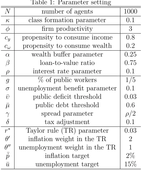
0 20 40 60 0
500 1000 1500
aggregate output
0 20 40 60 0
0.05 0.1 0.15 0.2 0.25
capitalist class size
0 20 40 60 0
1 2 3
gov deficit
0 20 40 60 0
0.2 0.4 0.6 0.8 1
[image:18.595.143.453.79.347.2]unemp rate
Figure 1: Simulations: 1000 agents, initialization phase
the reduction of unemployment.
4.2
A single run
100 150 200 250 300 500
1000 1500
aggregate output
100 150 200 250 300
0 0.1 0.2 0.3 0.4
unemp rate and wage share
100 150 200 250 3000.5
0.55 0.6 0.65 0.7
100 150 200 250 300
0 0.01 0.02 0.03 0.04 0.05 0.06
policy rate and interest rate
100 150 200 250 3000.04
0.05 0.06 0.07 0.08 0.09 0.1
100 150 200 250 300
0 0.2 0.4
capitalist class size
100 150 200 250 300
0.2 0.3 0.4 0.5 0.6 0.7
firms and bank profit rates
100 150 200 250 3000
0.02 0.04 0.06 0.08 0.1
100 150 200 250 300
0 0.5 1
income and wealth inequality
100 150 200 250 300
1 2 3
real wage and wage inflation
100 150 200 250 300−0.5
0 0.5
100 150 200 250 300
−0.5 0 0.5
gov deficit and debt
100 150 200 250 3000.4
0.6 0.8
100 150 200 250 300
0.2 0.25 0.3 0.35 0.4
tax rate and inflation rate
100 150 200 250 300−0.2
[image:19.842.166.708.97.454.2]−0.1 0 0.1 0.2
Figure 2: Simulations: from t=101 to T = 300
4.3
Multiple simulations
In oder to understand the statistical properties of the model we repeatedly simulate it with the parameters set as in Table 1. In 33 out of 50 replies the model remains in a “corridor of stability”, while in the remaining cases it gives rise to a large crisis without showing a self-correcting mechanism able to restore the stable path. In particular, when the aggregate demand becomes too low with respect to production, a large crisis follows and the private economy is disrupted. In simulations without large crises a typical business cycle emerges based on the conflictual relationship between social classes. These simulations are characterized by an average unemployment rate slightly above 20 %,11
an average profit rate of the corporate sector of more than 77 %, an inflation rate of about 1 %, a wage share equal to 60 %, a share of capitalists around 20%, and a Gini index for wealth inequality equal to 0.4143. In the next subsection we deepen the analysis of the statistical properties of the model by focussing on the effects of an important parameter on simulation results.
4.4
Sensitivity analysis
We perform a battery of computational experiments to analyze the sensitivity of model simulations to changing value of the parameterσ, that is the parameter governing unem-ployment benefits, which is particular important in that it influences the economic power of workers against capitalists in appropriating a larger share of the produced output. The baseline scenario has been described in the previous subsection and is characterized by a value of the parameter equal to 0.1. The lowest value we explore is 0.05 which gives rise to 32 out of 50 simulations with no large crises. In this case the average unemployment rate is almost 22 %, that is higher than whenσ = 0.1, the corporate profit rate is slightly higher than 80 %, an inflation rate lower of 0.4 %, a wage share of 60%, a share of capi-talists of alomost 18%, while the Gini index for wealth inequality is almost 0.47. In this case, than, compared to the baseline scenario, more inequality is due to a more restricted class of capitalists which benefits from a higher profit rate, though the economic system is more fragile and crisis prone. Therefore, a labour market characterised by a weak working class results in a higher profit rate (and more inequality) at the cost of more system instability.
Let’s now consider 50 simulations of the model when σ = 0.15. A higher value of the unemployment benefit level reduces the number of simulations showing a disrupting crisis: in this case, in 39 out of 50 simulations there are no large crises and the statistical properties of the model are the following: the unemployment rate is 19 %, the corporate profit rate is 78%, the inflation rate 1.6%, the wage share around 59 %, the share of the
11
capitalist class is 21 %, and Gini index for wealth is 0.3815, then showing a reduction of inequality.
If we continue to increase the parameter value, for instance for σ= 0.2, the frequency of large crises reduces: indeed, in 41 out of 50 simulations no large crises are observed. As for the main variables, the unemployment rate is almost 18%, corporate profit rate is higher than 80%, the inflation rate 2%, the wage share around 58%, the share of the capitalist class is higher than 22 %, and Gini index for wealth is 0.3586. Simulation results show that larger unemployment benefits result in lower unemployment, higher profits, a larger capitalist class and then lesser wealth inequality.
Another step in the sensitivity analysis exercise leads to a parameter value of 0.25. In this case the number of simulation without disruptive crises is 43 (out of 50), the corresponding unemployment rate is lower than 17%, the corporate profit rate is higher than 81%, the inflation rate 2.4%, the wage share around 58%, the share of the capitalist class is higher than 23 %, and Gini index for wealth is 0.3388. The same comments as in the previous paragraph apply.
When σ = 0.3, the simulations without large crises are 44 (out of 50), the unemploy-ment rate is around 16.5%, the corporate profit rate is higher than 80%, the inflation rate 2.6%, the wage share around 58%, the share of the capitalist class is higher than 23.5 %, and Gini index for wealth is 0.3249. Therefore, by increasing the unemployment benefit parameter a little bit more, similar effects are obtained but of minor magnitude.
If we fix the unemployment benefit parameter at a value of 0.35, the number of simulations with no large crises is equal to 6 (out of 50) and this suggests that now the level of unemployment benefit has become “excessive”. The average unemployment rate in the six simulations is 16%, the corporate profit rate is larger than 82%, the inflation rate 3%, the wage share below 58%, the share of the capitalist class is around 24%, and Gini index for wealth is 0.3123. Accordingly, in the few cases in which the system does not give rise to an extended crisis, the economy performs quite well with a relatively low rate of unemplooyment and a limited inequality which is due to a considerable participation of individuals to the capitalist class. However, the system becomes too unstable and the occurrence of large crises cannot be avoided under these conditions.
5
Conclusions
References
Axtell, R. (1999). The Emergence of Firms in a Population of Agents. Working Papers 99-03-019, Santa Fe Institute.
Axtell, R. L., Epstein, J. M., and Young, H. P. (2007). The emergence of classes in a multi-agent bargaining model. In Epstein, J. M., editor, Generative Social Science: Studies in Agent-Based Computational Modeling, chapter 8, pages 177–195. Princeton
University Press.
Banerjee, A. and Yakovenko, V. M. (2010). Universal Patterns of Inequality. New Journal of Physics, 12.
Blanchflower, D. G. and Oswald, A. J. (1998). What Makes an Entrepreneur? Journal of Labor Economics, 16(1):26–60.
Bowles, S. and Gintis, H. (2008). Power. In Durlauf, S. and Blume, L., editors, The New Palgrave Dictionary of Economics. McMillan.
Caiani, A., Godin, A., Caverzasi, E., Gallegati, M., Kinsella, S., and Stiglitz, J. E. (2016). Agent based-stock flow consistent macroeconomics: Towards a benchmark model. Journal of Economic Dynamics and Control, 69:375–408.
Ciarli, T., Lorentz, A., Savona, M., and Valente, M. (2010). The Effect Of Consumption And Production Structure On Growth And Distribution. A Micro To Macro Model.
Metroeconomica, 61(1):180–218.
Cincotti, S., Raberto, M., and Teglio, A. (2010). Credit money and macroeconomic instability in the agent-based model and simulator eurace. Economics - The Open-Access, Open-Assessment E-Journal, 4:1–32.
Cincotti, S., Raberto, M., and Teglio, A. (2012). Macroprudential Policies in an Agent-Based Artificial Economy. Revue de l’OFCE, 0(5):205–234.
Clementi, F., Gallegati, M., and Kaniadakis, G. (2010). A model of personal income distribution with application to Italian data. Empirical Economics, 39:559–591.
Coase, R. (1937). The nature of the firm. Economica, 4(16):386–405.
Delli Gatti, D., Gallegati, M., Greenwald, B., Russo, A., and Stiglitz, J. E. (2010). The financial accelerator in an evolving credit network.Journal of Economic Dynamics and Control, 34(9):1627–1650.
Dosi, G., Fagiolo, G., Napoletano, M., and Roventini, A. (2013). Income distribution, credit and fiscal policies in an agent-based Keynesian model. Journal of Economic Dynamics and Control, 37(8):1598–1625.
Dosi, G., Fagiolo, G., Napoletano, M., Roventini, A., and Treibich, T. (2015). Fiscal and monetary policies in complex evolving economies. Journal of Economic Dynamics and Control, 52(C):166–189.
Dosi, G., Fagiolo, G., and Roventini, A. (2010). Schumpeter meeting Keynes: A policy-friendly model of endogenous growth and business cycles. Journal of Economic Dy-namics and Control, 34(9):1748–1767.
Dragulescu, A. and Yakovenko, V. M. (2001). Exponential and power-law probability distributions of wealth and income in the United Kingdom and the United States.
Physica A: Statistical Mechanics and its Applications, 299(1):213–221.
Erlingsson, E. J., Teglio, A., Cincotti, S., Stefansson, H., Sturlusson, J. T., and Raberto, M. (2014). Housing market bubbles and business cycles in an agent-based credit econ-omy. Economics - The Open-Access, Open-Assessment E-Journal, 8:1–42.
Gaffeo, E., Catalano, M., Clementi, F., Delli Gatti, D., Gallegati, M., and Russo, A. (2007). Reflections on modern macroeconomics: Can we travel along a safer road?
Physica A: Statistical Mechanics and its Applications, 382(1):89–97.
Geanakoplos, J., Axtell, R., Farmer, J. D., Howitt, P., Conlee, B., Goldstein, J., Hendrey, M., Palmer, N. M., and Yang, C.-Y. (2012). Getting at Systemic Risk via an Agent-Based Model of the Housing Market. American Economic Review, 102(3):53–58.
Godley, W. and Lavoie, M., editors (2007). Monetary Economics An Integrated Approach to Credit, Money, Income, Production and Wealth. Palgrave MacMillan.
Krusell, P. and Smith, A. A. (1998). Income and Wealth Heterogeneity in the Macroe-conomy. Journal of Political Economy, 106(5):867–896.
Levy, M. (2003). Are rich people smarter? Journal of Economic Theory, 110(1):42–64.
Nirei, M. and Souma, W. (2007). A Two Factor Model Of Income Distribution Dynamics.
Review of Income and Wealth, 53(3):440–459.
Raberto, M., Teglio, A., and Cincotti, S. (2012). Debt, deleveraging and business cy-cles: An agent-based perspective. Economics - The Open-Access, Open-Assessment E-Journal, 6:1–49.
Riccetti, L., Russo, A., and Gallegati, M. (2013a). Leveraged network-based financial accelerator. Journal of Economic Dynamics and Control, 37(8):1626–1640.
Riccetti, L., Russo, A., and Gallegati, M. (2013b). Unemployment benefits and financial leverage in an agent based macroeconomic model. Economics - The Open-Access, Open-Assessment E-Journal, 7:1–44.
Riccetti, L., Russo, A., and Gallegati, M. (2015). An agent based decentralized matching macroeconomic model. Journal of Economic Interaction and Coordination, 10(2):305– 322.
Riccetti, L., Russo, A., and Gallegati, M. (2016). Financialisation and crisis in an agent based macroeconomic model. Economic Modelling, 52(PA):162–172.
Riccetti, L., Russo, A., and Gallegati, M. (2017). Financial regulation in an agent based macroeconomic model. Macroeconomic Dynamics, forthcoming.
Russo, A. (2014). A Stochastic Model of Wealth Accumulation with Class Division.
Metroeconomica, 65(1):1–35.
Russo, A., Catalano, M., Gaffeo, E., Gallegati, M., and Napoletano, M. (2007). Industrial dynamics, fiscal policy and R&D: Evidence from a computational experiment. Journal of Economic Behavior and Organization, 64(3-4):426–447.
Russo, A., Riccetti, L., and Gallegati, M. (2014). Growing inequality, financial fragility and macroeconomic dynamics: An agent based model. In Kaminski, B. and Koloch, G., editors,Advances in Social Simulation, volume 229 of Advances in Intelligent Systems and Computing, pages 167–176. Springer.
Russo, A., Riccetti, L., and Gallegati, M. (2016). Increasing inequality, consumer credit and financial fragility in an agent based macroeconomic model.Journal of Evolutionary Economics, 26(1):25–47.
Simon, H. (1951). A Formal Theory of the Employment Relationship. Econometrica, 19(3):293–305.
Stiglitz, J. E. and Weiss, A. (1981). Credit Rationing in Markets with Imperfect Infor-mation. American Economic Review, 71(3):393–410.
Teglio, A., Raberto, M., and Cincotti, S. (2012). The Impact Of Banks’ Capital Ade-quacy Regulation On The Economic System: An Agent-Based Approach. Advances in Complex Systems, 15(su):1250040–1–1.
van der Hoog, S. and Dawid, H. (2015). Bubbles, crashes and the financial cycle: Insights from a stock-flow consistent agent-based macroeconomic model. Working Papers in Economics and Management-University of Bielefeld, 1.
Wright, I. (2005). The social architecture of capitalism. Physica A: Statistical Mechanics and its Applications, 346(3):589–620.