Improving Language Model Size Reduction using Better Pruning
Criteria
Jianfeng Gao
Microsoft Research, Asia Beijing, 100080, China
Min Zhang1
State Key Lab of Intelligent Tech & Sys. Computer Science & Technology Dept.
Tsinghua University, China
1 This work was done while Zhang was working at Microsoft Research Asia as a visiting student.
Abstract
Reducing language model (LM) size is a critical issue when applying a LM to realistic applications which have memory constraints. In this paper, three measures are studied for the purpose of LM pruning. They are probability, rank, and entropy. We evaluated the performance of the three pruning criteria in a real application of Chinese text input in terms of character error rate (CER). We first present an empirical comparison, showing that rank performs the best in most cases. We also show that the high-performance of rank lies in its strong correlation with error rate. We then present a novel method of combining two criteria in model pruning. Experimental results show that the combined criterion consistently leads to smaller models than the models pruned using either of the criteria separately, at the same CER.
1
Introduction
Backoff n-gram models for applications such as large vocabulary speech recognition are typically trained on very large text corpora. An uncompressed LM is usually too large for practical use since all realistic applications have memory constraints. Therefore, LM pruning techniques are used to produce the smallest model while keeping the performance loss as small as possible.
Research on backoff n-gram model pruning has been focused on the development of the pruning criterion, which is used to estimate the performance loss of the pruned model. The traditional count cutoff method (Jelinek, 1990) used a pruning
criterion based on absolute frequency while recent research has shown that better pruning criteria can be developed based on more sophisticated measures such as perplexity.
In this paper, we study three measures for pruning backoff n-gram models. They are probability, rank and entropy. We evaluated the performance of the three pruning criteria in a real application of Chinese text input (Gao et al., 2002) through CER. We first present an empirical comparison, showing that rank performs the best in most cases. We also show that the high-performance of rank lies in its strong correlation with error rate. We then present a novel method of combining two pruning criteria in model pruning. Our results show that the combined criterion consistently leads to smaller models than the models pruned using either of the criteria separately. In particular, the combination of rank and entropy achieves the smallest models at a given CER.
The rest of the paper is structured as follows: Section 2 discusses briefly the related work on backoff n-gram pruning. Section 3 describes in detail several pruning criteria. Section 4 presents an empirical comparison of pruning criteria using a Chinese text input system. Section 5 proposes our method of combining two criteria in model pruning. Section 6 presents conclusions and our future work.
2
Related Work
N-gram models predict the next word given the previous n-1 words by estimating the conditional probability P(wn|w1…wn-1). In practice, n is usually
set to 2 (bigram), or 3 (trigram). For simplicity, we restrict our discussion to bigrams P(wn| wn-1), but our
approaches can be extended to any n-gram.
The bigram probabilities are estimated from the training data by maximum likelihood estimation (MLE). However, the intrinsic problem of MLE is
that of data sparseness: MLE leads to zero-value probabilities for unseen bigrams. To deal with this problem, Katz (1987) proposed a backoff scheme. He estimates the probability of an unseen bigram by utilizing unigram estimates as follows
>
=
−
− −
− w Pw otherwise
w w c w w P w w P
i i
i i i
i d i
i ( ) ( )
0 ) , ( ) | ( ) | (
1
1 1
1 α , (1)
where c(wi-1wi) is the frequency of word pair (wi-1wi)
in the training data, Pd represents the Good-Turing
discounted estimate for seen word pairs, and α(wi-1)
is a normalization factor.
Due to the memory limitation in realistic applications, only a finite set of word pairs have conditional probability P(wi|wi-1) explicitly
represented in the model. The remaining word pairs are assigned a probability by backoff (i.e. unigram estimates). The goal of bigram pruning is to remove uncommon explicit bigram estimates P(wi|wi-1) from
the model to reduce the number of parameters while minimizing the performance loss.
The research on backoff n-gram model pruning can be formulated as the definition of the pruning criterion, which is used to estimate the performance loss of the pruned model. Given the pruning criterion, a simple thresholding algorithm for pruning bigram models can be described as follows:
1. Select a threshold θ.
2. Compute the performance loss due to pruning each bigram individually using the pruning criterion.
3. Remove all bigrams with performance loss less than θ.
4. Re-compute backoff weights.
Figure 1: Thresholding algorithm for bigram
pruning
The algorithm in Figure 1 together with several pruning criteria has been studied previously (Seymore and Rosenfeld, 1996; Stolcke, 1998; Gao and Lee, 2000; etc). A comparative study of these techniques is presented in (Goodman and Gao, 2000).
In this paper, three pruning criteria will be studied: probability, rank, and entropy. Probability serves as the baseline pruning criterion. It is derived from perplexity which has been widely used as a LM evaluation measure. Rank and entropy have been previously used as a metric for LM evaluation in (Clarkson and Robinson, 2001). In the current paper, these two measures will be studied for the purpose of backoff n-gram model pruning. In the next section, we will describe how pruning criteria are developed using these two measures.
3
Pruning Criteria
In this section, we describe the three pruning criteria we evaluated. They are derived from LM evaluation measures including perplexity, rank, and entropy.
The goal of the pruning criterion is to estimate the performance loss due to pruning each bigram individually. Therefore, we represent the pruning criterion as a loss function, denoted by LF below.
3.1 Probability
The probability pruning criterion is derived from perplexity. The perplexity is defined as
∑
= = −
− N
i i iw w P N
PP 1
1) | ( log 1
2 (2)
where N is the size of the test data. The perplexity can be roughly interpreted as the expected branching factor of the test document when presented to the LM. It is expected that lower perplexities are correlated with lower error rates.
The method of pruning bigram models using probability can be described as follows: all bigrams that change perplexity by less than a threshold are removed from the model. In this study, we assume that the change in model perplexity of the LM can be expressed in terms of a weighted difference of the log probability estimate before and after pruning a bigram. The loss function of probability LFprobability,
is then defined as
)] | ( log ) | ( ' )[log
( −1 −1 − −1
−P wi wi P wi wi Pwi wi , (3)
where P(.|.) denotes the conditional probabilities assigned by the original model, P’(.|.) denotes the probabilities in the pruned model, and P(wi-1 wi) is a
smoothed probability estimate in the original model. We notice that LFprobability of Equation (3) is very
similar to that proposed by Seymore and Rosenfeld (1996), where the loss function is
)] | ( log ) | ( ' )[log
( −1 −1 − −1
−N wi wi P wi wi Pwi wi .
Here N(wi-1wi) is the discounted frequency that
bigram wi-1wi was observed in training. N(wi-1wi) is
conceptually identical to P(wi-1 wi) in Equation (3).
From Equations (2) and (3), we can see that lower LFprobability is strongly correlated with lower
perplexity. However, we found that LFprobability is
suboptimal as a pruning criterion, evaluated on CER in our experiments. We assume that it is largely due to the deficiency of perplexity as a LM performance measure.
analyzed the reason behind it and concluded that the calculation of perplexity is based solely on the probabilities of words contained within the test text, so it disregards the probabilities of alternative words, which will be competing with the correct word (referred to as target word below) within the decoder (e.g. in a speech recognition system). Therefore, they used other measures such as rank and entropy for LM evaluation. These measures are based on the probability distribution over the whole vocabulary. That is, if the test text is w1n, then
perplexity is based on the values of P(wi |wi-1), and
the new measures will be based on the values of P(w|wi-1) for all w in the vocabulary. Since these
measures take into account the probability distribution over all competing words (including the target word) within the decoder, they are, hopefully, better correlated with error rate, and expected to evaluate LMs more precisely than perplexity.
3.2 Rank
The rank of the target word w is defined as the word’s position in an ordered list of the bigram probabilities P(w|wi-1) where w∈V, and V is the
vocabulary. Thus the most likely word (within the decoder at a certain time point) has the rank of one, and the least likely has rank |V|, where |V| is the vocabulary size.
We propose to use rank for pruning as follows: all bigrams that change rank by less than a threshold after pruning are removed from the model. The corresponding loss function LFrank is defined as
∑
−
− −
− ′ + −
1
)} | ( log ] ) | ( ){log[
( 1 1 1
i iw w
i i i
i i
i w R w w k Rw w
w
p (4)
where R(.|.) denotes the rank of the observed bigram P(wi|wi-1) in the list of bigram probabilities P(w|wi-1)
where w∈V, before pruning, R’(.|.) is the new rank of it after pruning, and the summation is over all word pairs (wi-1wi). k is a constant to assure that
0 ) | ( log ] ) | (
log[R′ wi wi−1 +k − Rwi wi−1 ≠ . k is set to
0.1 in our experiments.
3.3 Entropy
Given a bigram model, the entropy H of the probability distribution over the vocabulary V is generally given by
∑ −
= Vj= j i j i
i Pw w P w w
w
H( ) 1 ( | )log ( | ).
We propose to use entropy for pruning as follows: all bigrams that change entropy by less than a threshold after pruning are removed from the model. The corresponding loss function LFentropy is defined
as
∑ ′ −
−N iN=1(H(wi−1) H(wi−1))
1
(5)
where H is the entropy before pruning given history wi-1, H’ is the new entropy after pruning, and N is the
size of the test data.
The entropy-based pruning is conceptually similar to the pruning method proposed in (Stolcke, 1998). Stolcke used the Kullback-Leibler divergence between the pruned and un-pruned model probability distribution in a given context over the entire vocabulary. In particular, the increase in relative entropy from pruning a bigram is computed by
∑
−− −
− −
−
i i w w
i i i
i i
i w P w w Pw w
w P
1
)] | ( log ) | ( ' )[log
( 1 1 1 ,
where the summation is over all word pairs (wi-1wi).
4
Empirical Comparison
We evaluated the pruning criteria introduced in the previous section on a realistic application, Chinese text input. In this application, a string of Pinyin (phonetic alphabet) is converted into Chinese characters, which is the standard way of inputting text on Chinese computers. This is a similar problem to speech recognition except that it does not include acoustic ambiguity. We measure performance in terms of character error rate (CER), which is the number of characters wrongly converted from the Pinyin string divided by the number of characters in the correct transcript. The role of the language model is, for all possible word strings that match the typed Pinyin string, to select the word string with the highest language model probability.
The training data we used is a balanced corpus of approximately 26 million characters from various domains of text such as newspapers, novels, manuals, etc. The test data consists of half a million characters that have been proofread and balanced among domain, style and time.
We used the absolute discount smoothing method for model training.
None of the pruning techniques we consider are loss-less. Therefore, whenever we compare pruning criteria, we do so by comparing the size reduction of the pruning criteria at the same CER.
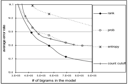
Figure 2 shows how the CER varies with the bigram numbers in the models. For comparison, we also include in Figure 2 the results using count cutoff pruning. We can see that CER decreases as we keep more and more bigrams in the model. A steeper curve indicates a better pruning criterion.
The main result to notice here is that the rank-based pruning achieves consistently the best performance among all of them over a wide range of CER values, producing models that are at 55-85% of the size of the probability-based pruned models with the same CER. An example of the detailed comparison results is shown in Table 1, where the CER is 13.8% and the value of cutoff is 1. The last column of Table 1 shows the relative model sizes with respect to the probability-based pruned model with the CER 13.8%.
Another interesting result is the good performance of count cutoff, which is almost overlapping with probability-based pruning at larger model sizes 2 . The entropy-based pruning unfortunately, achieved the worst performance.
13.6 13.7 13.8 13.9 14.0 14.1
3.E+05 4.E+05 5.E+05 6.E+05 7.E+05 8.E+05 9.E+05 # of bigrams in the model
av
er
age er
ro
r r
at
e
rank
prob
entropy
[image:4.612.321.533.244.318.2]count cutoff
[image:4.612.80.297.413.555.2]Figure 2: Comparison of pruning criteria
Table 1: LM size comparison at CER 13.8%
criterion # of bigram size (MB) % of prob
probability 774483 6.1 100.0%
cutoff (=1) 707088 5.6 91.8%
entropy 1167699 9.3 152.5%
rank 512339 4.1 67.2%
2 The result is consistent with that reported in (Goodman
and Gao, 2000), where an explanation was offered.
We assume that the superior performance of rank-based pruning lies in the fact that rank (acting as a LM evaluation measure) has better correlation with CER. Clarkson and Robinson (2001) estimated the correlation between LM evaluation measures and word error rate in a speech recognition system. The related part of their results to our study are shown in Table 2, where r is the Pearson product-moment correlation coefficient, rs is the
Spearman rank-order correlation coefficient, and T is the Kendall rank-order correlation coefficient.
Table 2: Correlation of LM evaluation measures
with word error rates (Clarkson and Robinson, 2001)
r rs T
Mean log rank 0.967 0.957 0.846 Perplexity 0.955 0.955 0.840 Mean entropy -0.799 -0.792 -0.602
Table 2 indicates that the mean log rank (i.e. related to the pruning criterion of rank we used) has the best correlation with word error rate, followed by the perplexity (i.e. related to the pruning criterion of probability we used) and the mean entropy (i.e. related to the pruning criterion of entropy we used), which support our test results. We can conclude that the LM evaluation measures which are better correlated with error rate lead to better pruning criteria.
5
Combining Two Criteria
We now investigate methods of combining pruning criteria described above. We begin by examining the overlap of the bigrams pruned by two different criteria to investigate which might usefully be combined. Then the thresholding pruning algorithm described in Figure 1 is modified so as to make use of two pruning criteria simultaneously. The problem here is how to find the optimal settings of the pruning threshold pair (each for one pruning criterion) for different model sizes. We show how an optimal function which defines the optimal settings of the threshold pairs is efficiently established using our techniques.
5.1 Overlap
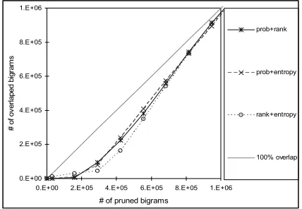
From the abovementioned three pruning criteria, we investigated the overlap of the bigrams pruned by a pair of criteria. There are three criteria pairs. The overlap results are shown in Figure 3.
[image:4.612.80.300.601.711.2]the model size decreases, but all criterion-pairs have overlaps much lower than 100%. In particular, we find that the average overlap between probability and entropy is approximately 71%, which is the biggest among the three pairs. The pruning method based on the criteria of rank and entropy has the smallest average overlap of 63.6%. The results suggest that we might be able to obtain improvements by combining these two criteria for bigram pruning since the information provided by these criteria is, in some sense, complementary.
0.E+00 2.E+05 4.E+05 6.E+05 8.E+05 1.E+06
0.E+00 2.E+05 4.E+05 6.E+05 8.E+05 1.E+06
# of pruned bigrams
# of
ov
er
la
ped bi
gr
am
s
prob+rank
prob+entropy
rank+entropy
[image:5.612.81.295.211.359.2]100% overlap
Figure 3: Overlap of selected bigrams between
criterion pairs
5.2 Pruning by two criteria
In order to prune a bigram model based on two criteria simultaneously, we modified the thresholding pruning algorithm described in Figure 1. Let lfi be the value of the performance loss
estimated by the loss function LFi, θi be the
threshold defined by the pruning criterion Ci. The
modified thresholding pruning algorithm can be described as follows:
1. Select a setting of threshold pair (θ1θ2)
2. Compute the values of performance loss lf1
and lf2 due to pruning each bigram
individually using the two pruning criteria C1 and C2, respectively.
3. Remove all bigrams with performance loss lf1 less than θ1, and lf2 less than θ2.
4. Re-compute backoff weights.
Figure 4: Modified thresholding algorithm for
bigram pruning
Now, the remaining problem is how to find the optimal settings of the pruning threshold pair for different model sizes. This seems to be a very tedious task since for each model size, a large number of settings (θ1θ2) have to be tried for finding
the optimal ones. Therefore, we convert the problem to the following one: How to find an optimal function θ2=f(θ1) by which the optimal threshold θ2
is defined for each threshold θ1. The function can be
learned by pilot experiments described below. Given two thresholds θ1 and θ2 of pruning criteria C1 and C2, we try a large number of values of θ1,θ2, and
build a large number of models pruned using the algorithm described in Figure 4. For each model size, we find an optimal setting of the threshold setting (θ1θ2) which results in a pruned model with
the lowest CER. Finally, all these optimal threshold settings serve as the sample data, from which the optimal function can be learned. We found that in pilot experiments, a relatively small set of sample settings is enough to generate the function which is close enough to the optimal one. This allows us to relatively quickly search through what would otherwise be an overwhelmingly large search space.
5.3 Results
We used the same training data described in Section 4 for bigram model training. We divided the test set described in Section 4 into two non-overlapped subsets. We performed testing on one subset containing 80% of the test set. We performed optimal function learning using the remaining 20% of the test set (referred to as held-out data below).
Take the combination of rank and entropy as an example. An uncompressed bigram model was first built using all training data. We then built a very large number of pruned bigram models using different threshold setting (θrank θentropy), where the
values θrank, θentropy∈ [3E-12, 3E-6]. By evaluating
[image:5.612.317.532.554.735.2]pruned models on the held-out data, optimal settings can be found. Some sample settings are shown in Table 3.
Table 3: Sample optimal parameter settings for
combination of criteria based on rank and entropy # bigrams θrank θentropy
137987 8.00E-07 8.00E-09
196809 3.00E-07 8.00E-09
200294 3.00E-07 5.00E-09
274434 3.00E-07 5.00E-10
304619 8.00E-08 8.00E-09
394300 5.00E-08 3.00E-10
443695 3.00E-08 3.00E-10
570907 8.00E-09 3.00E-09
669051 5.00E-09 5.00E-10
892214 5.00E-12 3.00E-10
892257 3.00E-12 3.00E-10
In experiments, we found that a linear regression model of Equation (6) is powerful enough to learn a function which is close enough to the optimal one.
2 1 log( ) )
log(θentropy =α × θrank +α (6)
Here α1 and α2 are coefficients estimated from the sample settings. Optimal functions of the other two threshold-pair settings (θ rankθprobability) and (θ probabilityθentropy) are obtained similarly. They are
shown in Table 4.
Table 4. Optimal functions
5
.
6
)
log(
3
.
0
)
log(
θ
entropy=
×
θ
rank+
2 . 6 )
log(θprobability = , for any θrank
5 . 3 ) log( 7 . 0 )
log(θentropy = × θprobability +
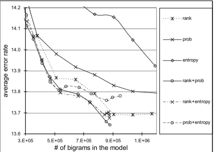
[image:6.612.78.299.73.107.2]In Figure 5, we present the results using models pruned with all three threshold-pairs defined by the functions in Table 4. As we expected, in all three cases, using a combination of two pruning criteria achieves consistently better performance than using either of the criteria separately. In particular, using the combination of rank and entropy, we obtained the best models over a wide large of CER values. It corresponds to a significant size reduction of 15-54% over the probability-based LM pruning at the same CER. An example of the detailed comparison results is shown in Table 5.
Table 5: LM size comparison at CER 13.8%
Criterion # of bigram size (MB) % of prob
Prob 1036627 8.2 100.0%
Entropy 1291000 10.2 124.4%
Rank 643411 5.1 62.2%
Prob + entropy 542124 4.28 52.2%
Prob + rank 579115 4.57 55.7%
rank + entropy 538252 4.25 51.9%
There are two reasons for the superior performance of the combination of rank and entropy. First, the rank-based pruning achieves very good performance as described in Section 4. Second, as shown in Section 5.1, there is a relatively small overlap between the bigrams chosen by these two pruning criteria, thus big improvement can be achieved through the combination.
6
Conclusion
The research on backoff n-gram pruning has been focused on the development of the pruning criterion, which is used to estimate the performance loss of the pruned model.
This paper explores several pruning criteria for backoff n-gram model size reduction. Besides the widely used probability, two new pruning criteria have been developed based on rank and entropy. We have performed an empirical comparison of these pruning criteria. We also presented a thresholding algorithm for model pruning, in which two pruning criteria can be used simultaneously. Finally, we described our techniques of finding the optimal setting of the threshold pair given a specific model size.
We have shown several interesting results. They include the confirmation of the estimation that the measures which are better correlated with CER for LM evaluation leads to better pruning criteria. Our experiments show that rank, which has the best correlation with CER, achieves the best performance when there is only one criterion used in bigram model pruning. We then show empirically that the overlap of the bigrams pruned by different criteria is relatively low. This indicates that we might obtain improvements through a combination of two criteria for bigram pruning since the information provided by these criteria is complementary. This hypothesis is confirmed by our experiments. Results show that using two pruning criteria simultaneously achieves
13.6 13.7 13.8 13.9 14.0 14.1 14.2
3.E+05 5.E+05 7.E+05 9.E+05 1.E+06
# of bigrams in the model
aver
age e
rror r
a
te
rank
prob
entropy
rank+prob
rank+entropy
[image:6.612.84.293.527.675.2]prob+entropy
Figure 5: Comparison of combined pruning
better bigram models than using either of the criteria separately. In particular, the combination of rank and entropy achieves the smallest bigram models at the same CER.
For our future work, more experiments will be performed on other language models such as word-based bigram and trigram for Chinese and English. More pruning criteria and their combinations will be investigated as well.
Acknowledgements
The authors wish to thank Ashley Chang, Joshua Goodman, Chang-Ning Huang, Hang Li, Hisami Suzuki and Ming Zhou for suggestions and comments on a preliminary draft of this paper. Thanks also to three anonymous reviews for valuable and insightful comments.
References
Clarkson, P. and Robinson, T. (2001), Improved language modeling through better language model evaluation measures, Computer Speech and Language, 15:39-53, 2001.
Gao, J. and Lee K.F (2000). Distribution-based pruning of backoff language models, 38th Annual meetings of the Association for Computational Linguistics (ACL’00), HongKong, 2000.
Gao, J., Goodman, J., Li, M., and Lee, K. F. (2002). Toward a unified approach to statistical language modeling for Chinese. ACM Transactions on Asian Language Information Processing, Vol. 1,
No. 1, pp 3-33. Draft available from
http://www.research.microsoft.com/~jfgao Goodman, J. and Gao, J. (2000) Language model
size reduction by pruning and clustering, ICSLP-2000, International Conference on Spoken Language Processing, Beijing, October 16-20, 2000.
Jelinek, F. (1990). Self-organized language
modeling for speech recognition. In Readings in Speech Recognition, A. Waibel and K. F. Lee, eds., Morgan-Kaufmann, San Mateo, CA, pp. 450-506.
Katz, S. M., (1987). Estimation of probabilities from sparse data for other language component of a speech recognizer. IEEE transactions on Acoustics, Speech and Signal Processing, 35(3):400-401, 1987.
Rosenfeld, R. (1996). A maximum entropy approach to adaptive statistical language modeling. Computer, Speech and Language, vol. 10, pp. 187-- 228, 1996.
Seymore, K., and Rosenfeld, R. (1996). Scalable backoff language models. Proc. ICSLP, Vol. 1., pp.232-235, Philadelphia, 1996