Munich Personal RePEc Archive
On the predictability of economic
structural change by the
Poincaré-Bendixson theory
Stijepic, Denis
University of Hagen
8 August 2017
1
On the predictability of economic structural change by the Poincaré-Bendixson theory
Denis Stijepic*
University of Hagen
17th August 2017
Abstract. The three-sector framework (relating to agriculture, manufacturing, and services) is one of the major concepts for studying the long-run change of the economic structure. We discuss the system-theoretical classification of the structural change phenomenon and, in particular, the predictability of the structural change in the three-sector framework by the Poincaré-Bendixson theory. To do so, we compare the assumptions of the Poincaré-Bendixson theory to (a) the typical axioms of structural change modelling, (b) the empirical evidence on the geometrical properties of structural change trajectories, and (c) some methodological arguments referring to the laws of structural change. The results of this comparison support the assumption that the structural change phenomenon is representable by a dynamic system that is predictable by the Poincaré-Bendixson theory. Moreover, we discuss briefly the implications of this result for structural change modelling and prediction as well as topics for further research.
Keywords. Poincaré-Bendixson theory, application, economics, structural change, labor reallocation, sectors, dynamics in the plane, simplex, trajectory, topology.
JEL codes. C61, C65, O41
Short Biography. Denis Stijepic has obtained a doctoral degree in economics from the University of Hagen in 2011. Currently, he is a researcher at the University of Hagen, Department of Macroeconomics.
_________________________________
* Address: Lehrstuhl für Makroökonomik, Fernuniversität in Hagen, Universitätsstrasse 41, D-58084 Hagen,
2
1. Introduction
The Poincaré-Bendixson theory, predicting the qualitative properties of the limit dynamics of smooth dynamic systems in the plane, is one of the fundaments of the dynamic systems theory. We discuss whether economic structural change is predictable by the Poincaré-Bendixson theory. While there are different notions of economic structure, we focus on the three-sector framework where structural change is indicated by the long-run dynamics of labor reallocation across the sectors ‘agriculture’, ‘manufacturing’, and ‘services’. The three-sector framework is one of the main concepts for studying the long-run dynamics of the macroeconomic structure. The related structural change and, in particular, industrialization and tertiarization are regarded as major drivers of economic development and have been
analyzed in numerous studies over the last 200 years.1
The question whether the structural change in the three-sector framework can be represented by a dynamic system that is predictable by the Poincaré-Bendixson is the key to a system-theoretical characterization of the three-sector framework and its long-run dynamics.2 Such a characterization is interesting for two reasons among others.
First, a ‘proof’ of the applicability of the Poincaré-Bendixson theory in the three-sector framework would not only allow us to characterize the limit-dynamics of structural change (i.e. to state that structural change is either transitory or cyclical in the limit, as we will see) but could also open the door for the application of other topological concepts, which can be used to predict the transitional structural change dynamics among others, in (a system-theoretical approach to) structural change analysis (see Stijepic (2015,2016,2017a) for an exploitation of the topological properties of structural change paths in structural change analysis). Such a characterization of transitional dynamics and limit-dynamics is usable for (long-run) structural change predictions, as demonstrated by Stijepic (2015,2017a).
Second, system-theoretical structural change models seem to be good complements to the standard structural change models (cf. Footnote 1). The latter generate relatively specific quantitative predictions of structural change. Yet, they are ideological to a great extent, since
1 For an overview of the structural change literature, see, e.g., Schettkat and Yocarini (2006), Krüger (2008),
Silva and Teixeira (2008), Stijepic (2011, Chapter IV), and Herrendorf et al. (2014). Recent papers modelling structural change in the three-sector framework are, e.g., Kongsamut et al. (2001), Ngai and Pissarides (2007), Foellmi and Zweimüller (2008), Uy et al. (2013), and Stijepic (2015,2017a).
2 To our knowledge, the Poincaré-Bendixson theory has not been applied in a system-theoretical study of the
3
they rely on very specific assumptions,3 specific schools of thought (e.g. neoclassical,
Keynesian, evolutionary, endogenous growth theory, etc.), and knife-edge parameter restrictions (cf. Stijepic (2011) and Temple (2003)), all of which are difficult to prove empirically and, thus, restrict the generality of models and the reliability of structural change predictions. In contrast, a system-theoretical modelling approach allows us to develop relatively general models generating relatively reliable predictions. Yet, such predictions are rather qualitative and encompass a relatively wide range of scenarios.
Our analysis of the predictability of structural change by the Poincaré-Bendixson theory can be classified as a system-theoretical contribution to structural change modelling. We do not seek to develop a fully specified economic model based on relatively specific and ideological assumptions regarding individual behavior and market-functioning, but rather analyze whether the assumptions of the Poincaré-Bendixson theory are supported by (a) the mathematical implications of the standard structural change definition and other mathematical structural change modelling conventions, (b) the empirical evidence on the topological properties of structural change trajectories, and (c) the methodological arguments relating to the representation of economic laws by economic models. This analysis allows us to assess whether the dynamic system representing the laws of structural change is of the Bendixson type (and, thus, structural change can be predicted by the Poincaré-Bendixson theory).
Owing to the geometrical/topological nature of the Poincaré-Bendixson theory (and its proof) our analytical approach is rather geometrical and topological. In particular, we exploit the fact that the Poincaré-Bendixson theory is applicable to a trajectory family that covers simply a bounded and connected subset of the plane. Such a covering has straight-forward geometrical characteristics (among others the trajectories are non-(self-)intersecting), which can be used to study the applicability of the Poincaré-Bendixson theory in structural change modelling, as we demonstrate.
Our results are in favor of the predictability of structural change by the Poincaré-Bendixson theory. Yet, some very interesting questions for further research remain open, which are summarized in Section 9.
The rest of the paper is structured as follows. In Section 2, we formulate a meta-model of structural change representing the standard axioms and definitions of structural change
3 For example, Kongsamut et al. (2001) focus on a demand-side explanation of structural change, Ngai and
4
modelling. Section 3 recapitulates briefly the relevant (primarily topological) concepts for dynamic systems analysis. In Section 4, we summarize the empirical evidence regarding the topological properties of structural change paths. Section 5 discusses the methodological aspects of structural change modelling. Section 6 recapitulates the assumptions (and their geometrical interpretation) and the results of the Poincaré-Bendixson theory. Section 7 is devoted to the comparison of the Poincaré-Bendixson assumptions (Section 6) with the empirics (Section 4) and the axiomatics (Section 2) of structural change modelling by relying on the topological notions introduced in Section 3 and the methodological arguments derived in Section 5. In Section 8, we discuss the interpretation of the (results of the) Poincaré-Bendixson theory in the context of structural change and the structural change predictions resulting from this interpretation. A summary of the results and a discussion of the topics for further research is provided in Section 9.
2. A mathematical meta-model of structural change (axiomatics of structural change) In this section, we recapitulate the mathematical meta-model of structural change that represents the modelling conventions of the structural change literature, as introduced by Stijepic (2015,2016,2017a). This model is fully specified by Definition 1 and Axioms 1-3. While Definition 1 relates model variables to the measures (in particular, employment shares) that are used to describe structural change in reality, Axioms 1-3 represent all the standard structural change modelling assumptions that cannot be proved by empirical evidence. Like all other empirical sciences, economics cannot work without relying on empirically improvable assumptions.
While there are different mathematical notational conventions, we choose the following
notation for reasons of simplicity: small letters (e.g. x), bold small letters (e.g. x), and capital
letters (e.g. X) denote scalars, vectors/points, and sets, respectively. A dot indicates a
derivative with respect to time (e.g. ẋ is the derivative of x with respect to time).
Definition 1. The sectors 1, 2, and 3 represent the primary (or agricultural) sector, the
secondary (or manufacturing) sector, and the tertiary (or services sector), respectively. y1c(t),
y2c(t), and y3c(t) denote the employment in sector 1, 2, and 3 at time t∈D⊆R in country c∈C,
respectively, where R is the set of real numbers. yc(t) is the aggregate employment at time t in
country c. xic(t) ∶= yic(t)/yc(t) is the employment share of sector i at time t in country c. The
5
country c. The term ‘structural change (over the period [a,b]) in country c’ refers to the
long-run dynamics of the labor allocation xc(t) (over the period [a,b]). The time point t = 0
represents the initial time point, and xc(0) ≡ (x1c(0), x2c(0), x3c(0)) stands for the initial labor
allocation in country c. If the initial labor allocation is given, we denote it by xc0≡ (x1c0, x2c0,
x3c0).
Consider the three-dimensional real space (R3) and the Cartesian coordinate system (x1, x2,
x3). We define the following set of points in it
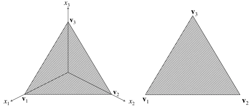
(1) S∶={x≡(x1, x2, x3)∈R3: x1+x2+x3=1 ∧∀i∈{1,2,3} 0 ≤ xi≤ 1}
It is well known that (a) S is a two-dimensional standard simplex (henceforth, 2-simplex), (b) the 2-simplex is a triangle, and (c) the Cartesian coordinates of its vertices are
(2) (1,0,0)=∶v1 (0,1,0)=∶v2 (0,0,1)=∶v3
[image:6.595.90.503.440.622.2]For an illustration, see Figure 1. Henceforth, we omit the coordinate axes, as depicted in the right panel of Figure 1.
Figure 1. The 2-simplex in the Cartesian coordinate system (x1,x2,x3) with and without
coordinate axes.
Axiom 1. (Cf. (1) and Definition 1.) The labor allocation function xc(t): D×C→S⊂R3 maps
time t∈D⊇[0,∞) and the country index c∈C to the 2-simplex S (which is located in the
coordinate system (x1, x2, x3)).
x3
v3
v2
v1 x
2
x1
v3
6
In particular, for a given country index c∈C, the function xc(t) assigns a point (x1, x2, x3) on
the 2-simplex S to each time point t∈D. Definition 1, Axiom 1, and (1) imply that the sectoral
employment shares satisfy the following conditions (3) ∀t ∀c ∀i∈{1,2,3} 0 ≤ xic(t) ≤ 1
(4) ∀t∀cx1c(t)+x2c(t)+x3c(t)=1
and ∀t ∀c yc(t) = y1c(t)+y2c(t)+y3c(t). These conditions are reasonable (e.g. the employment
shares cannot be negative) and represent standard assumptions in structural change modelling (see Stijepic (2015,2016,2017a) for a discussion).
Axiom 2.∀t∈D ∀c∈C, xc(t) is continuous in t.
Axiom 3.∀t∈D ∀c∈C, xc(t) is differentiable with respect to t.
The assumption of continuous and differentiable functional forms is not only standard in structural change modelling but also in major parts of growth theory, development theory, and theories of long-run dynamics, in general. For example, the models presented by Kongsamut et al. (2001), Ngai and Pissarides (2007), Acemoglu and Guerrieri (2008), Foellmi and Zweimüller (2008), and Boppart (2014) are typical examples of multi-sector models satisfying Axioms 2 and 3 (cf. Stijepic (2015,2016,2017a)).
Among others, we use the model specified in this section to compare the empirical evidence on structural change to the assumptions of the Poincaré-Bendixson theory. To do so, we have to introduce some concepts for describing the dynamics of the model of this section. We turn now to this topic.
3. Topological concepts for describing structural change
In this section, we recapitulate some topological concepts for analyzing structural change, as discussed by Stijepic (2015,2016,2017a).
Axiom 1 and Definition 1 imply that we can study the structural change in country c by
studying the properties of the function xc(t). In our paper, we choose a topological approach
7
Definition 2. The (image of the) structural trajectory (Tc) that depicts the structural change
(cf. Definition 1) in country c∈C over the time interval G⊆D is defined as follows:
(5) Tc(G)∶={xc(t)∈S: t∈G}.
Geometrically speaking, the economy c moves along Tc(G)⊂S over the time period G. Thus,
S is the domain of Tc(G).
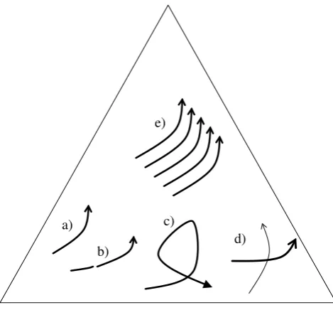
Trajectories can be characterized by using the (topological) concepts of continuity, self-intersection, and in the case of two or more trajectories (where each trajectory represents the structural change in a different country), intersection. The intuitive/geometrical notion of
continuity, self-intersection, and intersection is more or less obvious. For a continuous and
non-self-intersecting trajectory, see Figure 2a; in contrast, Figures 2b and 2c depict examples
[image:8.595.179.414.401.619.2]of non-continuous and self-intersecting trajectories, respectively. Figure 2d depicts two intersecting trajectories, whereas Figure 2e depicts non-intersecting trajectories.
Figure 2. Examples of (non-)continuous, (non-)self-intersecting, and (non-)intersecting
trajectories on S.
In our paper, we apply the following formal definitions of continuity, non-self-intersection, and non-intersection (cf. Stijepic (2015,2016,2017a)).
Definition 3. The trajectory (5) is continuous on S (for a given c∈C) if the corresponding
function xc(t) is continuous (in t) on the interval G (for the given c). a)
b)
c)
8
Definition 4. The (continuous and non-closed) trajectory (5) is non-self-intersecting (for a
given c∈C) if ∄(t1,t2,t3)∈G3: t1<t2<t3∧xc(t1)=xc(t3)≠xc(t2).
Definition 5. Two trajectories (Tp(A) and Tq(B), where p,q∈C and A,B⊆D) intersect if Tp(A)∩
Tq(B) ≠∅. Otherwise, if Tp(A)∩Tq(B) = ∅, the trajectories Tp(A) and Tq(B) do not intersect.
The Poincaré-Bendixson theory deals with the limit dynamics. The term ‘limit dynamics’
refers to the dynamics for t→∞. The Poincaré-Bendixson theory relies on the concept of the
‘omega limit set’ for describing the limit dynamics.
Definition 6. (Stijepic (2017a)) Let the function xc(t) satisfy the Axioms 1-3. The point xc* is
an omega limit point of the trajectory Tc([0,∞)) (cf. (5)) if there exists a sequence of time
points tk (where k=0,1,2,…) that satisfies two conditions: (a) tk converges to infinity (i.e.
tk→∞ for k→∞), and (b) the corresponding sequence xc(tk) converges to xc* (i.e. xc(tk)→xc*
as tk→∞). The omega limit set O(Tc([0,∞))) of the trajectory Tc([0,∞)) is the union of all
omega limit points of the trajectory Tc([0,∞)).
For a discussion and explanation of the omega limit set, see, e.g., Andronov et al. (1987, p.353ff.), Walter (1998, p.322), and Hale (2009, p.46f.). The (type of the) limit dynamics of
an economy that moves along the trajectory image Tc is indicated by the omega limit set of
the trajectory Tc, as we will see in Section 8. Finally, we introduce two (non-topological)
concepts that help us to describe the empirical evidence discussed in Section 4.
Definition 7. The set M is the minimal convex subset of S covering the trajectory family B⊆C
(cf. Definition 2) if (a) M⊆S, (b) M is convex, (c) ⋃𝑐∈𝐵Tc([0,∞))⊆M, and (d) among all the
sets satisfying the criteria (a)-(c), M covers the smallest area of S.
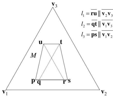
Definition 8. Let M be a (convex) subset of S. Let L1 be the set of all line-segments that (a)
connect two boundary points of M and (b) are parallel to the line-segment 𝐯������2𝐯3. Let l1 be the
line-segment that has the greatest length among all the line-segments belonging to the set L1
(cf. Figure 3). d1 is the length of l1. Analogously, let L2 (L3) be the set of all line-segments that
9
Let l2 (l3) be the line-segment that has the greatest length among all the line-segments
[image:10.595.182.415.161.367.2]belonging to the set L2 (L3). d2 (d3) is the length of l2 (l3).
Figure 3. An example illustrating l1, l2, and l3.
Definitions 7 and 8 allow us to measure the diameter of the minimal subset covering a family
of trajectories in the three relevant directions on S. In fact, the diameter vector (d1, d2, d3) is a
(crude) measure of the heterogeneity of a trajectory family on S. The greater the diameters d1
-d3, the greater the differences between the labor shares covered by the trajectories belonging
to a trajectory family.
4. Empirical regularities of structural change (empirics of structural change)
While several stylized facts (or empirical regularities) of structural change are known (see Stijepic (2015,2016,2017a) for an overview), we focus on Regularities 1-3, which will prove useful for assessing the applicability of the Poincaré-Bendixson theory later. For empirical evidence on Regularities 1 and 3 and theoretical explanations, see Stijepic (2015,2016, 2017a). Figure 4 presents evidence supporting Regularities 1-3.
Regularity 1. (Stijepic (2015,2016,2017a)) The long-run dynamics of labor allocation in the
three-sector framework can be represented by non-self-intersecting trajectories.
Regularity 2. The labor-allocation trajectories differ significantly across countries. The
minimal convex set M covering the trajectories representing the labor-allocation dynamics of
10
the OECD countries over the last 200 years is relatively large (cf. Definition 7). In
particular, the diameters d1, d2, and d3 of the set M are relatively large (cf. Definition 8).
Regularity 3. (Stijepic (2016)) The (long-run) labor allocation trajectories of different
[image:11.595.92.515.243.617.2]countries intersect.
Figure 4.Labor allocation trajectories of USA, France, Germany, Netherlands, UK, Japan,
China, and Russia.
Notes: Data source: Maddison (1995). The black dot represents the barycenter of the simplex. Abbreviations: C
– China, F – France, G – Germany, J – Japan, N – Netherlands, R – Russia, US – United States, UK – United
Kingdom. Data points (years in parentheses): USA (1820, 1870, 1913, 1950, 1992), France (1870, 1913, 1950,
1992), Germany (1870, 1913, 1950, 1992), Netherlands (1870, 1913, 1950, 1992), UK (1820, 1870, 1913, 1950,
1992), Japan (1913, 1950, 1992), China (1950, 1992), Russia (1950, 1992). v1
v3
v2 C US
J
G
UK F R
11
5. Some methodological aspects
5.1 Topological properties of models representing laws
Economic modelling and predicting, as modelling and predicting in other sciences, relies on the assumption that the concepts/variables being modelled obey some sort of laws that can be expressed by mathematical equations/relations and are valid for different states of the environment and across time to some extent (since otherwise modelling and predicting would be obsolete). In particular, it is preferable that a (structural change) model (cf. Footnote 1)
generates a family of curves (e.g., x(t,x0,p): G×S×P→S; cf. Definition 1) that represent
different initial states (x0) of the system and different parameter settings (p) of the model.
Given a connected state space (S), a connected parameter space (P), and an empirically
observed ‘typical’ trajectory that is representable by a generic model trajectory (x(t,x0,p):
G→S, x0∈S, p∈P), a model (representing laws) should be able to generate a new generic
trajectory for a marginal deviation of the initial state from the observed initial state x0∈S (and
for a marginal deviation of model parameters from the assumed/observed parameter setting
p∈P; cf., e.g., Andronov et al. (1987, p.374 and p.405)). In other words, the trajectory family
generated by a model representing (economic) laws should not only contain a generic trajectory that is sufficiently similar to an empirically observed ‘typical’ trajectory but should also cover completely a connected subset (H) of the state space (S) containing the generic
model trajectory that represents the typical empirical trajectory.4 Otherwise, the model would
not be empirically relevant since initial states, parameters, and observed states (i.e. the typical trajectory) are not measurable exactly and we must assume that the ‘real’ initial states, parameters, and trajectories deviate from their observed/measured values and from the
generic model trajectory representing them (cf. Andronov et al. (1987, p.374 and p.405)).5 As
we will see in Section 6.1, the extendibility of model predictions to a connected subset of the state (and parameter) space is a characteristic of (smooth) differential equation systems and, in particular, of the differential equation systems to which the Poincaré-Bendixson theory applies. For these reasons (among others) such systems are widespread in modelling of physical systems obeying physical laws.
4 The analogous is true for a parameter setting variation: the representative trajectory family should contain
trajectories for all values of a connected subset (Q) of the parameter space (P) containing the parameter setting of the representative trajectory, to ensure ‘coarseness’.
5 For example, a model that can explain the dynamics of country c if the initial agricultural share in country c is
12
This discussion has a major implication for the meta-model presented in Section 2, as discussed in Section 5.2.
5.2 Implications for the meta-model of Section 2
Empirical evidence implies that structural change seems to follow some ‘laws’ (or rules/regularities), which are quite persistent across countries and time (see Stijepic (2017a)
for a summary and literature references). Economic laws can be understood as ceteris paribus
laws (cf., e.g., Jackson and Smith (2005) and Reutlinger et al. (2015)). This is reflected by the fact that standard structural change models (cf. Footnote 1) are dependent on parameters (e.g. time-preference rate and technology parameters) that, in general, may vary across countries. A most obvious example of observable cross-country parameter variation are the technology differences between developed and underdeveloped economies. Moreover, as implied by Regularity 2, the structural trajectories of the OECD countries (covering the last 200 years)
differ significantly, such that we have to assume that the initial states xc0 (cf. Definition 1)
differ significantly across countries c (when choosing an initial time point within the last 200 years, which is a standard choice in structural change modelling). Thus, it makes sense to assume that the meta-model of Section 2 representing the dynamics of different countries (indexed by the index c and the index set C) represents different initial states and different parameter values of a structural change model. Then, the arguments elaborated in Section 5.1 imply that if the meta-model of Section 2 represents economic (structural change) laws and is of empirical relevance, we should assume that the trajectory family defined by Axioms 1-3 (and indexed by the set C) covers completely a connected subset H of the state space S, i.e. (6) ⋃𝑐∈𝐶Tc([0,∞))⊇H
where the index set C, the relevant state space H, and the trajectories Tc represent at least
some countries that have typical structural change patterns.
6. The Poincaré-Bendixson theory
13
6.1 The Poincaré-Bendixson assumptions and their topological interpretation
First, we recapitulate some elementary differential equation theory. Consider an autonomous differential equation system in the plane associated with the following initial value problem: (7) ẏ(t) = Φ(y(t)), y(0) = y0∈H⊆R2, Φ: H→R2, t∈D⊇[0,∞)
where Φ is a vector function, D an interval, and H an open and connected subset of R2. A solution of the initial value problem (7) on the interval D is a vector function y(t): D→H, satisfying y(0) = y0.
If the function Φ is sufficiently smooth, then there exist unique solutions of the initial value
problem (7) for all y0∈H (see, e.g., Walter (1998), p.108 and p.110f.). For example, if Φ is
analytical, continuous and continuously differentiable, or Lipschitz-continuous, then the
uniqueness of solutions of (7) is ensured (see, e.g., Stijepic (2015, p.84f.) for a list of (exact) conditions ensuring uniqueness of solutions and literature references). The Poincaré-Bendixson theory applies to the differential equation systems in the plane (of the type (7))
that are sufficiently smooth to ensure the uniqueness of their solutions(see, e.g., Andronov et
al. (1987, p.351ff.), Guckenheimer and Holmes (1990, p.43f.), Hale (2009, p.51ff.), and Teschl (2011, Chapter 7.3)). Henceforth, we name these systems ‘sufficiently smooth autonomous differential equation systems in the plane’ (abbreviated ‘SSADES’).
Given the set H of initial values, a SSADES generates a family (F) of trajectories/curves that have the following (topological) characteristics (cf. Walter (1998, p.10, p.36, and p.110f.), Hale (2009, p.18f. and p.38f.), and Stijepic (2015, p.84f.)).
Property 1. (Continuity.) Each trajectory belonging to the family F is continuous (cf.
Definition 3).
Property 2. (Non-self-intersection.) Each trajectory belonging to the family F is
non-self-intersecting (cf. Definition 4).
Property 3. (Non-intersection.) The trajectories belonging to the family F are
non-intersecting (cf. Definition 5).
14
that we reach the (regular) point q∈H, then q is either on the trajectory τ or on another
trajectory belonging to the trajectory family F.
Finally, note that the Poincaré-Bendixson theory applies only to bounded trajectories (cf. Section 6.2). Thus, we postulate the following property.
Property 5. (Boundedness.) The trajectory under consideration is bounded.
Overall, Properties 1-5 characterize SSADES to which the Poincaré-Bendixson theory applies. Thus, we will use these properties to discuss/test whether the structural change axioms/empirics are consistent with the assumptions of the Poincaré-Bendixson theory. Note that even non-autonomous differential equation systems can generate trajectory families that have the Properties 1-5 and that are predictable by the Poincaré-Bendixson theory. Thus, Properties 1-5 constitute rather a test of the applicability of the Poincaré-Bendixson theory (in structural change modelling) than a test of the autonomy of the differential equation system (describing the dynamics of structural change).
Note that the Poincaré-Bendixson theory is restricted to the dynamic systems or the subsets (H) of the state space that do not generate/contain an infinite number of fixed points (see, e.g., Andronov et al. (1987, p.351f.) and Hale (2009, p.55)). Since we cannot evaluate economically or empirically this requirement/assumption, we assume, henceforth, that it is satisfied (i.e. the number of fixed points is finite). Giving an intuitive economic meaning to this assumption is an interesting topic for further research. Moreover, there are generalizations of the Poincaré-Bendixson theory (e.g. Solntzev (1945)) allowing for infinitely many fixed points (see, e.g., Ciesielski (2012, p.2117f.) and Nikolaev and Zhuzhoma (1999, p.37)). Further research could use these generalizations as a starting point.
6.2 The Poincaré-Bendixson results
Let Y([0,∞)):={y(t)∈H: t∈[0,∞)} denote (the image of) a bounded (half-)trajectory on an open
and connected subset (H) of the plane R2, where the function y(t): D→H represents the
solution of a SSADES in the plane (for some given initial value y0∈H) and D⊇[0,∞) is an
(open) interval (cf. Section 6.1).6 The Poincaré-Bendixson theory states that then, one of the
following statements is true (cf. Definition 6, Andronov et al. (1987, p.362f.), Guckenheimer
6 Recall that we assume here that the SSADES is such that it does not generate an infinite number of fixed
15
and Holmes (1990, p.45), Hale (2009, p.55 and, in particular, Theorem 1.3) and Teschl (2011, Chapter 7.3 and, in particular, Theorem 7.16)):
(i) O(Y([0,∞))) is a fixed point (critical point).
(ii) O(Y([0,∞))) is (the image of) a Jordan curve.
(iii) O(Y([0,∞))) is (the image of) a homoclinic orbit (including its fixed point).
(iv) O(Y([0,∞))) is a union of at least two fixed points and the (images of the) trajectories
connecting them (‘heteroclinic union’).
Note that (a) the term ‘heteroclinic union’ is not common in the literature and we use it here only as an abbreviation and (b) a ‘heteroclinic union’ must contain heteroclinic trajectories and can contain homoclinic trajectories.
We interpret and discuss the cases (i)-(iv) in the context of structural change in Section 8.
7. Comparison of the Poincaré-Bendixson assumptions to the axiomatics and empirics
of structural change analysis via topology and methodology
Now, we can turn to the question of the applicability of the Poincaré-Bendixson theory in structural change modelling. Due to the spadework of the previous sections, this comparison is relatively straight-forward.
As discussed in Section 6.1, the Poincaré-Bendixson theory applies to a bounded trajectory generated by a dynamic system that generates a family of trajectories that are continuous, non-(self-)intersecting and simply cover a subset of the plane, i.e. the Poincaré-Bendixson theory applies to a family of trajectories characterized by the Properties 1-5. Our axiomatic model formulated in Section 2, the empirical evidence presented in Section 4, and the methodological arguments discussed in Section 5.2 are consistent with the assumption of such a system, as explained in the following.
Obviously, Axioms 1-3 support Property 1. Property 2 is clearly supported by the empirical
evidence (cf. Regularity 1).
Property 3 and Regularity 3 seem to contradict each other at first sight. However, Property 3 and Regularity 3 are not necessarily inconsistent. We have shown in Section 5.2 that (a) the structural change models represent ceteris paribus laws such that their predictions depend on
parameters, which differ across countries, and (b) the countries differ by initial states xc0
given the standard horizon of structural change analysis (of ca. 200 years). If the parameters of a SSADES (cf. Section 6.1) differ across countries and countries are characterized by
different initial states xc0, intersections of the trajectories representing different countries may
16
as evidence against Property 3, and the study of the causes of the observable intersections (i.e. the analysis of the question whether Regularity 3 represents cross-country differences in parameters of the dynamic system generating the structural dynamics) is an interesting and very extensive topic for further research that could help to establish the validity of Property 3 (and the Poincaré-Bendixson theory) in structural change modelling. Moreover, there are theories/models (e.g. the Kongsamut et al. (2001) model and the Ngai and Pissarides (2007)
model) that generate equilibriums7 that represent the long-run economic dynamics and are
characterized by non-intersecting labor allocation trajectories (see Stijepic (2016)); these models can be regarded as ‘theoretical’ arguments for modelling (long-run) structural change in a framework of non-intersecting trajectories (cf. Property 3).
The methodological arguments presented in Section 5.2 state that a structural change model should generate a family of trajectories that cover completely a bounded subset (H) of the state space. If we assume that a family (F) of trajectories satisfies this requirement and is characterized by Properties 1-3 (as discussed above), then obviously, this family (F) is characterized by Property 4 as well. In particular, if a family of trajectories is continuous (cf. Property 1), non-self-intersecting (cf. Property 2), non-intersecting (cf. Property 3), and covers completely the domain H (according to the arguments of Section 5.2), then obviously, this family covers simply the domain H (cf. Property 4).
Finally, note that Property 5 is consistent with the structural change meta-model presented in Section 2, since structural change is defined on the bounded domain S (cf. Axiom 1 and Figure 1).
8. On the interpretation/application of the Poincaré-Bendixson theory in the context of
structural change
Now, assume that we impose additional restrictions (cf. Sections 4-7) on the structural change meta-model of Section 2 such that it becomes predictable by the Poincaré-Bendixson
theory. According to Axiom 1, the structural change in the country c∈C is given by the
function xc(t): [0,∞)→S, and the Poincaré-Bendixson theory predicts that the omega limit-set
of this function is characterized by one and only one of the following scenarios (cf. Section 6.2 and Definition 2).
(i) O(Tc([0,∞))) is a fixed point (critical point).
(ii) O(Tc([0,∞))) is (the image of) a Jordan curve.
7 Kongsamut et al. (2001) (Ngai and Pissarides (2007)) name the long-run equilibrium arising in their model
17
(iii) O(Tc([0,∞))) is (the image of) a homoclinic orbit (including its fixed point).
(iv) O(Tc([0,∞))) is a union of at least two fixed points and (the images of) the trajectories
connecting them (‘heteroclinic union’). We can interpret the scenarios (i)-(iv) as follows.
In case (i), the labor allocation in economy c converges along the trajectory image Tc to a
fixed point (xc*) for t→∞, i.e. O(Tc([0,∞)))={xc*}. Thus, structural change is transitory, i.e. it
comes to a halt in the limit.
Case (ii) is known from the Poincaré-Bendixson theorem (see, e.g., Miller and Michel (2007,
p.290ff.) or Hale (2009, p.51ff.)). O(Tc([0,∞))) is the image of a Jordan curve in case (ii).
Thus, Tc represents either (a) a closed trajectory (i.e. a Jordan curve) or (b) a non-closed
trajectory converging to a closed trajectory (i.e. the labor allocation in economy c converges to a limit cycle).
In cases (iii) and (iv), for t→∞, the labor allocation in economy c converges along the
trajectory image Tc to (all) the points of the homoclinic orbit or to (all) the points of the
‘heteroclinic union’, per definition of the term omega limit set (cf. Definition 6). Therefore, structural change is cyclical in the limit (cf. Figures 5 and 6, which are based on Andronov et al. (1987, p.362)).
Overall, the Poincaré-Bendixson theory allows us to reduce the number of potential structural change limit-scenarios to only two qualitative scenarios stating that structural change is either transitory or cyclical in the limit. The standard structural change literature (cf. Footnote 1) implies, in general, that structural change is transitory. Thus, our meta-model (i.e. the Poincaré-Bendixson theory) generalizes this result. The cyclicality of structural change is interesting since it implies, e.g., unemployment (associated with reallocation of labor across sectors) and other fluctuations caused by structural change (e.g. productivity fluctuations). Moreover, cyclical structural change behavior seems to be ‘inefficient’ from the macroeconomic perspective since it causes structural change costs (see Stijepic (2016,2017b)). However, the empirical evidence shows that there are some short-run fluctuations with respect to structural change and, in particular, the structural change trajectories seem to have loops (on S) covering rather short periods of time (cf. Stijepic (2016,2017a)). Thus, cyclicality of structural change is not an irrelevant concept from the empirical point of view.
18
[image:19.595.178.412.306.494.2]empirical information on structural change. For example, Stijepic (2015) demonstrates by using an axiomatic/geometric approach that if the continuity and non-self-intersection properties (i.e. Properties 1 and 2) are combined with the fact that underdeveloped (advanced) economies are dominated by agriculture (services), the number of future structural change scenarios (in developed and emerging countries) can be reduced significantly, thus, yielding interesting meta-model predictions of structural change. Further research could focus on combining Properties 1-5 with other empirical information on the geometrical properties of structural change trajectories and deriving predictions of structural change based on them (see Stijepic (2017a) for an overview of such empirically observable geometrical properties of structural change trajectories).
Figure 5. Example: O(Tc([0,∞))) is the image of a homoclinic orbit.
Figure 6. Example: O(Tc([0,∞))) is a ‘heteroclinic union’.
.
.
: ))) , 0 ([ (Tc ∞O ∪ c T )) , 0 ([ ∞ c T
.
.
)) , 0 ([ ∞ c T.
: ))) , 0 ([(Tc ∞
O ∪
c
[image:19.595.187.408.558.732.2]19
9. Concluding remarks
The Poincaré-Bendixson theory is a prototype system theory. It is applicable to a wide range of real world physical systems. While economic systems (which are often describable by ceteris paribus laws and non-autonomous differential equations) are quite different in comparison to physical systems, the long-run structural change in the three-sector framework seems to be quite similar to physical phenomena, since it obeys economic laws that are quite robust across countries and time. Therefore, we devoted this paper to the analysis of the question whether structural change behaves like one of the typical physical phenomena that can be described by the Poincaré-Bendixson theory.
We have chosen a rather innovative way of doing so. While it is possible to justify the applicability of the Poincaré-Bendixson theory in economics on the basis of theoretical assumptions (see, e.g., Coles and Wright (1998)), we have tried to rely on (a) the mathematical implications of standard structural change definitions and mathematical structural change modelling conventions, (b) empirical evidence, and (c) methodological arguments for establishing the validity of the Poincaré-Bendixson theory in structural change modelling aiming at a system-theoretical classification of the structural change phenomenon that is independent of specific economic assumption sets, schools of thought, and economic ideologies in general (cf. Section 1).
As noted in Section 7, it can be shown that some standard structural change models generate dynamic equilibriums that are consistent with (some of) the Poincaré-Bendixson assumptions (cf. Stijepic (2016)). However, neither does the application of the Poincaré-Bendixson theory in these models makes sense (since the assumptions of these models are sufficiently specific to solve the differential equation systems generated by them), nor generate these models the wide range of potential limit-scenarios (cf. Section 8) predicted by the Poincaré-Bendixson theory. Moreover, as discussed in Section 1, standard structural change models are characterized by many rather ‘ideological’ assumptions, such that their support of the applicability of the Poincaré-Bendixson theory in structural change modelling may be regarded as not very robust and, thus, our system-theoretical complement of these models seems to make sense.
20
economic development from the system-theoretical perspective and, thus, elaborate relatively robust (cf. Section 1) predictions of limit-structural change dynamics on the basis of the Poincaré-Bendixson theory and (b) the fact that structural change is representable by simple coverings implies in conjunction with other (empirical) structural change facts some
predictions/statements regarding the nature of transitional structural change dynamics, as
demonstrated by Stijepic (2015) (cf. Stijepic (2017a)). Further research could deal with the
continuation of the latter approach for elaborating further aspects of transitional structural
change dynamics.
Moreover, we have elaborated two relatively interesting topics for further research: (1.) the study of the case with infinitely many fixed points mentioned in Section 6.1 and (2.) the interpretation of the empirical evidence on the intersections of countries’ structural change trajectories and, in particular, the question whether these intersections can be explained by cross-country parameter variation (cf. Section 7).
10. References
Acemoglu, D., Guerrieri, V., 2008. Capital deepening and non-balanced economic growth. Journal of Political Economy 116 (3), 467–498.
Andronov, A.A., Vitt, A.A., Khaikin, S.E., 1987. Theory of oscillators. Dover Publications, Mineola, New York.
Boppart, T., 2014. Structural change and the Kaldor facts in a growth model with relative price effects and non-Gorman preferences. Econometrica 82 (6), 2167–2196.
Ciesielski, K., 2012. The Poincaré–Bendixson theorem: from Poincaré to the XXIst century. Central European Journal of Mathematics 10 (6), 2110–2128.
Coles, M.G., Wright, R., 1998. A dynamic equilibrium model of search, bargaining, and money. Journal of Economic Theory 78 (1), 32–54.
Foellmi, R., Zweimüller, J., 2008. Structural change, Engel’s consumption cycles and Kaldor’s facts of economic growth. Journal of Monetary Economics 55 (7), 1317–1328.
Guckenheimer, J., Holmes, P., 1990. Nonlinear oscillations, dynamical systems, and bifurications of vector fields. Springer, New York.
21
Jackson, Frank, and Smith, Michael, eds., 2005. The Oxford handbook of contemporary philosophy. Oxford University Press, New York.
Kongsamut, P., Rebelo, S., Xie, D., 2001. Beyond balanced growth. Review of Economic Studies 68 (4), 869–882.
Krüger, J.J., 2008. Productivity and structural change: a review of the literature. Journal of Economic Surveys 22 (2), 330–363.
Maddison, A., 1995. Monitoring the world economy 1820–1992. OECD Development Centre, Paris.
Miller, R.K., Michel, A.N., 2007. Ordinary differential equations. Dover Publications, Mineola, New York.
Ngai, R.L., Pissarides, C.A., 2007. Structural change in a multisector model of growth. American Economic Review 97 (1), 429–443.
Nikolaev, I., Zhuzhoma, E., 1999. Flows on 2-dimensional manifolds: an overview. Springer, Berlin.
Reutlinger, A., Schurz, G., Hüttemann, A., 2015. Ceteris paribus laws. The Stanford encyclopedia of philosophy (Fall 2015 Edition), Edward N. Zalta (ed.), URL: http://plato.stanford.edu/archives/fall2015/entries/ceteris-paribus/.
Schettkat, R., Yocarini, L., 2006. The shift to services employment: a review of the literature. Structural Change and Economic Dynamics 17 (2), 127–147.
Silva, E.G., Teixeira, A.A.C., 2008. Surveying structural change: seminal contributions and a bibliometric account. Structural Change and Economic Dynamics 19 (4), 273–300.
Solntzev, G., 1945. On the asymptotic behaviour of integral curves of a system of differential equations. Bulletin de l’Académie des Sciences de l’URSS, Série Mathématique 9 (3), 233– 240.
Stijepic, D., 2011. Structural change and economic growth: analysis within the partially balanced growth-framework. Südwestdeutscher Verlag für Hochschulschriften, Saarbrücken. An older version is available online: http://deposit.fernuni-hagen.de/2763/.
Stijepic, D., 2015. A geometrical approach to structural change modelling. Structural Change and Economic Dynamics 33, 71–85.
Stijepic, D., 2016. A topological approach to structural change analysis and an application to long-run labor allocation dynamics. MPRA Working Paper No. 74568.
22
Stijepic, D., 2017b. On development paths minimizing the structural change costs in the three-sector framework and an application to structural policy. Available at SSRN: https://ssrn.com/abstract=2919806
Temple, J., 2003. The long-run implications of growth theories. Journal of Economic Surveys 17 (3), 497–510.
Teschl, G., 2012. Ordinary differential equations and dynamical systems. American Mathematical Society, Providence, Rhode Island.
Uy, T., Yi, K.-M., Zhang, J., 2013. Structural change in an open economy. Journal of Monetary Economics 60 (6), 667–682.
23
Appendix
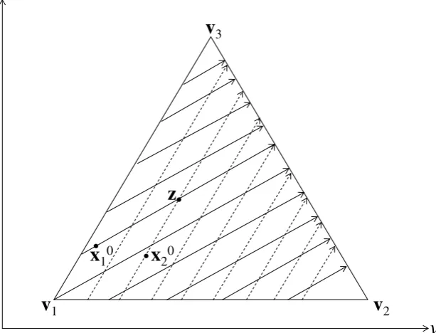
As discussed in Section 6.1, SSADES are characterized by non-(self-)intersecting trajectory families. In this appendix, we show that such a non-(self-)intersecting trajectory family can give rise to intersections of trajectories representing different countries if the parameter setting differs across countries.
Let (u,v) be a coordinate system that is parallel to S, such that all points on S can be identified
by their coordinates (u,v). Assume, moreover, a family of lines representing the images of
linear non-(self-)intersecting trajectories covering (a subset of) S and indicating a movement
away from vertex v1. Let this family of lines be given by the family of functions u = fb(a,v) =
a + bv, where fb(a,v): R2→R for a given b∈R. Assume that country 1 is characterized by b =
1/3 and country 2 is characterized by b = 2/3. Figure A1 illustrates the family of functions
fb(a,v), where the parameter setting b = 1/3 (b = 2/3) is represented by solid lines/arrows
(dashed lines/arrows) and only a subset of the line-segments that intersect with S is depicted.
Moreover, assume that the initial states xc0 of the countries are not identical (i.e. x10 ≠ x20)
and, thus, at t = 0, the countries are not located at the same place on S. As we can see in
Figure A1, the images of the trajectories of countries 1 and 2 intersect (at the point z),
[image:24.595.148.455.523.757.2]although each of the countries is modelled by a system of non-(self-)intersecting trajectories and the countries differ only by the parameter b.
Figure A1. An example of trajectory intersection arising from cross-country differences
regarding parameters and initial states.