Cellular and Dendritic Growth in Constrained Solidification
Yasunori Miyata
Nagaoka University of Technology, Department of Mechanical Engineering, Nagaoka 940-2188, Japan
A theoretical model is developed to predict the characteristics of a needle (cellular or dendrite) interface during the controlled and arrayed solidification of binary alloys. Both heat and mass transport fields near a growing needle front have been considered. The effect of solute, diffused from nearby dendrites, on dimensions of needle is also taken into account. Minimum undercooling criterion of tip of interface has been developed to select a solution to determine the dimensions, satisfying the local equilibrium conditions at the interface. Solutions are classified into two categories; one is responsible to the cellular growth and the other to the dendrite growth. Good correlations are obtained between theory and experiments. [doi:10.2320/matertrans.MB200701]
(Received March 1, 2007; Accepted April 23, 2007; Published July 11, 2007)
Keywords: dendrite, morphology, solidification, modeling, theory, primary-arm spacing, tip radius of curvature, undercooling, supercooling
1. Introduction
The importance of directional solidification studies has been well recognized since the early systematic scientific investigations carried out by Chalmers and co-workers1)to
understand the solidification characteristics of alloys. A majority of alloys grow under conditions which give rise to dendritic interface. For this reason, considerable theoretical and experimental attempts have been made to understand the characteristics of dendritic growth carried out under con-trolled solidification conditions. Unfortunately, no satisfac-tory treatment is available as yet which can quantitatively explain all the available experimental data and which correctly incorporate all the physics of the problem. It is the purpose of this paper to present a detailed theoretical model of cellular and dendritic growth under controlled solidification condition.
An approximate model of dendritic interface growth under controlled solidification conditions was given by Bower et al.2) They predicted that the undercooling, T
tip, at the
dendritic tip is given by the expression
Ttip¼ GLD
V
whereGL is the temperature gradient in liquid,Dthe solute diffusion coefficient in liquid, andV the growth rate. Such a formulation is valid only under large temperature gradient and low velocity values. Their treatment does not consider the variation of dendrite tip radius or sidewise diffusion near dendrite tip region.
The three-dimensional solute diffusion problem was treated by Burden and Hunt,3,4) and their results provided
an excellent qualitative understanding of the variation of tip temperature as a function ofGLandV. They assumed that, for a given temperature gradient, tip undercooling passes through a minimum as velocity increased.
Trivedi5) developed a formulation under the condition, which ensures that the dendrite tip is stable so that it can grow in steady-state fashion. Kurz and Fisher6)proposed another approach, where the radius of curvature of a dendrite tip was assumed to be proportional to the wavelength of perturbation in a planar interface. Their prediction provides a close
quantitative understanding of the radius of curvature of the dendrite tip as a function ofGLandV. The approach given by Kurz and Fisher suggests an essential importance of the diffusion from nearby dendrites to the tip.
A characteristic feature of constrained growth is the cellular morphology in low growth rate. Lu and Hunt7)have
analyzed numerically the feature of constrained growth and predicted dimensions of cellular and/or dendritic interface. They have pointed out the importance of boundary conditions in the interdendritic region in their simulation.
Theoretical models usually adopt a parabolic shape for the interface near the tip of dendrite. Bisang and Bilgram8)have observed the shape of Xenon dendrite tip and found that the tip shape of dendrite is very close to parabolic but necessarily perfectly parabolic. Phase field model.9,10)of dendrite growth
gives solutions stable when the crystalline anisotropy is introduced in the theory. The crystalline anisotropy11,12)will
be responsible to the deviation of interfacial shape near the tip from the parabolic one.
The purpose of this paper is to develop a consistent theory of cellular and/or dendrite growth which takes into account the heat flow and the solute one around the interface front, and which correctly predicts the limiting behavior of a planar interface at appropriate values of temperature gradient, growth rate, and solute composition. The effect of solute diffusion from nearby dendrites is incorporated in the theory, describing the solute distribution by the addition of solutions of diffusion equation for nearby dendrites. For the interface shape near tip of a dendrite, small deviation from parabolic shape is allowed in the theory. A condition, which will be closely related to the cellular growth, is imposed on the solute distribution in the interdendritic region. A solution is selected which gives the locally minimum undercooling at a tip of interface.
The temperature, composition, and dimensions(the tip radius of curvature and primary arm spacing) of the cellular and the dendrite tip will be predicted and compared with available experimental data.
2. General Description of Arrayed Cell/Dendrite
Consider a dendrite which is growing in the Z direction at Special Issue on Solidification Science and Processing for Advanced Materials
constant velocity, V, which is the direction of the dendrite axis of symmetry. Furthermore, we divide all coordinates by the tip radius of curvature of the dendrite, , to obtain a dimensionless coordinate system. Besides Cartesian coordi-nate, we shall also use dimensionless parabolic coordinates,
; and’, in which the dendritic interface will be represented by
2¼1þaa2 ðits tip coordinate ðx;y;zÞ ¼ ð0;0;0:5ÞÞ; ð1Þ
whereaais a parameter which represents the deviation from the parabolic shape. The dimensionless parabolic coordinates are related to the dimensionless Cartesian coordinates x;y
andzas
¼xycos’; ¼xysin’; z¼ ð22Þ=2 ð2Þ
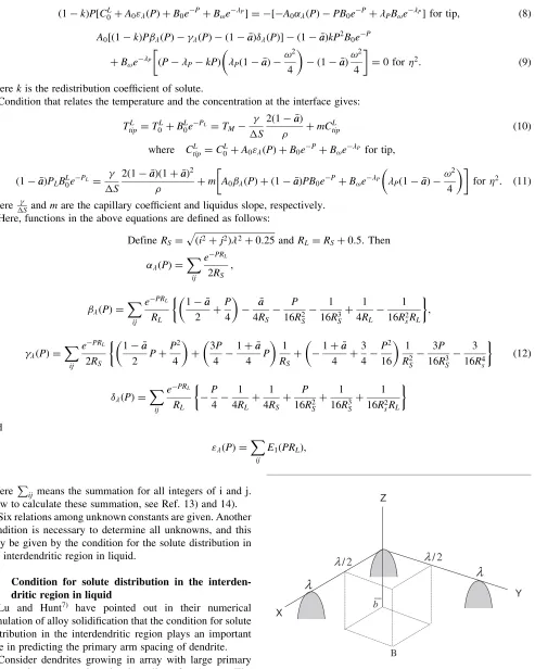
[image:2.595.72.267.71.238.2]The array is defined by dendrites which locate each other with dimensionless distance in ðx;yÞ plane as shown in Fig. 1.
3. Temperature and Concentration Field
The temperature field and solute one around the dendrite interface are governed by diffusion equations in coordinates moving with the tip.
r2TLþ2PL @TL
@z ¼0; r2TSþ2PS
@TS
@z ¼0; ð3Þ
r2CLþ2P @CL
@z ¼0:
In these,TLandTSare the temperature fields in liquid and in solid, respectively, andCL is the solute field in liquid. The parameters PL andPS are thermal Peclet numbers in liquid and in solid, respectively, andPis the solute Peclet number in liquid.
In order to simplify the discussions, we assume the thermal diffusion coefficient is very large compared to the solute one. This means the temperature change is very small in the scale of order of tip radius, . The temperature in solid will be determined by the temperature in liquid, through boundary conditions at interface, because the heat flows from liquid to
solid in the constrained growth. The solute diffusion coefficient in solid is assumed to be very small compared to one in liquid. These assumptions conclude that the growth of dendrite/cell will be controlled by the distribution of temperature and solute in liquid.
The temperature in liquid13)could be described by
TL¼T0LþB
L
0e
2PLZ whereP
L¼ V
2L
ð4Þ
The solute distribution in liquid13)could be expressed by
CL¼C0LþA0
X
i;j
E1ðP2ijÞ þB0e2PZ
þB!e2PZ
1
2ðcosð!xÞ þcosð!yÞÞ ð5Þ where
P¼V
2D; !¼
2 ;
2ij¼
ffiffiffiffiffiffiffiffiffiffiffiffiffiffiffiffiffiffiffiffiffiffiffiffiffiffiffiffiffiffiffiffiffiffiffiffiffiffiffiffiffiffiffiffiffiffiffiffiffiffiffiffi ðxiÞ2þ ðyjÞ2þz2
q
þz
and
P ¼ 1 2ð
ffiffiffiffiffiffiffiffiffiffiffiffiffiffiffiffi P2þ!2
p
þPÞ:
E1ðxÞrepresents the integral exponential function.LandD are the thermal diffusivity in liquid and the solute one in liquid, respectively. In the summation for i and j, all integers will be summed, corresponding to neighboring dendrites, which include the dendrite itself at the origin of coordinate.
T0L;BL0;C0L;A0;B0andB!are constants to be determined.B0
-term in CL is introduced to study the effect of solute distribution in the interdendritic region on the dimensions of dendrite/cell.
3.1 Restrictions from boundary conditions
The simple approximation for the temperature field and the concentration field are given in eqs. (4) and (5). They include seven unknown constants, namelyTL
0;BL0;CL0;A0;B0;B!and
(the tip radius of curvature). These may be determined from boundary conditions. The other constant, , the dimension-less primary arm spacing, may be determined by the minimum undercooling criteria at the tip.
Here we consider a dendrite located at the origin of coordinate, whose tip coordinate is atðx;y;zÞ ¼ ð0;0;0:5Þ.
The solute concentration far from the tip in the liquid will be the initial average solute concentration,C0. This gives:
C0L¼C0: ð6Þ
Temperature gradient at the tip,GL, in the liquid is given:
GL¼ 1
@TL
@z ¼
2
PLB L
0e
PL: ð7Þ
In order to determine the tip radius of curvature, three points on the interface are, at least, needed. These points are chosen: one point at the tip and the other is very close to the tip with distance, r¼pffiffiffiffiffiffiffiffiffiffiffiffiffiffiffix2þy2, because of the axial
symmetry of the interface. This means all calculations should be carried out up to 2 (or r2¼x2þy2) for every boundary condition at the interface.
Mass conservation condition at the interface gives rela-tions among constants:
x,i y,j
ð1kÞP½CL0þA0"ðPÞ þB0ePþB!eP ¼ ½A0ðPÞ PB0ePþPB!ePfor tip; ð8Þ
A0½ð1kÞPðPÞ ðPÞ ð1aaÞ ðPÞ ð1aaÞkP2B0eP
þB!eP ðPPkPÞ Pð1aaÞ !2
4
ð1aaÞ!
2
4
¼0 for2: ð9Þ
wherekis the redistribution coefficient of solute.
Condition that relates the temperature and the concentration at the interface gives:
TtipL ¼T0LþBL0ePL ¼T
M
S
2ð1aaÞ
þmC
L
tip ð10Þ
where CLtip¼CL0þA0"ðPÞ þB0ePþB!eP for tip;
ð1aaÞPLBL0e
PL¼
S
2ð1aaÞð1þaaÞ2
þm A0ðPÞ þ ð1aaÞPB0e
PþB
!eP Pð1aaÞ !2
4
for 2: ð11Þ
whereSandmare the capillary coefficient and liquidus slope, respectively. Here, functions in the above equations are defined as follows:
DefineRS¼
ffiffiffiffiffiffiffiffiffiffiffiffiffiffiffiffiffiffiffiffiffiffiffiffiffiffiffiffiffiffiffiffiffiffiffiffi ði2þj2Þ2þ0:25
p
andRL¼RSþ0:5:Then ðPÞ ¼
X
ij
ePRL
2RS ;
ðPÞ ¼
X
ij
ePRL
RL
1aa 2 þ
P
4
aa
4RS
P
16R2
S
1
16R3
S
þ 1
4RL
1
16R2
sRL
;
ðPÞ ¼
X
ij
ePRL
2RS
1aa 2 Pþ
P2
4
þ 3P
4 1þaa
4 P
1
RS
þ 1þaa
4 þ 3 4 P2 16 1 R2 S 3P
16R3S
3 16R4
s
ð12Þ
ðPÞ ¼
X
ij
ePRL
RL
P
4 1 4RL
þ 1
4RS
þ P
16R2
S
þ 1
16R3
S
þ 1
16R2
sRL
and
"ðPÞ ¼
X
ij
E1ðPRLÞ;
wherePijmeans the summation for all integers of i and j. How to calculate these summation, see Ref. 13) and 14).
Six relations among unknown constants are given. Another condition is necessary to determine all unknowns, and this may be given by the condition for the solute distribution in the interdendritic region in liquid.
3.2 Condition for solute distribution in the
interden-dritic region in liquid
Lu and Hunt7) have pointed out in their numerical
simulation of alloy solidification that the condition for solute distribution in the interdendritic region plays an important role in predicting the primary arm spacing of dendrite.
Consider dendrites growing in array with large primary arm spacing compared to the tip radius of curvature. The diffusion length of solute will be small compared to the primary arm spacing, then the solute concentration in the bottom of liquid, the point B in the Fig. 2, will be very close to the initial concentration of the alloy.
In the description of solute distribution in liquid, eq. (5), the value of integral exponential function will quickly decrease withP2ijincreased. Then, the solute concentration should satisfy the condition,
B0e2P
b bB
!e2P
b
b¼0 ð13Þ
at the point B, in order the solute concentration to approach to the initial concentration. When the morphology is assumed to scale to the tip radius of curvature, the value ofbbshould be constant in the dimensionless coordinates. The relation, eq. (13), betweenB0andB!is used as a boundary condition
/2
λ
λ
/2b B X Y Z
λ
λ
[image:3.595.59.552.67.683.2]for calculations, though the constant bbis assumed to be a constant. (Note here eq. (13) means thatB!vanishes whenbb
approaches to the negative infinity, and then the solute distribution in liquid is described withoutB!-term in eq. (5)).
3.3 How to predict the tip radius of curvature and the
primary arm spacing
The temperature gradient in the liquid,GL, and the initial concentration of solute,C0, are given. And assume also that
the deviation parameter from the perfect paraboloid of
revolution, aa, and the parameter for liquid depth in the interdendritic region,bb, are constants.
The tip radius of curvature,, as a function of the growth rate,V, is calculated as follows:
From eq. (7), the constantBL
0 inTLcan be derived
BL0ePL ¼ GL
2PL
: ð14Þ
From eqs. (6), (8), (9) and (13), constantsA0;B!andB0in
CLare expressed by Peclet number
A0¼
ð1kÞPC0
ð1kÞP"ðPÞ ðPÞ þbP0½ð1kÞPPkPeð12 bbÞðPpÞ ;
B!eP¼bP0A0; ð15Þ
B0¼e2bðPPÞB!;
where
bP0 ¼ ð1kÞPðPÞ ðPÞ ð1aaÞ ðPÞ ðPPkPÞ
ð1aaÞP !2
4
ð1aaÞ!
2
4 ð1aaÞkP
2eð12 bbÞðPPÞ
:
Then, for a given dimensionless spacing the tip radius of curvature is calculated as follows:
(a) Assume the value of tip radius, (b) Calculate Peclet numbersP;PL,
(c) By eqs. (14) and (6), calculateBL0 andCL0.
(d) Calculate ðPÞ; ðPÞ; ðPÞ; ðPÞ and "ðPÞ in
eqs. (12), (e) DeterminebP
0, and getA0;B!andB0 from eqs. (15).
(f) InsertBL
0 andA0;B!;B0into eq. (11),
(g) When eq. (11) is satisfied, the value is tip radius corresponding to the given dimensionless spacing,. In other cases, repeat again the calculation for other value offrom steps (b) to (f).
(h) CalculateTL
0 by eq. (10).
3.4 How to select the dimensionless spacing and the
primary arm spacing
In order to select the dimensionless spacing, we assume the dendrite with minimum undercooling of tip will overgrow and survive. The undercooling of a tip of dendrite,Ttip, is
defined and expressed by using equation (10) as follows: Ttip¼TMþmC0TtipL
¼
S
2ð1aaÞ
mðC
L
tipC0Þ ð16Þ
¼
S
2ð1aaÞ
m½A0"ðPÞ þB0e P
þB!eP
Then, for a given growth rate and dimensionless spacing, (i) Calculate Ttip, and choose corresponding to the
minimumTtip value.
(i) Determine the primary arm spacing by
1 ¼:
4. Prediction and Comparison with Experiments
We shall now examine the calculated results obtained for
succinonitrile(SCN)-acetone solution and for Al-Cu alloy. The values of the parameters used in the calculations are shown in Table 1.
The deviation parameter, aa, for the tip shape of dendrite from the paraboloid of revolution is treated to be a constant parameter with same order of magnitude with the crystalline anisotropy of interfacial energy.11)Without deviation from
paraboloid, we have no solutions corresponding to dendr-ite(D-solution in the following sections). In the phase field model,9,10)the dendritic solutions do not exist without the
anisotropy of interfacial energy. Therefore, the deviation from paraboloid of revolution will root in and have a relation with the anisotropy of interfacial energy, though the details have not been studied.
The parameter,bb, for the interdendritic liquid depth will be assumed to be a parameter with same order of magnitude corresponding to the mushy zone length in the dendrite solidification.
[image:4.595.305.550.371.518.2]Calculated results are shown for SCN-1.0 mol%Acetone solution in the following sections.
Table 1 Parameters used in the calculations for SCN-Acetone solution and Al-Cu alloy.
Parameter Value
SCN-Acetone solution Al-Cu alloy
TM 331.24 (K) 933.6 (K)
m 2:16/K(mol%)1 2:50/K(mass%)1
S 6:16710
8(mK) 1:04107(mK)
D 1:27109(m2s1) 5:0109(m2s1)
k 0.103 0.140
L 1:134107(m2s1) 3:76105(m2s1)
C0 1.0 (mol%) 4.0 (mass%)
a
a 0.002 0.002
b
b 14:0 16:0
4.1 Behavior of solutions for a given dimensionless
spacing
We have two types of solutions: one type is a solution for small value, and the other is for large value.
The behavior of solutions with small is shown in Fig. 3(a) (we call these CD-type solutions) as functions of the growth rate, and one with large in Fig. 3(b) (D-type solutions). Solutions with small approach to a marginal solution with increasing value, and there transform to solutions with large value. With more increase of , solutions will approach to a limiting solution with ¼ 1. Solutions with small exist irrespective of the sign of the value of aa, but solutions with large exist only when the value ofaais positive.
At a given growth rate, the above solutions give a relation/ relations between the primary arm spacing,1ð¼Þ, and the
tip undercooling(Fig. 4). This figure shows that the tip undercooling has its local minimum value at some primary arm spacing.
4.2 Tip radius and the primary arm spacing
The needle with smaller tip undercooling is assumed to grow predominantly for others. Then the solution with minimum tip undercooling will represent a growing needle, and then the tip radius, primary arm spacing and the tip undercooling will be determined for the growing needle.
0.1 1 10
10–2 10–1 100
D–solution CD–solution
) /
10
(V= 4.0× –3mm sin1CDrange
Tip underco
oling
T
∆
tip
/K
Primary arm spacing, / mmsλ -1
(a)
10
(V= 4.0× –2mm / s in D range) 0.1
1 10
10–3 10–2 10–1 100
Tip undercooling
∆
Ttip
/K
Primary arm spacing, / mms-1
1
λ
(b)
1 1.1 1.3 1.5 1.7 1.9
10–3
10–2
10–1
Tip undercooling
∆
Ttip
/K
Primary arm spacing, / mms-1
1
λ
) /
10
(V= 4.0× –1mm sinupper CDrange
(c)
Fig. 4 Dimensions given by minimum tip undercooling criteria: (a) Tip radius of curvature and primary arm spacing with growth rate. C, CD and D show different growth range(see text). (c) Tip undercooling with growth rate.
10–4
10–3
10–2
10–1
100
10–4 10–3 10–2 10–1 100 101
Growth rate V /mms-1
Lam=10 Lam=15 Lam=20 Lam=30 λ
Tip radius
/mm
ρ
(a)
10–4
10–3
10–2
10–1
100
10–4 10–3 10–2 10–1 100 101
Growth rate V /mms-1
40 200 1000 10000 λ
Tip radius
/mm
ρ
(b)
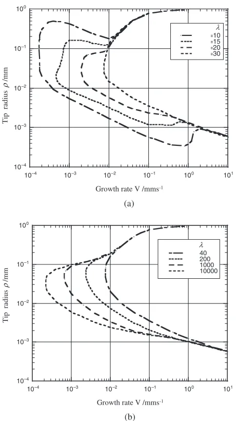
[image:5.595.325.526.43.651.2] [image:5.595.55.285.69.479.2]The variation of the tip radius of curvature, the primary arm spacing and the tip undercooling with growth rate are shown in Fig. 5(a) and (b).
The CD-type solutions and the D-type solutions have their own local minimum value of tip undercooling, giving almost same value of tip radius of curvature. The typical points are: . In the low growth rate and also in the high growth rate, the CD-type solution alone has the minimum value of tip undercooling, Ttip(we call this solution
CD-solu-tion), as can be seen in the growth range C in Fig. 4. . In the middle growth rate the D-type solution has its
minimum value of tip undercooling,Ttip(D-solution),
and within some growth range the CD-solution dis-appears(in the growth range D in Fig. 4).
. And, in some range of growth rate the minimum of CD-solution co-exist with the minimum of D-CD-solution(in the
growth range CD in Fig. 4). And CD-solution gives almost same value of undercooling of tip with that given by D-solution(Fig. 4(b)).
. The predicted primary arm spacing by D-solution shows the divergence at the marginal growth rate. This divergence owes to the different dependency of the capillary effect and the solute concentration on. Predicted tip radius of curvature and primary arm spacing show very similar dependency with those observed exper-imentally. CD-solution may represent the cellular morphol-ogy and D-solution the dendritic one. In the next section we study this from the constitutional supercooling around the tip of needle.
4.3 Constitutional supercooling in ðx;yÞ plane around
the tip of needle
Here, we study the behavior of supercooling in (x,y)-plane (plane perpendicular to the growth direction), which includes the tip of needle. We define the temperature given by thermal field, Ttherm, and the constitutional one given by the solute
distribution,Tcon, by
Tcon¼TMþmCL: ð17Þ
The supercooling, Tsup, is defined by the difference betweenTtherm andTconby
Tsup ¼TconTtherm: ð18Þ
Figure 6 shows the supercooling,Tsup, in theðx;yÞplane: one is the supercooling in x-direction with dimensionless distance from the tip and the other shows the supercooling tilted 45 degree from x-direction in (x,y) plane. In the two directions, supercoolings given by the CD-solution (Figure 6(a), V¼1:0103mm/s) have very similar
de-pendency on the distance, showing the axsymmetric super-cooling. But for those given by the D-solution(Fig. 6(b),
V ¼4:0102mm/s), the supercooling given in the
direc-tion tilted 45 degree from x-direcdirec-tion has larger supercooling than that in the x-direction.
Larger the supercooling, then larger instability of the interface would be. Then the interface will grow in the direction with larger supercooling. Therefore the interface given by D-solution will have the morphology like a dendrite.
4.4 Effects of the interfacial shape and liquid depth in
the interdendritic region on dimensions
The interface shape is assumed to be deviated from the perfect paraboloid of revolution.
The more deviation from parabola makes the growth range of D-solution broader and the primary arm spacing smaller, but a little effect on of CD-solution. The critical growth rate from D-solution to CD-solution (corresponding to the divergence of primary arm spacing) becomes large when the deviation becomes significant.
The solute concentration in the interdendritic region is assumed to be very close to the average solute concentration,
CL¼C0 at a point ðx;y;zÞ ¼ ð=2; =2;bbÞ. The change of
this parameter affects the growth range of CD-solution: the smaller value of the parameter,bb, makes the growth range of CD-solution broader.
10–5
10–4
10–3
10–2
10–1
100
101
102
103
10–4 10–3 10–2 10–1 100 101 102
D-sol
1 λ
1 λ
1 λ
ρ
Dimension
ρ
,
λ1
/mm
Growth rate V /mms-1
C CD D CD C
CD-sol
(a)
10–1
100
101
102
10–4 10–3 10–2 10–1 100 101 102
D-sol.
CD-sol.
Growth rate V /mms-1
Tip undercooling
∆
Ttip
/K
(b)
Fig. 5 Variation of tip undercooling with primary arm spacing. Tip undercooling has a locally mimimum value (by*) at some primary arm spacing. (a) AtV¼4:0103mm/s(in the growth range of CD),
CD-type solution and D-CD-type one have its own minimum tip undercooling. (b) AtV¼4:0102mm/s(in the growth range of D), CD-type solution
continuously transforms to D-type one, and has a minimum tip under-cooling. (c) AtV¼4:0101mm/s(in the growth range of CD),
[image:6.595.58.279.72.459.2]4.5 Comparison with experimental results
Predictions for SCN-1.0 mol%Acetone solution are com-pared with experimental results for the tip radius of curvature and primary arm spacing15)in Fig. 7(a). Calculations are also applied to the Al-4.0 mass%Cu alloy and compared with experimental results16)in Fig. 7(b). Deformation parameteraa and the depth parameter of liquidbbin the prediction for Al-Cu alloy are adopted almost same values as those used in the calculation for SCN-acetone solution. Correspondence be-tween predictions and experimental results are shown very well both for the tip radius of curvature and the primary arm spacing.
5. Summary and Discussion
Tip radius of curvature of dendrite/cellular interface and primary arm spacing are predicted and compared with experimental results for the solidification of SCN-acetone solution and Al-Cu alloy, and the correspondences are shown very well.
In the model, a small deformation of interfacial shape from parabolic one is allowed, then two types of solution, CD-type
solution and D-type solution, are given. Among solutions of dimensions, minimum tip undercooling criteria is applied to select a growing solution.
CD-solution is given in the low growth rate and also in the high growth rate. D-solution is given in the middle growth rate. Predicted primary arm spacing by D-solution diverges at some high growth rate, and this critical growth rate depends on the magnitude of deviation parameter from parabola. Csolution will correspond to the cellular morphology and D-solution to dendrite one, because of their dependency of dimensions on the growth rate.
At some growth rate, two types of solutions co-exist, and whose tip undercoolings are predicted to be almost same. Therefore, a new selection rule/criteria will be needed other than minimum tip undercooling to select a growing solution. Larger deformation from parabola is shown to make the growth range of D-solution broader, and to make the critical growth rate larger, which corresponds to the divergence of primary arm spacing.
Liquid depth parameter, which will correspond to the mushy zone, affects little to dimensions given by D-solution, but changes the growth range of CD-solution. The liquid depth parameter should be determined experimentally by the
10–3
10–2
10–1
100
101
10–3
10–2
10–1
100
Dimension
ρ
,
λ1
/mm
Growth rate V /mms-1 ρ
1
λ
mm K GL=2.2 /
mm K GL=2.6 /
(a)
10–4
10–3
10–2
10–1
100
101
10–3 10–2 10–1 100 101
1 λ
1 λ
1 λ
ρ
Growth rate V /mms-1
Dimensi
on
ρ
,
λ1
/mm
mm K GL=4.0 /
(b)
Fig. 7 Predicted tip radius of curvature and primary arm spacing. (a) SCN-1.0 mol%Acetone solution. Squares show data with GL¼2:60:2K/
mm and triangles do withGL¼2:20:4K/mm. (b) Al-4.0 mass%Cu
alloy(GL¼4:00:4K/mm). 0
0.1 0.2 0.3 0.4 0.5 0.6
0 5 10 15 20 25 30
x–dir xy–dir
Dimensionless distance from tip
Supercooling
∆
Tsup
/K
(a)
0 0.1 0.2 0.3 0.4 0.5 0.6
0 5 10 15 20 25 30
x–dir xy–dir
Dimensionless distance from tip
Supercooling
∆
Tsup
/K
(b)
[image:7.595.329.524.70.435.2] [image:7.595.69.269.71.438.2]critical growth rate of transition from the cellular to the dendrite interface.
REFERENCES
1) B. Chalmers: Principles of Solidification, (Wiley, New York, NY, 1964) pp. 126–185.
2) T. F. Bower, H. D. Brody and M. C. Flemings: Trans. AIME236(1960) 624–634.
3) M. H. Burden and J. D. Hunt: J. Cryst. Growth22(1974) 99–108. 4) M. H. Burden and J. D. Hunt: J. Cryst. Growth22(1974) 109–116. 5) R. Trivedi: J. Cryst. Growth49(1980) 219–232.
6) W. Kurz and D. J. Fisher: Acta Metall.29(1981) 11–20. 7) S.-Z. Lu and J. D. Hunt: J. Cryst. Growth123(1992) 17–34.
8) U. Bisang and J. H. Bilgram: Phys. Rev.42(1996) 5309–5326. 9) A. A. Wheeler, W. J. Boettinger and G. B. McFadden: Phys. Rev. A45
(1992) 7424- .
10) S. G. Kim, W. T. Kim and T. Suzuki: Phys. Rev. E60(1999) 7186- . 11) M. E. Glicksman and S. P. Marsh:Handbook of Crystal Growth, ed. by
D. T. J. Hurle, vol. 1B, Chap. 15(Elsevier Science Pub., 1993). 12) Y. Miyata, M. E. Glicksman and S. H. Tirmizi: J. Cryst. Growth110
(1991) 683–691.
13) Y. Miyata and M. Takeda: Mater. Trans.42(2001) 180–188. 14) Y. Miyata and M. Takeda: Mater. Trans.42(2001) 189–196. 15) Y. Miyata, H. Takahashi and M. Herai: Submitted to J. Japan Inst.
Metals.