Output effects of fiscal stimulus in Central and Eastern European Countries

Munich Personal RePEc Archive

Output effects of fiscal stimulus in

Central and Eastern European Countries

Combes, Jean Louis and Minea, Alexandru and YOGO,

Thierry and Mustea, Lavinia

CERDI-Université d’Auvergne, CEREG-University of Yaoundé

31 April 2015

Online at

https://mpra.ub.uni-muenchen.de/65623/

Output Effects of Fiscal Stimulus in

Central and Eastern European Countries

Jean-Louis Combes*, Alexandru Minea*@, Lavinia Mustea*& and Thierry Yogo*

Abstract: In spite of the rapidly growing research on fiscal multipliers

over the recent years, little evidence has been so far accumulated in

developing and emerging economies. This paper investigates the nature

and the size of fiscal multipliers in Central and Eastern European

Countries (CEEC). Unlike most of existing literature, we draw upon a

panel vector error correction model, which appropriately captures the

common long-term path of CEEC, while allowing for different short-run

dynamics, in an integrated setup. Our main results show that the spending

multiplier is positive, but low on average. Moreover, its sign, significance

and magnitude vary across CEEC. Finally, both impulse and cumulative

fiscal multipliers are sensitive to a wide range of CEEC characteristics,

including the exchange rate regime, the level of economic development,

the fiscal stance, and the openness degree.

JEL Classification: E62, O11, P35

Keywords: Central and Eastern European Countries; fiscal multipliers;

panel vector error correction model.

*

CERDI & School of Economics, University of Auvergne, 65 Bd. Fr. Mitterrand, B.P. 320, 63009 Clermont-Ferrand, France.

&

Faculty of Economics and Business Administration, West University of Timisoara, Romania.

@

I. Introduction

The fiscal multiplier has received a renewed attention since the recent financial crisis

and the widespread fiscal stimulus implemented by many countries around the world. In spite

of the rapidly growing research on fiscal multiplier over the recent years, so far little evidence

has been accumulated in emerging and developing economies.1

In this paper, we develop the literature by investigating the effect of discretionary

fiscal change on economic activity in 11 Central and Eastern European Countries (CEEC).

CEEC share some specific characteristics that may affect the multiplier. Specifically, they are

relatively small open economies with relatively low debt levels, and are currently

implementing structural reforms that are more or less correlated with the accession to the

European (Monetary) Union (E(M)U). In this respect, assessing the nature and the size of the

effects of fiscal stimulus is of great interest to implement a more tailored fiscal policy.

The contribution of our paper is fourfold. First, unlike the existing literature that relies

extensively on VAR models, our analysis uses a Panel Vector Error Correction model

(PVECM), selected for its appealing features for CEEC. Indeed, on the one hand, all CEEC in

our sample are expected to follow a common dynamic in the long-term, driven by their

integration process in the E(M)U. As such, drawing upon methods that remove this long-term

dynamic (for example, through first-differentiation, as this is the case in stationary VAR

models), would significantly affect the estimation of fiscal multipliers. On the other hand,

albeit following a common long-run path, CEEC may present different short-run dynamics.

Models that do not account for such country-heterogeneities (such as PVAR) or abstract of

the common long-run path (such as individual country-estimated VAR) are equally likely to

produce biased estimations of fiscal multipliers. Consequently, unlike most studies, we take

full advantage of the statistical properties of the data, and particularly of co-integration

between variables, by using an error correction model on a panel data setting. This

methodology is appropriate for computing both pooled and country-specific fiscal multipliers

within the same framework, while controlling for the common long-run relationship between

CEEC.

Second, a crucial issue is related to the identification of truly exogenous fiscal shocks.

However, most VAR models rely upon a simple Cholesky-decomposition of shocks, in which

identification arises from the ordering of variables. In this paper, we draw upon Fatas and

Mihov (2003, 2006), Afonso et al. (2010) and Agnello et al. (2013), and define spending

1

shocks as the cyclically-adjusted component of government spending. By so doing, we isolate

an unexpected change in fiscal policy as the source of fiscal shocks.

Third, we employ genuine (i.e. not interpolated) quarterly data for the period

1999q1-2013q3. The use of quarterly data to compute multipliers is extremely rare: if we take into

account the VAR-based literature, Ilzetzki et al. (2013) is such an example. These authors

state that the use of quarterly data is useful for identifying shocks properly. In addition,

compared to Ilzetzki et al. (2013), we exploit only one source to collect quarterly data, which

ensures homogenous data for our panel of CEEC.

Fourth, after presenting pooled and country-specific multipliers, we explore the

sensitivity of the effect of fiscal policy by disentangling CEEC across several of their major

characteristics, namely the exchange rate regime (ERR), the level of economic development,

the fiscal stance, and the openness degree.

Our results are as follows. First, we find that impact and four-quarter cumulative

multipliers are positive and significant for CEEC. Although the size of impact multipliers is

fairly small, namely between 0.07 and 0.09 (depending on the estimation method), cumulative

multipliers can be up to four times higher compared to impact multipliers, namely between

0.21 and 0.31. Second, we unveil significant differences among fiscal multipliers across

CEEC. Although positive in most countries, impact and cumulative multipliers can be

statistically not significant or even negative in some CEEC. In addition, the magnitude of

cumulative multipliers differs by a factor of four between CEEC, and climbs up to a large

value of 0.7. Third, we show that not accounting for a common (instead of

country-individual) long-term path can leave to important significance and size differences for fiscal

multipliers in several CEEC of our sample. Finally, both impact and cumulative fiscal

multipliers are sensitive to CEEC specificities. Albeit the ERR is found to be unimportant for

output’s response to fiscal shocks on impact, the ERR affects its cumulative response; in

particular, cumulative multipliers are significant in pegged and floating ERR, and not

significant in intermediate ERR. Next, both impact and cumulative multipliers are mainly

significant in relatively less developed CEEC and in CEEC with relatively lower debt-to-GDP

ratios. Finally, consistent with the predictions of the Mundell-Fleming model, we find that

cumulative multipliers are significant only in relatively less open CEEC.

The rest of the paper is structured as follows. Section II summarizes the findings of

previous studies. Section III presents the data and outlines the methodology. Section IV

illustrates the main results. Section V discusses the sensitivity of fiscal multipliers to several

II. Literature review

The major fiscal stimuli implemented by governments in response to the recent crisis

reopened the topic of the multiplier in academia.2 As pioneered by Keynes (1936), the

multiplier predicts a more than 1 to 1 change in GDP following a fiscal shock. However, as

emphasized by Blanchard and Leigh (2013), the IMF was significantly under-evaluating fiscal

multipliers. According to Marglin and Spiegler (2013), such conflicting findings are

engendered by the use of different methodologies, time span, type of government spending,

and, according to Chahrour et al. (2012), different identification methods for fiscal shocks.

Indeed, the literature devoted to the estimation of fiscal multipliers is particularly rich,

and involves the use of many methods. Theoretically, fiscal multipliers can be approached

using (i) the ISLM model in its static (Hicks, 1937) and dynamic (Blanchard, 1981) forms, (ii)

RBC models, developed under the New Classical economics (Long and Plosser, 1983), and

(iii) New Keynesian DSGE models (Gechert and Will, 2012). Econometrically, fiscal

multipliers can be computed using (i) the Narrative Approach (Romer and Romer, 2010), (ii)

the Vector AutoRegression (VAR) models (Blanchard and Perotti, 2002), (iii)

single-equations models (Barro and Redlick, 2009), (iv) instrumental variables (Nakamura and

Steinsson, 2014), (v) panel models (Almunia et al., 2010), and (vi) two-stage residual

techniques (Agnello et al., 2013).

Due to the large strand of literature that focused on estimating fiscal multipliers, we

present in the following the results of the studies that are the closest to our paper, by focusing

on developing countries. Based on the estimation of elasticities and regressions to isolate

fiscal shocks, IMF (2008) illustrates spending multipliers of 0.2 (-0.2) after one (two) years.

Such low spending multipliers equally emerge from the PVAR analysis of Ilzetzki & Végh

(2008), performed on 27 developing countries, namely 0.6/0.4/0.1 on impact/1st/2nd year.

More recently, Kraay (2012, 2014) finds a spending multiplier of 0.5 (0.4) based on a sample

of 29 (102) developing countries, while Ilzetzki et al. (2013) find public consumption

multipliers equal to -0.03 (0.4) on impact (after 4 quarters). Finally, Minea & Mustea (2015)

reveal short-lived impact and short-run fiscal multipliers for developing Asian and African

Mediterranean countries. Overall, these studies emphasize that fiscal multipliers are fairly low

in developing countries.

2

III. Data and Methodology

We aim at empirically assessing output effects of a discretionary fiscal policy in CEEC. We

begin by presenting the data, and then we expose the methodology.

3.1. Data

We use quarterly data for a sample of 11 CEEC over the period 1999q1-2013q3 (see Tables

A.1a-b in Appendix for the list of countries and descriptive statistics).3 Except for Central

Government debt, which is measured by the quarterly public sector debt of the World Bank,

all data are from EUROSTAT.

Two main reasons justify the choice of quarterly data. First, as compared to annual

data, the use of quarterly data is crucial for capturing the fact that fiscal authorities can

respond to output shocks as rapidly as only after one quarter (Ilzetzki et al., 2013). Second,

quarterly data provide a substantial increase in the number of degrees of freedom compared to

annual data, an important feature given the relative small time span usually available for

European post-communist economies (hardly 15 years, in our study). In particular, as pointed

out by Ilzetzki et al. (2013), interpolated quarterly data may lead to spurious regressions

since, by construction, the interpolation creates a strong correlation between government

spending and output. Thus, we use only genuine quarterly data, namely data that were

originally collected at quarterly frequency.4

Our main variables are the gross domestic product (GDP), the total government

expenditure, defined as the sum of the general government final consumption and gross fixed

capital formation, and taxes, which include taxes on imports and exports less subsidies. Prior

to their use in regressions, all variables are deflated by the consumer index (CPI) and

seasonally adjusted using a moving-average filter.

3.2. Time series properties of variables

We explore time series properties of variables using three types of panel unit root

tests. On the one hand, the Augmented Dickey Fuller (ADF) Fisher-type test of Choi (2001)

and the Im, Pesaran and Shin (IPS, 2003) unit root test, which both assume the null

hypothesis that all panels contain a unit root against the alternative of at least one stationary

3

Although collected data cover the period 1992q2-2013q3, our sample starts in 1999q1 for several reasons. First, we allow CEEC to stabilize from the major imbalances engendered by the end of the Cold War. Second, we obtain a balanced sample with data collected at quarterly frequency.

4

panel. Compared to alternative tests (such as Levin, Lin and Chu, 2002), these tests present

the advantages of allowing the autoregressive parameter to be country-specific and of not

requiring panels to be strongly balanced. On the other hand, to account for the presence of a

relatively weak number of countries and time dimension, which is inherent when analyzing

CEEC, we equally draw upon the Levin, Lin and Chu (2002) unit root test.

Provided variables are integrated of the same order, we test in the following for

cointegration. For this purpose, we revert to the cointegration tests coined by Westerlund

(2007), which extend to panel data the time series test of Banerjee et al. (1998). These tests

assume the null hypothesis of no cointegration. In particular, compared to alternative tests

(such as, for example, the residual-based test of Pedroni, 2004), Westerlund (2007) tests were

selected on the basis of allowing individual short-run dynamics and for remaining consistent

in the presence of possibly serial-correlated errors and weak exogenous regressors.

3.3. The econometric model

In this sub-section, we discuss the error correction specification and the choice of the

appropriate estimator. The use of the error correction framework can be justified both

empirically and theoretically.

Empirically, the choice of the appropriate model strongly depends upon the statistical

properties of the data. The existing literature on fiscal multipliers extensively resorts to the

VAR methodology, either with country or panel data. However, the use of an error correction

model is suitable when series are non stationary and cointegrated, as this is the case in our

analysis.

From a theoretical standpoint, it is not unreasonable to assume that the effect of fiscal

policy on output is not independent of the speed of adjustment to the long-run equilibrium, all

the more given the common long-term path of CEEC, driven by their integration process in

the E(M)U (see Nenovsky and Villieu, 2011). Therefore, it is suitable to account for the

long-run equilibrium when assessing the response of output to the fiscal impulse.

In line with Pesaran et al. (1999), we assume an autoregressive distributed lag model

(ARDL), with p lags for the dependent variable and q lags for each of the RHS variables

it i q

j

j it ij p

j

j it ij

it gdp x

gdp = α + δ +µ +ε =

− =

− 0 1

' , (1)

with i=1,N countries, t=1,T periods, gdp the log of real GDP, x_it the vector of

country-specific fixed effects, and ε_it the error term. Since our goal is to evaluate the effect of

government spending on output, it is necessary to include taxes as a control variable, as

spending are not independent of taxes (Blanchard and Perotti, 2002).5

Assuming that variables are I(1) and cointegrated, we reparameterise model (1) into

the following error correction model (Pesaran et al., 1999)

(

)

q j j it ij p j j it ij it i it i

it gdp x gdp x

gdp =φ −β + α ∆ + δ ∆ +µ +ε

∆ − = − − = − − 1 0 * 1 1 *

1 ' ' , (2)

where =− −

= p j ij i 1 1 α

φ , = −

= k

ik q

j ij

i δ α

β / 1

0 , + = − = p j m im ij 1 * _α

α , and

+ = − = q j m im ij 1 * _δ

δ . The

first part of (2)–in levels–captures the long-run relationship, while the second part–in

differences–illustrates the short-run adjustment to the long-run equilibrium. Parameter φ_i is

the error-correcting term and measures the speed of adjustment. To validate the existence of a

long-run relationship, this parameter should be negative and significant.

The literature suggests three main approaches for the estimation of model (2): (i) the

dynamic fixed effect (DFE) estimator uses pooled data and allows the intercept to differ

across groups; however, if the assumption of the common slope fails to hold, then the

estimator is inconsistent; (ii) the pooling mean group estimator (PMG) combines both pooling

and averaging; it assumes long-run coefficients to be equal across groups, but allows

short-run coefficients to differ across groups, and (iii) the mean group (MG) estimator, which

allows intercepts, slope coefficients and errors variances to differ across groups (Pesaran and

Smith, 1995). In this paper, since we aim at capturing long-term dynamics, we start by using

the DFE estimator. Then, we draw upon previous evidence and econometric tests to make the

case for the use of the PMG estimator as the most appropriate for our sample of CEEC.

Indeed, the use of the PMG estimator will allow assessing the short-run dynamic of countries,

while controlling for the long-run relationship between spending and output.

3.4. Building a measure of discretionary expenditure shocks

The main feature of the error correction model (2) is that short-run dynamics of variables are

influenced by deviations from the long-run equilibrium. Thus, short-run coefficients capture

output’s responsiveness to fiscal policy adjustments with respect to the long-run equilibrium.

5

However, there is no reason to believe that observed variations in fiscal policy are exogenous

or unexpected. Thus, to compute output’s response to unexpected government spending

changes, we follow the methodology of Fatas and Mihov (2003, 2006), Afonso et al. (2010)

and Agnello et al. (2013), and construct a measure of discretionary fiscal policy as follows.

Assuming that public spending can be decomposed into a structural (anticipated) and a

residual (non-anticipated) component, we define discretionary spending shocks as the

cyclically-adjusted component of government spending, which reflects unexpected fiscal

policy changes. For each of 11 CEEC in our sample, we estimate the following model using

quarterly data over the period 1999q1-2013q3

( )

(

)

log , (3)

with G total government spending, ogap the output gap (based on the

Hodrick-Prescott-filtered log of real GDP), debt the central government debt in % of GDP, and trend the time

trend. Consequently, we capture spending shocks through the residuals ε.

Equation (3) differs from the specification of Fatas and Mihov (2003) and Agnello et

al. (2013). Indeed, following Blanchard (1993), and closely related Fatas and Mihov (2006),

we estimate equation (3) in levels. In addition, compared to Fatas and Mihov (2006) who use

GDP growth, we employ the output gap to capture the business cycle, for the following

reasons. Output gap has the advantage of controlling for the degree of inflation pressure.

Next, it also captures the state of unemployment, because a zero output gap corresponds to

full employment. Moreover, a negative output gap suggests the existence of available excess

capacities, while the crowding-out of private investment may be independent of the sign of

the GDP growth rate. Finally, we control for fiscal policy sustainability and for the

persistence of the responsiveness of fiscal policy to the business cycle, using the debt-to-GDP

IV. Fiscal multipliers in CEEC: Main results

4.1. Stationarity and cointegration

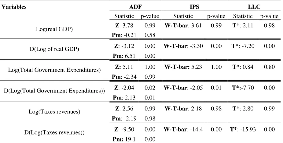
To assess the stationarity of our main variables, we report in Table 1 the results of the

Fisher-ADF, IPS and LLC unit root tests. We include in the auto-regressive specification of each test

both the trend and the intercept, to test for both difference and trend stationarity. As illustrated

by Table 1, the log of real GDP, total government expenditure and tax revenues are

nonstationary, since, irrespective of the test, we cannot reject the null hypothesis of the

presence of a unit root. In addition, as emphasized by low p-values, these variables are

stationary in first-difference, once again irrespective of the considered test. Since variables are

integrated of the same order, we look in the following for potential cointegration relations

among them.

Table 1: Unit root tests

Variables ADF IPS LLC

Statistic p-value Statistic p-value Statistic p-value Z: 3.78 0.99 W-T-bar: 3.61 0.99 T*: 2.11 0.98 Log(real GDP)

Pm: -0.21 0.58

Z: -3.12 0.00 W-T-bar: -3.30 0.00 T*: -7.20 0.00 D(Log of real GDP)

Pm: 6.51 0.00

Z: 5.11 1.00 W-T-bar: 5.23 1.00 T*: 0.84 0.80 Log(Total Government Expenditures)

Pm: -2.34 0.99

Z: -2.04 0.02 W-T-bar: -2.05 0.01 T*:-7.70 0.00 D(Log(Total Government Expenditures))

Pm: 2.13 0.01

Z: 2.56 0.99 W-T-bar: 2.18 0.98 T*: 2.80 0.99 Log(Taxes revenues)

Pm: -2.19 0.98

Z: -9.50 0.00 W-T-bar: -14.4 0.00 T*: -15.93 0.00 D(Log(Taxes revenues))

Pm: 19.1 0.00

Note: Z is the inverse normal statistic, Pm is the modified inverse chi-squared. The null hypothesis is “all panel contain a unit root”. The specification includes a trend and an intercept. We use 4 lags following the AIC test.

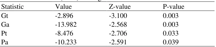
To assess cointegration, we draw upon Westerlund’s (2007) tests. These tests assume

the null hypothesis of no cointegration, against four different specifications of the alternative

hypothesis: the group mean test and its asymptotic version, which consider the alternative

hypothesis that the panel is cointegrated as a whole, and the panel mean test and its

asymptotic version, which consider the alternative hypothesis that there is at least one

cross-section unit for which the series are cointegrated. To preserve the consistency and the size

1000 replications. Table 2 provides the results of testing for a potential cointegration

relationship between real GDP, government expenditure and taxes. Irrespective of the

considered test, low p-values in Table 2 support the presence of cointegration between

variables.

Table 2: Westerlund (2007) cointegration tests

Statistic Value Z-value P-value

Gt -2.896 -3.100 0.003

Ga -13.982 -2.568 0.003

Pt -8.476 -2.706 0.033

Pa -10.233 -2.591 0.039

Note: Gt and Pt are respectively the group mean test and the panel mean test. Ga and Pa refer to the asymptotic version of the test. The null hypothesis is “no cointegration”. We use 3 lags following the AIC test.

Given that series in level are all I(1) and co-integrated, we will draw in the following

upon an error correction models to compute output’s response to spending shocks.

4.2. Fiscal multipliers in CEEC countries: full sample

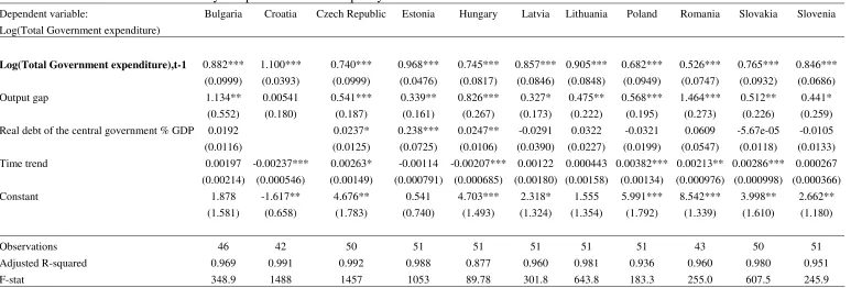
To estimate fiscal multipliers, we proceed in three steps. First, we isolate public spending

shocks. Table 3 illustrates the results of the OLS estimation of equation (3), for each of the 11

CEEC in our sample.6 As signalled by positively-significant coefficients of output gap,

government expenditure is pro-cyclical in all (but Croatia) CEEC in our sample, consistent

with previous evidence on developing and emerging countries (see Dalic, 2013). Furthermore,

non significant or positive debt coefficients suggest that the adjustment in response to

indebtedness takes place more likely through an adjustment of taxes than of public spending.

Finally, irrespective of the considered country, fairly high R2 values support the quality of our

specification for purging most of anticipated public spending, and isolate public spending

shocks through the country-specific error terms.

6

Table 3: Estimates of the discretionary component of the fiscal policy

Dependent variable: Bulgaria Croatia Czech Republic Estonia Hungary Latvia Lithuania Poland Romania Slovakia Slovenia Log(Total Government expenditure)

Log(Total Government expenditure),t-1 0.882*** 1.100*** 0.740*** 0.968*** 0.745*** 0.857*** 0.905*** 0.682*** 0.526*** 0.765*** 0.846*** (0.0999) (0.0393) (0.0999) (0.0476) (0.0817) (0.0846) (0.0848) (0.0949) (0.0747) (0.0932) (0.0686) Output gap 1.134** 0.00541 0.541*** 0.339** 0.826*** 0.327* 0.475** 0.568*** 1.464*** 0.512** 0.441*

(0.552) (0.180) (0.187) (0.161) (0.267) (0.173) (0.222) (0.195) (0.273) (0.226) (0.259) Real debt of the central government % GDP 0.0192 0.0237* 0.238*** 0.0247** -0.0291 0.0322 -0.0321 0.0609 -5.67e-05 -0.0105 (0.0116) (0.0125) (0.0725) (0.0106) (0.0390) (0.0227) (0.0199) (0.0547) (0.0118) (0.0133) Time trend 0.00197 -0.00237*** 0.00263* -0.00114 -0.00207*** 0.00122 0.000443 0.00382*** 0.00213** 0.00286*** 0.000267

(0.00214) (0.000546) (0.00149) (0.000791) (0.000685) (0.00180) (0.00158) (0.00134) (0.000976) (0.000998) (0.000366) Constant 1.878 -1.617** 4.676** 0.541 4.703*** 2.318* 1.555 5.991*** 8.542*** 3.998** 2.662**

(1.581) (0.658) (1.783) (0.740) (1.493) (1.324) (1.354) (1.792) (1.339) (1.610) (1.180)

Observations 46 42 50 51 51 51 51 51 43 50 51

Adjusted R-squared 0.969 0.991 0.992 0.988 0.877 0.960 0.981 0.936 0.960 0.980 0.951 F-stat 348.9 1488 1457 1053 89.78 301.8 643.8 183.3 255.0 607.5 245.9

Second, we use these recovered shocks as a measure of unanticipated public spending

in the estimation of the error correction model. However, drawing upon residuals from

another equation in the error correction model may lead to biased estimates. Therefore, we

correct standard errors using the Jackknife resampling procedure, which consists of repeatedly

computing standard errors, by omitting each time one observation.7 In our specific case, to

take into account both individual and time variability, the statistics are computed leaving out

one country.8

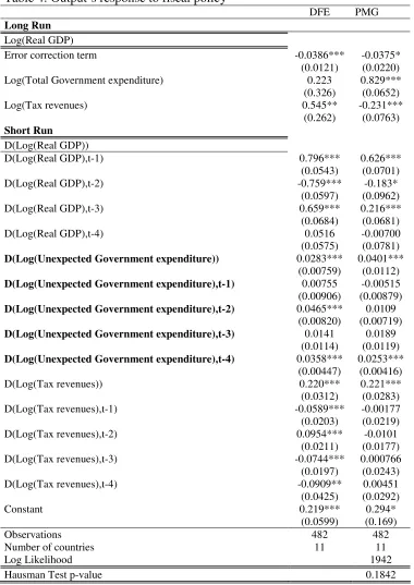
The first column of Table 4 reports the results of the error correction model used to

compute the effects of unanticipated public expenditure on output for the full sample of 11

CEEC, based on the dynamic fixed effect (DFE) estimator with four lags, as suggested by

AIC tests. Several points must be highlighted. The error correction term is significant and

negative, thus supporting our modelling strategy. Next, the fourth lag of unexpected

expenditure is significant, consistent with the tests for the choice of the optimal lag. Finally,

our strategy of controlling for tax revenues is supported by their significant coefficients.

Based on this model, we compute in the following fiscal multipliers.

7

Note that performing a standard bootstrap would underestimate time variability in our analysis.

8

Table 4: Output’s response to fiscal policy

DFE PMG

Long Run Log(Real GDP)

Error correction term -0.0386*** -0.0375* (0.0121) (0.0220) Log(Total Government expenditure) 0.223 0.829***

(0.326) (0.0652) Log(Tax revenues) 0.545** -0.231***

(0.262) (0.0763) Short Run

D(Log(Real GDP))

D(Log(Real GDP),t-1) 0.796*** 0.626*** (0.0543) (0.0701) D(Log(Real GDP),t-2) -0.759*** -0.183* (0.0597) (0.0962) D(Log(Real GDP),t-3) 0.659*** 0.216***

(0.0684) (0.0681) D(Log(Real GDP),t-4) 0.0516 -0.00700 (0.0575) (0.0781) D(Log(Unexpected Government expenditure)) 0.0283*** 0.0401***

(0.00759) (0.0112) D(Log(Unexpected Government expenditure),t-1) 0.00755 -0.00515 (0.00906) (0.00879) D(Log(Unexpected Government expenditure),t-2) 0.0465*** 0.0109

(0.00820) (0.00719) D(Log(Unexpected Government expenditure),t-3) 0.0141 0.0189

(0.0114) (0.0119) D(Log(Unexpected Government expenditure),t-4) 0.0358*** 0.0253***

(0.00447) (0.00416) D(Log(Tax revenues)) 0.220*** 0.221*** (0.0312) (0.0283) D(Log(Tax revenues),t-1) -0.0589*** -0.00177 (0.0203) (0.0219) D(Log(Tax revenues),t-2) 0.0954*** -0.0101 (0.0211) (0.0177) D(Log(Tax revenues),t-3) -0.0744*** 0.000766

(0.0197) (0.0243) D(Log(Tax revenues),t-4) -0.0909** 0.00451 (0.0425) (0.0292)

Constant 0.219*** 0.294*

(0.0599) (0.169)

Observations 482 482

Number of countries 11 11

Log Likelihood 1942

Hausman Test p-value 0.1842

The third and last step consists of computing fiscal multipliers. Following the related

literature, we focus on two multipliers. On the one hand, we compute the impact multiplier as

(

)

m G Y t t 0 0 ₌ ∆ ∆ =

µ , with

t t exp gdp m ∆ ∆ =

0 the derivative of the log of GDP with respect to the

log of expenditure, and

(

)

compute the cumulative multiplier over four quarters (1 year) as

(

)

M₄

4 ₌

µ , with

= = 4 0 4 k k m

M and

k t t k exp gdp m − ∆ ∆ = .

For the full sample model, m₀ =0.0283 (see Table 4) and

(

)

A.2a in the Appendix), leading to an impact multiplier equal to 0.07. Since the multiplier is

significant (see Table 5), we find that, in other words, an increase of 1 unit in government

expenditure increases GDP by 0.07 units. In addition, to account for a possible delay in

output’s response to the fiscal stimulus, we compute the cumulative multiplier. Given that

1323 0

4 .

M = (see Table 4), the one-year cumulative multipliers equals 0.31 (and is

significant, see Table 5). These findings call for two remarks.

First, although spending multipliers are positive and significant, their magnitude is

weak. As such our results for emerging CEEC are consistent with previous studies

emphasizing fairly small multipliers in developing countries.

Second, note that these values are based on the DFE estimator. However, this

estimator rests on the assumption that all CEEC in our sample share a common long-term

path and a common short-run dynamic. Regarding the latter, there are several reasons making

the assumption of a common short-run dynamic unrealistic. Indeed, for example, given that

some CEEC in our sample integrated the EU in 2004, others in 2007, and other did not

integrate the EU yet, and the fact that our sample mixes CEEC that adopted the euro with

CEEC that did not, we allow in the following for different short-run dynamics for the CEEC

in our sample. Regarding the former assumption, we draw upon the Hausman Chi-2 test,

which tests the null hypothesis of a common long-term coefficient against the alternative of

different coefficients. Based on the associated p-value equal to 0.18 (see the bottom of Table

4), we accept the null hypothesis of a common long-term path for the CEEC in our sample.

Consequently, in the following, our baseline specification assumes a common long-term path

PMG-based estimated impact and cumulative multipliers equal 0.09 and 0.21,

respectively, and are significant. Thus, accounting for different short-run dynamics slightly

increases output’s response on impact, but decreases it by roughly one-third cumulated for

four quarters. In what follows, we draw upon PMG estimators to compute country-specific

fiscal multipliers.

Table 5: Impact and cumulative fiscal multipliers for the full sample

Dynamic Fixed Effects (DFE) Pooling Mean Group (PMG)

Multiplier Value Std Dev Value Std Dev

Impact 0.07*** 0.01 0.09*** 0.02 Cumulative 0.31*** 0.07 0.21** 0.07 Note: *** p<0.01, ** p<0.05, * p<0.1.

4.3. Fiscal multipliers in CEEC: country-evidence

One of the key contributions of this paper is to provide both full sample (aggregate)

and country estimates of the fiscal multiplier within a unique framework. Based on PMG

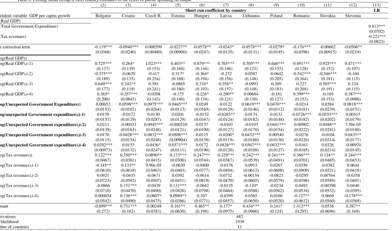
estimations of the effect of public expenditure on output (see Table 6), Table 7 reports fiscal

multipliers for each of the 11 CEEC in our sample (Table A.2a in the Appendix presents

Table 6: Pooling Mean Group (PMG) country-estimates of the effect of public spending on output

(2) (3) (4) (5) (6) (7) (8) (9) (10) (11) (12) (13)

Short run coefficient by country LR

Dependent variable: GDP per capita growth Bulgaria Croatia Czech R. Estonia Hungary Latvia Lithuania Poland Romania Slovakia Slovenia

Log(Real GDP)

Log(Total Government Expenditure) 0.813***

(0.0702)

Log(Tax revenues) -0.221***

(0.0823)

Error correction term -0.119*** -0.0940*** 0.000599 -0.0227** -0.0578** -0.0243* -0.0578*** -0.0279* -0.176*** -0.00662 -0.0508**

(0.0368) (0.0240) (0.00480) (0.00900) (0.0247) (0.0135) (0.0131) (0.0145) (0.0396) (0.00915) (0.0219) D(Log(Real GDP))

D(Log(Real GDP),t-1) 0.725*** 0.264* 1.023*** 0.403** 0.879*** 0.765*** 0.505*** 0.646*** 0.491*** 0.925*** 0.471***

(0.137) (0.139) (0.153) (0.160) (0.144) (0.146) (0.123) (0.155) (0.128) (0.152) (0.107)

D(Log(Real GDP),t-2) -0.575*** -0.0670 -0.417 0.317* -0.364* -0.232 0.0587 -0.0642 -0.542*** -0.546*** -0.160

(0.189) (0.135) (0.254) (0.188) (0.194) (0.156) (0.148) (0.205) (0.164) (0.181) (0.115)

D(Log(Real GDP),t-3) 0.640*** 0.242** 0.391 -0.0865 0.334* 0.358** -0.0993 0.209 0.227 0.505*** 0.124

(0.177) (0.119) (0.241) (0.180) (0.193) (0.157) (0.148) (0.183) (0.204) (0.191) (0.115)

D(Log(Real GDP),t-4) 0.365* -0.257*** -0.0208 -0.175 -0.226* -0.290** 0.00684 -0.181 0.399*** -0.169 0.387***

(0.200) (0.0843) (0.143) (0.140) (0.134) (0.121) (0.130) (0.127) (0.152) (0.153) (0.0986)

D(Log(Unexpected Government Expenditure)) 0.00652 0.0598*** 0.0975*** 0.0465*** 0.0249 0.0122 0.0619*** 0.0470*** -0.0214 0.0384 0.0818*** (0.0153) (0.0102) (0.0264) (0.0113) (0.0169) (0.0129) (0.0146) (0.0112) (0.0181) (0.0239) (0.0151)

D(Log(unexpected Government expenditure),t-1) 0.0159 -0.0172 0.0130 0.0201 -0.0152 -0.0285** 0.0174 0.0133 -0.0726*** -0.0553*** 0.00515 (0.0157) (0.0129) (0.0287) (0.0129) (0.0167) (0.0124) (0.0182) (0.0148) (0.0182) (0.0202) (0.0179)

D(Log(Unexpected Government expenditure),t-2) 0.0211 -0.00433 0.0945*** -0.000310 0.0137 -0.0103 -0.0103 0.0441*** 0.00902 0.0488** 7.50e-05 (0.0139) (0.0163) (0.0248) (0.0121) (0.0190) (0.0127) (0.0170) (0.0154) (0.0222) (0.0241) (0.0180)

D(Log(Unexpected Government expenditure),t-3) 0.0170 -0.0428*** 0.0832*** 0.0508*** 0.0115 -0.0200* 0.0432*** 0.00540 -0.0276 -0.0104 0.0433** (0.0115) (0.0154) (0.0248) (0.00904) (0.0158) (0.0119) (0.0160) (0.0130) (0.0226) (0.0214) (0.0177)

D(Log(Unexpected Government expenditure),t-4) 0.0292*** 0.0153 0.0436* 0.0371*** 0.0172 0.0428*** 0.0367*** 0.0432*** 0.0163 0.0326 -0.00970 (0.00973) (0.0132) (0.0247) (0.0111) (0.0190) (0.0120) (0.0109) (0.0127) (0.0185) (0.0214) (0.0145)

D(Log(Tax revenues)) 0.122*** 0.350*** 0.0890** 0.173*** 0.247*** 0.229*** 0.242*** 0.241*** 0.366*** 0.124** 0.244***

(0.0467) (0.0361) (0.0415) (0.0300) (0.0744) (0.0387) (0.0539) (0.0491) (0.0701) (0.0485) (0.0453)

D(Log(Tax revenues),t-1) -0.145** 0.133** 9.90e-05 -0.0639 -0.0400 -0.0176 0.0913 0.0267 0.0356 -0.0382 0.0644

(0.0610) (0.0618) (0.0463) (0.0403) (0.0777) (0.0494) (0.0612) (0.0608) (0.0909) (0.0521) (0.0418)

D(Log(Tax revenues),t-2) 0.0921 -0.0435 -0.0671 0.0392 -0.0614 0.0732 -0.00154 -0.0823 -0.0295 0.00764 -0.0358

(0.0723) (0.0592) (0.0507) (0.0451) (0.0818) (0.0470) (0.0605) (0.0579) (0.0596) (0.0589) (0.0401)

D(Log(Tax revenues),t-3) -0.0866 0.151*** -0.0439 0.131*** -0.0642 -0.0135 -0.110* -0.0234 0.0492 -0.00398 0.0440

(0.0710) (0.0470) (0.0490) (0.0420) (0.0798) (0.0464) (0.0588) (0.0562) (0.0534) (0.0532) (0.0395)

D(Log(Tax revenues),t-4) 0.000854 0.136*** -0.0807* 0.0989** 0.107 -0.0399 0.0365 0.0160 -0.127** 0.0669 -0.178***

(0.0542) (0.0490) (0.0475) (0.0386) (0.0771) (0.0457) (0.0650) (0.0520) (0.0612) (0.0560) (0.0369)

Constant -0.899*** 0.731*** -0.00248 0.161** 0.465** 0.177* 0.434*** 0.241* 1.412*** 0.0538 0.387**

(0.272) (0.182) (0.0383) (0.0630) (0.198) (0.0975) (0.0960) (0.124) (0.295) (0.0696) (0.169)

Observations 482

Log likelihood 1939

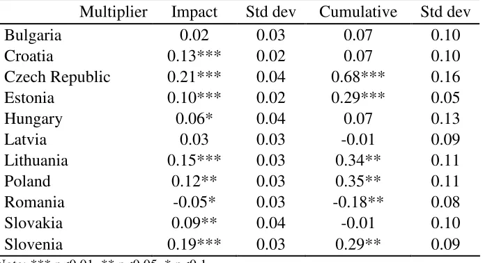
Table 7a: Fiscal multipliers by country (PMG estimator)

Multiplier Impact Std dev Cumulative Std dev

Bulgaria 0.02 0.03 0.07 0.10

Croatia 0.13*** 0.02 0.07 0.10

Czech Republic 0.21*** 0.04 0.68*** 0.16

Estonia 0.10*** 0.02 0.29*** 0.05

Hungary 0.06* 0.04 0.07 0.13

Latvia 0.03 0.03 -0.01 0.09

Lithuania 0.15*** 0.03 0.34** 0.11

Poland 0.12** 0.03 0.35** 0.11

Romania -0.05* 0.03 -0.18** 0.08

Slovakia 0.09** 0.04 -0.01 0.10

Slovenia 0.19*** 0.03 0.29** 0.09

Note: *** p<0.01, ** p<0.05, * p<0.1.

Analogous to estimations for the pooled sample, we present results for both impact

and cumulative multipliers. Let us discuss impact multipliers. First, regarding sign

differences, although most multipliers are positive, we equally reveal statistically not

significant multipliers (for example, in Bulgaria or Latvia), and even a negative impact

multiplier in Romania (albeit weakly significant). Second, we emphasize magnitude

differences across multipliers in CEEC: for example, the impact multiplier in Czech Republic

and Slovenia is roughly four times higher compared to Romania (in absolute value), and

roughly two times higher if we stick to significant positive multipliers, for example in Estonia

and Poland.

Such sign and magnitude heterogeneities equally arise if we consider the cumulated

response of GDP to fiscal shocks after four quarters. On the one hand, cumulative multipliers

are positive in most countries, and remain non significant in Bulgaria or Hungary. However,

we now find negative multipliers in three out of the eleven countries of our sample, namely

Latvia, Romania and Slovakia. On the other hand, the magnitude of cumulative multipliers is

stronger compared to impact multipliers; for example, the multiplier is around 0.3 in four

countries (Estonia, Lithuania, Poland and Slovenia), and even as high as 0.7 in Czech

Republic.

These results call for two remarks. On the one hand, recall that multipliers were

computed based on a model that assumed a common long-term path and different short-run

dynamics among CEEC. If the fact of not accounting for the long-term path (for example, like

in PVAR models) is an obvious drawback, we can illustrate the differences induced by not

which assume different long-term paths (in addition to different short-run dynamics) among

CEEC (see Table A.5 in the Appendix for MG estimated coefficients).

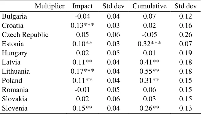
Table 7b: Fiscal multipliers by country (MG estimator)

Multiplier Impact Std dev Cumulative Std dev

Bulgaria -0.04 0.04 0.07 0.12

Croatia 0.13*** 0.03 0.02 0.16

Czech Republic 0.05 0.06 -0.05 0.26

Estonia 0.10** 0.03 0.32*** 0.07

Hungary 0.02 0.05 0.01 0.19

Latvia 0.11** 0.04 0.41** 0.18

Lithuania 0.17*** 0.04 0.55** 0.18

Poland 0.11** 0.04 0.31** 0.15

Romania -0.01 0.05 0.06 0.15

Slovakia 0.02 0.06 0.03 0.15

Slovenia 0.15** 0.04 0.26** 0.13

Note: *** p<0.01, ** p<0.05, * p<0.1.

Compared to Table 7a, Table 7b emphasizes significant difference for both impact and

cumulative multipliers. Focusing on impact multipliers, not accounting for a common

long-term path would (i) overestimate their significance in Latvia and underestimate it in Czech

Republic, Slovakia, and, to some extent, in Romania, and (ii) overestimate their size in Latvia

and underestimate it in Czech Republic and Slovakia. These differences are reinforced

regarding cumulative multipliers. For example, not accounting for a common long-term path

would (i) overestimate their significance in Latvia and underestimate it in Czech Republic,

Romania and Slovakia, and (ii) overestimate their size in Latvia and Lithuania, and

underestimate it in Czech Republic and in Romania (particularly for Romania, the estimated

coefficient would be positive, instead of significantly negative).

On the other hand, country-evidence unveils important short-run heterogeneities

across CEEC. Consistent with the standard ISLM model, we emphasize Keynesian effects of

fiscal policy both on impact and after one year, in most of CEEC in our sample. However, in

several countries we do not find significant multipliers, neither on impact (for example, in

Bulgaria and Hungary), nor cumulated after four quarters (for example, in Bulgaria and

Latvia), in line with the Ricardian Equivalence Theorem of Barro (1974). In addition, we

even find anti-Keynesian effects of fiscal policy on output, in the form of negative multipliers

(for example, in Romania on impact, and in Latvia, Romania and Slovakia cumulated after

four quarters). Thus, even if CEEC are expected to converge in the long-run towards a

common steady-state, the dynamic of their output following fiscal shocks might be quite

V. Fiscal multipliers in CEEC: Conditionality upon structural characteristics

Heterogeneities in output’s response to fiscal policy unveiled in the previous section are

probably related to economic and structural differences among CEEC. In the following, we

analyze the sensitivity of multipliers to such differences.

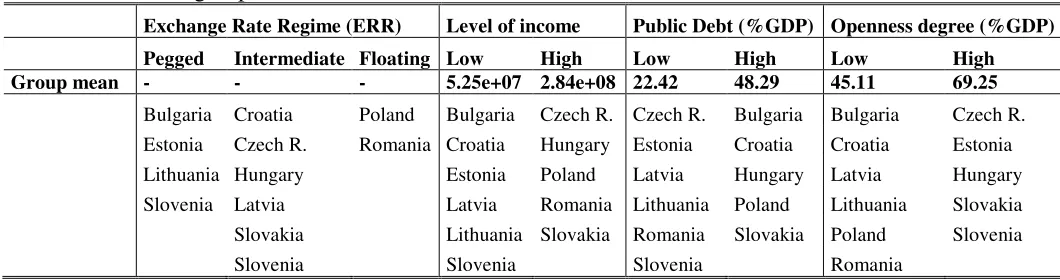
We consider four structural characteristics of CEEC. First, we seize differences in

monetary policy by considering alternatively countries with fixed (pegged), intermediate and

flexible exchange rate regime (ERR), using the classification of Ilzetzki et al. (2010) reported

in Table A.3 in the Appendix. Second, to account for the level of economic development, we

divide CEEC using the level of income (average over 1999:q1-2013:q3), into low- and

high-income CEEC, respectively. Third, we capture the fiscal stance using the public debt9 to

distinguish among low-debt CEEC (with a debt ratio of 22% of GDP on average over

1999:q1-2013:q3) and high-debt CEEC (with an average debt ratio of 48% of GDP for the

same period).10 Finally, we take into account the openness degree using the level of exports in

percentage of GDP, and, accordingly, we divide CEEC into countries with relatively low and

high openness degree, respectively. Table 8 presents the countries in each group.

Table 8: List of groups of countries based on CEEC’ structural characteristics

Exchange Rate Regime (ERR) Level of income Public Debt (%GDP) Openness degree (%GDP) Pegged Intermediate Floating Low High Low High Low High

Group mean - - - 5.25e+07 2.84e+08 22.42 48.29 45.11 69.25

Bulgaria Croatia Poland Bulgaria Czech R. Czech R. Bulgaria Bulgaria Czech R. Estonia Czech R. Romania Croatia Hungary Estonia Croatia Croatia Estonia Lithuania Hungary Estonia Poland Latvia Hungary Latvia Hungary Slovenia Latvia Latvia Romania Lithuania Poland Lithuania Slovakia Slovakia Lithuania Slovakia Romania Slovakia Poland Slovenia Slovenia Slovenia Slovenia Romania

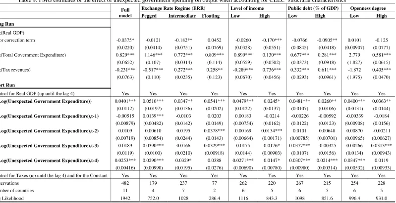
Based on Table 8, Table 9 presents the estimations of the effect of unexpected

government spending on output using the PMG estimator,11 and Table 10 reports the

associated multipliers (Table A.2b in the Appendix presents descriptive statistics for each

group of countries).

9

We use the gross consolidated debt of the central government (the same measures is used, for example, by Ilzetzki et al., 2013).

10

We split countries based on the median public debt to GDP ratio for the sample period 1999:q1-2013:q3. Considering median public debt, instead of an exogenous threshold of 60% (as suggested by the Maastricht Treaty), is justified by the fact that in our sample only Hungary presents a debt ratio above this threshold.

11

Table 9: PMG estimates of the effect of unexpected government spending on output when accounting for CEEC’ structural characteristics

Exchange Rate Regime (ERR) Level of income Public debt (% of GDP) Openness degree

Full

model Pegged Intermediate Floating Low High Low High Low High

Long Run

Log(Real GDP)

Error correction term -0.0375* -0.0121 -0.182** 0.0452 -0.0260 -0.170*** -0.0766 -0.0905** 0.0101 -0.125 (0.0220) (0.0414) (0.0751) (0.0769) (0.0328) (0.0551) (0.0845) (0.0418) (0.00907) (0.0777) Log(Total Government Expenditure) 0.829*** 1.146*** 0.772*** 0.809*** 0.899*** 0.130*** 0.677*** 0.281*** 2.779 0.581*** (0.0652) (0.107) (0.0314) (0.114) (0.0559) (0.0502) (0.0373) (0.0918) (1.827) (0.0615) Log(Tax revenues) -0.231*** -0.517*** 0.272*** 0.258** -0.289*** 0.736*** 0.332*** 0.611*** -1.872 0.405*** (0.0763) (0.110) (0.0235) (0.123) (0.0670) (0.0456) (0.0293) (0.0961) (1.975) (0.0470) Short Run

Control for Real GDP (up until the lag 4) Yes Yes Yes Yes Yes Yes Yes Yes Yes Yes D(Log(Unexpected Government Expenditure)) 0.0401*** 0.0510*** 0.0347** 0.0541*** 0.0479*** 0.0245* 0.0481*** 0.0260** 0.0400*** 0.0363**

(0.0112) (0.0197) (0.0136) (0.0202) (0.0122) (0.0137) (0.0107) (0.0106) (0.0131) (0.0144) D(Log(Unexpected Government Expenditure),t-1) -0.00515 0.0139*** -0.0103 0.0203 0.00183 -0.0214 -0.00226 -0.00592 -0.00339 -0.0184

(0.00879) (0.00482) (0.0142) (0.0149) (0.00754) (0.0162) (0.0122) (0.0123) (0.00908) (0.0156) D(Log(Unexpected Government Expenditure),t-2) 0.0109 0.00610 0.0195 0.0378*** 0.00169 0.0134*** 0.0101 0.00648 0.00870 -0.00211 (0.00719) (0.00854) (0.0244) (0.0143) (0.00664) (0.00171) (0.00785) (0.00701) (0.00965) (0.00627) D(Log(Unexpected Government Expenditure),t-3) 0.0189 0.0390*** 0.0166 0.0329*** 0.0175 0.0176* 0.0377*** -0.00325 0.00266 0.0313*** (0.0119) (0.0100) (0.0210) (0.00918) (0.0144) (0.00903) (0.0107) (0.0156) (0.0134) (0.00943) D(Log(Unexpected Government Expenditure),t-4) 0.0253*** 0.0290*** 0.0329* 0.0388 0.0271*** 0.0147* 0.0307*** 0.0214*** 0.0347*** 0.0119

(0.00416) (0.00990) (0.0195) (0.0276) (0.00690) (0.00780) (0.00980) (0.00314) (0.00532) (0.00933) Control for Taxes (up until the lag 4) and for the Constant Yes Yes Yes Yes Yes Yes Yes Yes Yes Yes

Observations 482 179 237 77 262 220 267 215 254 228

Number of countries 11 4 7 2 6 5 6 5 6 5

Log Likelihood 1942 752.0 1028 286.4 1116 843.3 1098 851.6 996.4 931.0 Note: Standard errors in brackets. *** p<0.01, ** p<0.05, * p<0.1. Total government expenditure captures the discretionary component of government spending (the residuals

Table 10: Fiscal multipliers when accounting for CEEC’ structural characteristics (PMG)

Multiplier Impact Std dev Cumulative Std dev

Full model 0.09*** 0.02 0.21** 0.07

Exchange Rate Regime

Pegged 0.11** 0.04 0.32*** 0.05

Intermediate 0.07** 0.03 0.20 0.15

Floating 0.13** 0.05 0.46*** 0.04

Level of Economic Development

Low income 0.11*** 0.02 0.22** 0.06

High income 0.05 0.03 0.11 0.07

Level of Debt-to-GDP Ratio

Low debt 0.10*** 0.02 0.28*** 0.07

High debt 0.06** 0.02 0.10 0.06

Openness Degree

Low openness 0.11*** 0.02 0.26** 0.07

High openness 0.08** 0.03 0.13 0.09

Note: *** p<0.01, ** p<0.05, * p<0.1.

Let us first focus on the type of the exchange rate regime. As shown by Table 10, the ERR

does not seem to matter for the impact response of output to changes in fiscal policy: impact

multipliers equal 0.11, 0.07 and 0.13, respectively. On the contrary, cumulative multipliers

are highly sensitive to the ERR. For example, on the one hand, the cumulated response of

output is 0.32 for pegged ERR, compared to statistically 0 (i.e. not significant) for

intermediate ERR, consistent with the Mundell-Fleming model and previous evidence of

more effective fiscal stimulus under pegged regimes in developed countries (Born et al.,

2013). On the other hand, the cumulated fiscal multiplier for floating ERR equals 0.46, and is

equally higher than for intermediate ERR, consistent yet again with evidence for developed

countries (Monacelli and Perotti, 2010, Ramey, 2011).12 These results asserting that corner

(namely, pegged and flexible) ERR perform better than intermediate ERR when it comes to

fiscal multipliers seem to suggest that the weak credibility of intermediate ERR in CEEC in

our sample reduces the efficiency of fiscal policy.

Second, using median income as cut-off, Table 10 shows that the multiplier is

sensitive to the level of economic development. Specifically, both impact and cumulative

multipliers are significant only in low-income, relative to high-income CEEC. Thus, our

findings suggest the presence of growth-effects of fiscal policies in less developed CEEC.

12

Third, to account for a potential role of the fiscal stance, we compute multipliers for

CEEC with relatively low and high debt-to-GDP ratios, respectively. Result in Table 10

display impact multipliers of 0.10 and 0.06, and cumulative multipliers of 0.28 and

statistically 0 for CEEC with low and high debt, respectively. Thus, our findings mirror the

recent literature emphasizing nonlinear effects of fiscal policy on economic growth in a

context of relatively high public debt,13 and defend sound macroeconomic environments (and

particularly, low debt) as a tool for reinforcing the efficiency of fiscal-policy-based measures

for supporting economic growth.

Finally, we use the level of exports in percentage of GDP to divide CEEC between

countries with low and high openness degree, respectively. As this was the case for the ERR,

the openness degree is not found to influence the effects of fiscal policy on impact. On the

contrary, cumulative multipliers are significant only in relatively less open CEEC (0.26,

against statistically 0 in relatively more open CEEC), consistent with the predictions of the

conventional Mundell-Fleming model.

VI. Conclusion

Despite an impressive strand of literature estimating fiscal multipliers in developed countries,

evidence for developing and emerging countries remains remarkably scarce. This paper

provides new insights into how fiscal stimulus affects the output in 11 emerging Central and

Eastern European Countries, based on a rather different methodological approach. Indeed, if

most studies draw upon VAR models, we use a Panel Vector Error Correction model, selected

for its particularly appealing features when it comes to CEEC: on the one hand, it allows

accounting for their common long-run path, supported by their integration in the E(M)U, and,

on the other hand, it permits computing different short-run dynamics in an integrated

framework that controls for their common long-run path. In addition, we pay special attention

to identifying truly exogenous shocks, through implementing an econometric procedure

together with using genuine quarterly data.

Estimations performed over the period 1999q1-2013q3 unveil the following results.

First, fiscal multipliers are positive and significant for CEEC, albeit with important

differences between impact and four-quarter cumulative multipliers. Second, country-specific

multipliers are heterogeneous across CEEC, in sign, significance, and magnitude. Third,

13

impact and cumulative fiscal multipliers are strongly sensitive to CEEC’ characteristics. In

particular, we find significant multipliers in CEEC with fixed or floating ERR, in less

developed CEEC, in the CEEC with relatively low public debt-to-GDP ratios, and in

relatively less open CEEC.

These results have important policy implications. On the one hand, our findings

suggest that a strategy for improving the growth effects for fiscal policy in small open CEEC

is to move towards extreme ERR. This is a particularly appealing finding, since some CEEC

already integrated the euro zone, and the remaining should perform structural reforms that

would allow them to join the euro zone in the future, including more fixity in their exchange

rate arrangements. On the other hand, conditionally upon a sound fiscal stance, our paper

makes the case for fiscal policies as a device for supporting economic growth in less

REFERENCES

- Afonso A., L. Agnello and D. Furceri (2010) “Fiscal policy responsiveness, persistence and

Discretion”, Public Choice, 145: 503-530.

- Agnello L., D. Furceri and R.M. Sousa (2013) “How Best Measure Discretionary Fiscal

Policy? Assessing its impact on private spending”, Economic Modelling, 34: 15-24.

- Almunia M., A. Benetrix, B. Eichengreen, K.H. O’Rourke and G. Rua (2010) “From Great

Depression to Great Credit Crisis: similarities, differences and lessons”, Economic Policy,62:

219-265.

- Banerjee A., J.J. Dolado. and R. Mestre (1998) “Error-correction mechanism tests for

cointegration in a single-equation framework”, Journal of Time Series Analysis, 19: 267-283.

- Barro R. (1974) “Are government bonds net wealth?”, Journal of Political Economy, 82:

1095-1117.

- Barro R.J. and C.J. Redlick (2009) “Macroeconomic Effects from Government Purchases

and Taxes”, NBER Working Papers no. 15369.

- Blanchard O. (1981) “Output, the Stock Market, and Interest Rates”, American Economic

Review, 71: 132-143.

- Blanchard O. (1993) “Suggestions for a New Set of Fiscal Indicators,” in H. A. A. Verbon

and F. A. A. M. van Winden, eds., The New Political Economy of Government Debt,

Amsterdam, The Netherlands: Elsevier Science Publishers.

- Blanchard O. and D. Leigh (2013) “Growth forecast errors and fiscal multipliers”, American

Economic Review, 103: 117-120.

- Blanchard O. and R. Perotti (2002) “An empirical characterization of the dynamic effects of

changes in government spending and taxes on output”, Quarterly Journal of Economics, 117:

1329-1368.

- Born B., F. Juessen and G. Muller (2013) “Exchange rate regimes and fiscal multipliers”,

Journal of Economic Dynamics & Control, 37: 446-465.

- Chahrour R., S. Schmitt-Grohé and M. Uribe (2012) “A Model-Based Evaluation Of The

Debate On The Size Of The Tax Multiplier”, AEJ: Economic Policy, 4: 28-45.

- Choi I. (2001) “Unit root tests for panel data”, Journal of International Money and Finance,

20: 249-272.

- Corsetti G., A. Meier and G. Müller (2012) “What determines government spending

multipliers?”, Economic Policy, 27: 521-565.

- Dalic M. (2013) “Cyclical properties of fiscal policy in new member states of the EU”,

Post-Communist Economies, 25: 289-308.

- Eberhardt M., A. Presbitero (2013) “This Time They Are Different: Heterogeneity and

Nonlinearity in the Relationship Between Debt and Growth”, IMF Working Paper no. 13/248.

- Egert B. (2015) “Public debt, economic growth and nonlinear effects: Myth or reality?”,

Journal of Macroeconomics, 43: 226-238.

- Fatas A. and I. Mihov (2006) “The Macroeconomic Effects of Fiscal Rules in US States”,

Journal of Public Economics, 90: 101-117.

- Fatas A. and I. Mihov (2003) “The case for restricting fiscal policy discretion”, Quarterly

Journal of Economics, 118: 1419-1447.

- Gechert S. and H. Will (2012) “Fiscal multipliers: A meta regression analysis”, IMK

Working Paper no. 97.

- Hicks J. (1937) “Mr. Keynes and the 'Classics', A Suggested Interpretation”, Econometrica,

5: 147-159.

- Ilzetzki E., E.G. Mendoza. and C.A. Végh (2013) “How Big (Small?) are Fiscal

Multipliers”, Journal of Monetary Economics, 60: 239-254.

- Ilzetzki E, C.M. Reinhart and K.S. Rogoff (2010) “Exchange Rate Arrangements Entering

- Ilzetzki E. and C. Végh (2008) “Procyclical Fiscal Policy In Developing Countries: Truth Or

Fiction?”, NBER Working Paper no. 14191.

- Im K. S., M. H. Pesaran and Y. Shin (2003) “Testing for unit roots in heterogeneous

panels”, Journal of Econometrics, 115: 53-74.

- International Institute for Labour Studies (IILS) (2011) “A review of global fiscal stimulus”,

EC-IILS Joint Discussion Paper Series no. 5.

- International Monetary Fund (IMF) (2008) World Economic Outlook, October.

- Josifidis K, J.-P. Allegret and E. Beker Pucar (2013) “Adjustment mechanisms and

exchange rate regimes in 2004 new EU members during the financial crisis”, Post-Communist

Economies, 25: 1-17.

- Keynes J. (1936) “The General Theory of Employment, Interest and Money”, Palgrave

Macmillan.

- Kourtellos, A., T. Stengos and C. Ming Tan (2014) “The effect of public debt on growth in

multiple regimes”, Journal of Macroeconomics, 38: 35-43.

- Kraay A. (2012) “How Large Is the Government Spending Multiplier? Evidence from

World Bank Lending”, Quarterly Journal of Economics, 127: 829-887.

- Kraay A. (2014) “Government Spending Multipliers in Developing Countries. Evidence

from Lending by Official Creditors”, AEJ: Macroeconomics, 6: 170-208.

- Levin A., C.-F. Lin and C.-S. J. Chu (2002) “Unit root tests in panel data: Asymptotic and

finite-sample properties”, Journal of Econometrics,108: 1-24.

- Long J. and C. Plosser (1983) “Real business cycle”, Journal of Political Economy, 91:

39-69.

- Marglin A. and P. Spiegler. (2013) “Unpacking the Multiplier: Making Sense of Recent

Assessments of Fiscal Stimulus Policy”, Social Research, 3: 819-854.

- Minea, A. and L. Mustea (2015) “A fresh look at fiscal multipliers: one size fits it all?

Evidence from the Mediterranean area”, Applied Economics, 47: 2728-2744

- Minea, A. and A. Parent (2012) “Is High Public Debt always Harmful to Economic Growth?

Reinhart and Rogoff and Some Complex Nonlinearities”, AFC Working Paper no. 2012-8.

- Monacelli T. and R. Perotti (2010) “Fiscal policy, the real exchange rate and traded goods”,

Economic Journal, 120: 437-461.

- Mooney C.Z. and R.D. Duval (1993) “Bootstrapping: A Nonparametric Approach to

Statistical Inference”, Newbury Park, CA: Sage.

- Nakamura E. and J. Steinsson (2014) “Fiscal Stimulus in a Monetary Union: Evidence from

US Regions”, American Economic Review, 104: 753-745.

- Nenovsky N. and P. Villieu (2011) “EU enlargement and monetary regimes from the

insurance model perspective”, Post-Communist Economies, 23: 433-447.

- Pedroni P. (2004). “Panel cointegration: asymptotic and finite sample properties of pooled

time series tests with an application to the PPP hypothesis”, Econometric Theory, 3: 579-625.

- Pesaran M.H., Y. Shin and R.P. Smith (1999) “Pooled mean group estimation of dynamic

heterogeneous panels”, Journal of the American Statistical Association, 94: 621-634.

- Pesaran M.H. and R.P. Smith (1995) “Estimating long-run relationships from dynamic

heterogeneous panels”, Journal of Econometrics, 68: 79-113.

- Ramey V. (2011) “Identifying government spending shocks: it’s all in the timing”,

Quarterly Journal of Economics, 126: 1-50.

- Romer C. and D. Romer (2010) “The Macroeconomic Effects of Tax Changes: Estimates

Based on a New Measure of Fiscal Shocks”, American Economic Review, 100: 763-801

- Westerlund J. (2007) “Testing for Error Correction in Panel Data”, Oxford Bulletin of

APPENDIX

(TO BE PUBLISHED EXCLUSIVELY AS ELECTRONIC SUPPLEMENTARY MATERIAL)

Table A.1a: List of countries

Bulgaria, Croatia, Czech Republic, Estonia, Hungary, Latvia, Lithuania, Poland, Romania, Slovakia, Slovenia

Table A.1b: Descriptive statistics

Variables Observations Mean Standard Dev Min Max

Real GDP 482 1.59e+08 1.78e+08 1.68e+07 8.76e+08

Government expenditure 482 6.75e+07 7.19e+07 7246924 4.21e+08

Tax revenues 482 1.91e+07 2.25e+07 1757586 1.16e+08

Real exchange rate 482 101.3819 11.21874 69.44 135.55

Central government debt (% GDP) 429 29.68998 18.11024 1 81

Export of goods & services (% GDP) 482 55.67858 16.1442 23.62175 89.89667

Table A.2a: Summary statistics of government expenditure in % of GDP (by country)

Mean Std Dev

Full model 42.79962 6.02706

Bulgaria 39.34807 7.50139

Croatia 44.42253 3.09011

Czech Republic 46.89297 3.09541

Estonia 47.13088 4.45549

Hungary 43.43218 5.52663

Latvia 44.40612 6.04969

Lithuania 41.18482 4.95491

Poland 38.35802 5.01909

Romania 39.54567 5.12169

Slovakia 44.36725 7.31942

Slovenia 42.85272 2.58801

Table A.2b: Summary statistics of government expenditure in % of GDP (by category)

Mean Std Dev

Full model 42.79962 6.02706

Pegged regime 42.82518 5.972292

Intermediate regime 45.07149 5.150866

Floating regime 39.68591 4.971359

Low income 42.77994 5.701126

High Income 42.82263 6.395615

Low Debt 43.80545 5.278542

High Debt 42.79962 6.02706

Low Openness 40.65295 5.876038

Table A.3: CEEC’ ERR classification based on Ilzetzki, Reinhart and Rogoff (2010)

Code Fine classification Coarse classification Countries 1 No separate legal tender Bulgaria, Estonia 2 Pre announced peg or currency board Pegged Lithuania, Slovenia

4 De facto Peg

8 De facto crawling band that is narrowed than or equal to+/-2% Croatia, Czech Republic 9 Pre announced crawling band that is wider than or equal to +/-2% Hungary, Latvia 10 De facto crawling band that is narrower than or equal to +/-5% Intermediate Slovakia 11 Moving band that is narrower than or equal to +/-2% Slovenia

(i.e., allows for both appreciation and depreciation over time)

12 Managed floating _{Floating Poland, Romania} 14 Freely falling

Table A.4: PMG estimates of the effect of unexpected government spending on output when accounting for CEEC’ structural characteristics (full Table 9)

Exchange Rate Regime (ERR) Level of income Public debt (% of GDP) Openness degree

Full

model Pegged Intermediate Floating Low High Low High Low High

Long Run

Log(Real GDP)

Error correction term -0.0375* -0.0121 -0.182** 0.0452 -0.0260 -0.170*** -0.0766 -0.0905** 0.0101 -0.125 (0.0220) (0.0414) (0.0751) (0.0769) (0.0328) (0.0551) (0.0845) (0.0418) (0.00907) (0.0777) Log(Total Government Expenditure) 0.829*** 1.146*** 0.772*** 0.809*** 0.899*** 0.130*** 0.677*** 0.281*** 2.779 0.581***

(0.0652) (0.107) (0.0314) (0.114) (0.0559) (0.0502) (0.0373) (0.0918) (1.827) (0.0615) Log(Tax revenues) -0.231*** -0.517*** 0.272*** 0.258** -0.289*** 0.736*** 0.332*** 0.611*** -1.872 0.405***

(0.0763) (0.110) (0.0235) (0.123) (0.0670) (0.0456) (0.0293) (0.0961) (1.975) (0.0470) Short Run

D(Log(Real GDP))

D(Log(Real GDP),t-1) 0.626*** 0.506*** 0.614*** 0.603*** 0.524*** 0.751*** 0.619*** 0.628*** 0.668*** 0.691*** (0.0701) (0.0671) (0.0859) (0.0298) (0.0736) (0.104) (0.0685) (0.123) (0.0426) (0.0978) D(Log(Real GDP),t-2) -0.183* -0.0701 -0.217** -0.0848 -0.0811 -0.228 -0.114 -0.248 -0.179 -0.169

(0.0962) (0.207) (0.0924) (0.341) (0.128) (0.147) (0.128) (0.202) (0.180) (0.132) D(Log(Real GDP),t-3) 0.216*** 0.0873 0.306*** 0.179 0.148 0.296*** 0.136* 0.430*** 0.310*** 0.174** (0.0681) (0.161) (0.0762) (0.140) (0.113) (0.0360) (0.0807) (0.103) (0.108) (0.0880) D(Log(Real GDP),t-4) -0.00700 0.162 -0.0195 0.221 0.0290 0.0589 0.144 -0.125** 0.00320 0.0446

(0.0781) (0.168) (0.160) (0.381) (0.132) (0.102) (0.124) (0.0511) (0.134) (0.108) D(Log(Unexpected Government Expenditure)) 0.0401*** 0.0510*** 0.0347** 0.0541*** 0.0479*** 0.0245* 0.0481*** 0.0260** 0.0400*** 0.0363**