Munich Personal RePEc Archive
A Nonparametric Option Pricing Model
Using Higher Moments
Cayton, Peter Julian and Ho, Kin-Yip
School of Statistics, University of the Philippines Diliman, Research
School of Finance, Actuarial Studies, and Applied Statistics, College
of Business and Economics, The Australian National University
April 2015
Online at
https://mpra.ub.uni-muenchen.de/79134/
Moments
Peter Julian Caytona
and Kin-Yip Hob
a
Research School of Finance, Actuarial Studies, and Applied Statistics, College of Business and Economics, The Australian National University, and School of Statistics, University of the Philippines Diliman b
Research School of Finance, Actuarial Studies, and Applied Statistics, College of Business and Economics, The Australian National University
Email: [email protected]
Abstract:A nonparametric pricing model of European call options that includes non-Gaussian characteristics of skewness and kurtosis is proposed based on the cubic market capital asset pricing model. It is an equilibrium pricing model but risk-neutral valuation can be introduced through return data transformation. The model complies with the put-call parity principle of Eurpoean option pricing theory. The properties of the model are studied through simulation methods and compared with the Black-Scholes model. Simulation scenarios include cases on nonnormality in skewness and kurtosis, nonconstant variance, moneyness, contract duration, and interest rate levels. The proposed model can have negative prices in cases of out-of-money options and in simulation cases that are different from real-market situations, but the frequency of negative prices is reduced when risk-neutral valuation is implemented. The model is more adaptive and more conservative in pricing options compared to the Black-Scholes model when nonnormalities exist in the returns data.
P. J. Cayton and K. Y. Ho, A nonparametric option pricing model using higher moments
1 INTRODUCTION
The paper proposes a nonparametric European call option pricing model that accounts for higher-moment features of the underlying asset returns data. This model extends the technology developed by Chen and Palmon (2005) in which the capital asset pricing model [CAPM] of Sharpe (1964) and Fama (1968) was used. The extension of the model used is the Cubic Market Model of Neslihanoglu (2014). This model complies with the Four-Moment CAPM model by Fang and Lai (1997) and Dittmar (2002) which incorporates non-Gaussian information such as skewness and kurtosis. The derived option pricing model complies with the put-call parity principle of option pricing modeling of Stoll (1969). The proposed model is based on a equilibrium asset pricing principle similar to Chen and Palmon (2005) but risk-neutral valuation of Cox and Ross (1976) can also be done by data transformation that will preserve other distribution characteristics. The properties of the proposed model is studied and compared with the Black and Scholes (1973) model through simulations by changing the assumptions on moneyness, interest rate, duration, and return distribution characteristics in terms of variance, skewness, and kurtosis.
2 DERIVATION OF THEOPTIONPRICINGMODEL
Using the cubic market model as described in Neslihanoglu (2014), its terms are substituted similar to Chen and Palmon (2005). LettandT as fractions of time in a year andT > t,Ct,T ,K as the call price at timet
with time-to-maturityT−tand strike priceK,K∗ = K
St,Rf,t,T = (1 +rA)
T−t=1 plus the unannualized
rate of return of a risk-free asset from timettoT whererAis the annual effective rate of the risk-free asset,
and{Rt,T ,1, . . . , Rt,T ,n}whereRt,T ,i = Si
Si−N(T−t) is the returns data withN is the number of time periods
in a year of which the data was disaggregated; for exampleN = 252for trading days in a year for daily data. The estimated call option priceCˆt,T ,K= ˆCt,T ,K∗ ×St, whereCˆt,T ,K∗ is equal to
ˆ
C∗
t,T ,K = 1
Rf,t,T ×
n
ˆ
Et[max{Rt,T −K∗}]−αˆ∗1,t,T ,K
h
ˆ
Et(Rt,T)−Rf,t,T
i
−αˆ∗
2,t,T ,KEˆt
h
(Rt,T−Rf,t,T)
2i
−αˆ∗
3,t,T ,KEˆt
h
(Rt,T −Rf,t,T)
3io
(1)
The values ofαˆ∗
1,t,T ,K,αˆ∗2,t,T ,K, andαˆ∗3,t,T ,K are solutions to the system of linear equations,
ˆ
β∗
t,T ,K= ˆα∗1,t,T ,K+ ˆα∗2,t,T ,K
ˆ
Covt
h
(Rt,T −Rf,t,T)
2
, Rt,T
i
ˆ
V ar(Rt,T)
+ ˆα∗
3,t,T ,K
ˆ
Covt
h
(Rt,T −Rf,t,T)
3
Rt,T
i
ˆ
V art(Rt,T)
(2)
ˆ
γ∗
t,T ,K= ˆα∗1,t,T ,K+ ˆα∗2,t,T ,K
ˆ
Coskewt
h
(Rt,T −Rf,t,T)
2
, Rt,T
i
ˆ
µ3t(Rt,T)
+ ˆα∗
3,t,T ,K
ˆ
Coskewt
h
(Rt,T −Rf,t,T)
3
, Rt,T
i
ˆ
µ3t(Rt,T)
(3)
ˆ
δ∗
t,T ,K= ˆα∗1,t,T ,K+ ˆα∗2,t,T ,K ˆ
Cokurtt
h
(Rt,T −Rf,t,T)
2
, Rt,T
i
ˆ
µ4t(Rt,T)
+ ˆα∗
3,t,T ,K ˆ
Cokurtt
h
(Rt,T −Rf,t,T)
3
, Rt,T
i
ˆ
µ4t(Rt,T)
(4)
ˆ
β∗
t,T ,K= ˆ
Covt(max{Rt,T −K∗}, Rt,T) ˆ
Vt(Rt,T)
(5)
ˆ
γ∗
t,T ,K= ˆ
Coskewt(max{Rt,T −K∗}, Rt,T) ˆ
µ3t(Rt,T)
(6)
ˆ
δ∗
t,T ,K= ˆ
Cokurtt(max{Rt,T −K∗}, Rt,T) ˆ
µ4t(Rt,T)
(7)
The hats in the terms mean estimating the quantities using method-of-moments. The proposed pricing model complies with the put-call parity property of Stoll (1969). Using the current formula, it assumes that the historical mean and the standard deviation of data will persist in future price movements. Adjusting for desired mean and variance assumptions on the asset returns,µˇt,T ,iandσˇ
2
done by letting Rˇt,T ,i =
ˇ
σt,T ,i
sRt,T,i
Rt,T ,i−R¯t,T+ ˇµt,T ,i. The transformation maintains the shape of the
distribution of returns; the historical skewness and kurtosis of the data is assumed to persist in the future. Transformation to risk-neutral valuation of options can be done by letting the model fulfill the martingale condition of Cox and Ross (1976), by setting µˇt,T ,i = Rf,t,T. Special cases of the pricing model can be
generated by setting conditions on some parameters. Lettingα∗
2,t,T ,K = α∗3,t,T ,K = 0will produce the call
option price estimator similar in concept to Chen and Palmon (2005), denoted asCˆCP
t,T ,K; lettingα∗3,t,T ,K = 0
will produce the quadratic market model call option price estimator Cˆt,T ,KQM M, which is based on Kraus and Litzenberger (1976) and Barone-Adesi (1985); while the general case, the cubic market model estimator which is based on Neslihanoglu (2014), will be denoted asCˆCM M
t,T ,K . Special notations are used for denoting models
described in the paper. If a model facilitates risk-neutral valuations, theRN superscript is added. For example,
ˆ
CCM M.RN
t,T ,K implies the cubic pricing model has been adjusted for risk-neutral vaulation. The asterisk on the
pricing model notation indicates that the underlying-adjusted pricing formula is used, meaning that the pricing formula is divided by the underlying priceSt. As example, the notationCˆt,T ,K∗CM M means that the cubic pricing
model has been divided by the underlying price.
3 SIMULATIONSTUDY
The properties of the new pricing model and its special cases will be studied and compared with the Black and Scholes (1973) pricing model for European call options, which isCˆBS
t,T ,K=St×Cˆt,T ,K∗BS where
ˆ
C∗BS t,T ,K = Φ
−lnK∗
t +
r+ˆσ2 2
(T−t) ˆ
σ√T−t
−Kt∗exp{−r(T −t)}Φ
−lnK∗
t +
r−σˆ2 2
(T−t) ˆ
σ√T−t
(8)
andr= ln(1 +rA)is the continuous compounding interest rate of the risk-free asset, whererAis the annual
effective interest rate of the asset. The termΦ(•)is the cumulative density function of the standard normal distribution. The estimator ofσin the Black-Scholes model will be based on Gross (2006):
ˆ σ= v u u t 1
n−1
n
X
i=1
(ut,T ,i−u¯t,T)
2
√
T−t (9)
The termsut,T ,i = lnRt,T ,iis the log-returns at timeiwith duration of accumulationT −tandu¯t,T is the
mean of these log-returns. The pricing models that will be compared through simulation studies areCˆ∗BS
t,T ,K, ˆ
C∗CP
t,T ,K,Cˆ∗ CP,RN t,T ,K ,Cˆ∗
QM M t,T ,K ,Cˆ∗
QM M,RN
t,T ,K ,Cˆt,T ,K∗CM M, andCˆ∗
CM M,RN
t,T ,K . The scenarios for the simulation will
be a combination of cases from different elements of the pricing model formulas: (a) interest rate of the risk-free assetrA, (b) moneynessKt∗, (c) duration of the contractT −t, (d) variance structure of the log-returns,
(e) skewness of log-returns, and (f) kurtosis of log-returns. Each scenario will consist of 100 simulated return series data, with each series data having 1260 return periods, equivalent to five-year’s worth of data.For the risk-free interest rate, three cases are assumed: the 4-week US Treasury Bills secondary market interest rate for the low rate case, the 3-year US Treasury Bond interest rate for the middle rate case, and the 20-year Treasury Bond interest rate for the high rate case. The rates used are based on the of Governors of the Federal Reserve System (2015) for the date of 31 March 2015. These rates are, respectively,0.05%p.a.,0.89%p.a. compounded semiannually, and2.31%p.a. compounded semiannually. For moneyness, the termK∗
t is varied
to five values as cases: K∗
t = 0.90 represents the case of11.11% in-the-money for the call option,0.95
represents5.26%in-the-money,1.00represents at-the-money,1.05represents4.76%out-the-money, and1.10
P. J. Cayton and K. Y. Ho, A nonparametric option pricing model using higher moments
GARCH(1,1) model is defined by Bollerslev (1986):
ut,T ,i=µt,T +ǫt,T ,i, ǫt,T ,i∼ 0, σ
2
t,T ,i
σ2
t,T ,i=ωt,T +φ1,t,Tǫ 2
t,T ,i−1+φ2,t,Tσ 2
t,T ,i−1 (10)
The GARCH(1,1) model makes the individual return variances σ2
t,T ,i of log-returns fluctuate through time
given that the unconditional historical variance of the data still is a finite constant value. The valueµt,T for
simulations will be the mean as estimated from the S&P 500 data and will only change with respect to the contract duration and the variance model of the case assumed. The statementǫt,T ,i ∼ 0, σt,T ,i2
means that the distribution will be generated from a standardized distribution that will have zero mean. The standardized distribution depends on the value of skewness and kurtosis. For the constant variance case,φ1,t,T =φ2,t,T = 0
is set. Table 1 shows the values of the parameters for different cases. The estimates ofµt,T andωt,T for
Duration Constant Variance GARCH(1,1)
µt,T ωt,T µt,T ωt,T φ1,t,T φ2,t,T
[image:5.595.160.449.236.281.2]21-day 0.01034198 0.001467624 0.021169 0.000118 0.893725 0.029669 63-day 0.03072180 0.003206283 0.043351 0.000069 0.776531 0.222469 126-day 0.06242610 0.005116157 0.073590 0.000088 0.972670 0.026330
Table 1: Parameter Values for Variance Cases
the constant variance are the corresponding method-of-moments estimates, while the GARCH(1,1) model estimates are based on quasi-maximum likelihood estimation on the S&P 500 data ending at 13 February 2015 with a span of 5 years. About skewness, three cases are assumed: negative or skewed to the left,
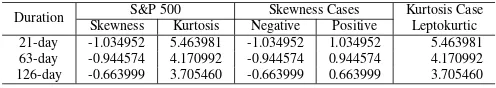
Duration S&P 500 Skewness Cases Kurtosis Case Skewness Kurtosis Negative Positive Leptokurtic 21-day -1.034952 5.463981 -1.034952 1.034952 5.463981 63-day -0.944574 4.170992 -0.944574 0.944574 4.170992 126-day -0.663999 3.705460 -0.663999 0.663999 3.705460
Table 2: Parameter Values for Skewness and Kurtosis Cases
zero or symmetric, and positive or skewed to the right. The value of skewness is based on the S&P 500 data and would be different for every contract duration considered. Table 2 shows the value of skewness per case and duration, based on the skewness of the S&P 500 data. With respect to kurtosis, two cases are considered: the mesokurtic case, where kurtosis is equal to 3, and the leptokurtic or heavy-tails case, where the kurtosis is based on the S&P 500 data and returns based on contract duration. Table 2 contains the values of kurtosis that will be used for the simulation studies. Since nonnormal features will be part of the cases of the simulations, when nonzero skewness or nonnormal kurtosis is the case, then the Johnson family of distributions Johnson (1949) is used to generate the simulated returns data. The Johnson family of distributions has the following cumulative distribution formulaF(x) = Φ{η+ζ×g[(x−ξ)/λ]}The functiong(•)is a function that determines the type of distribution used for generating returns. Ifg(z) =z, then the Johnson distribution type is the normal or Gaussian distribution, denoted as SN. Ifg(z) = ln(z), then the Johnson distribution type is the lognormal distribution, marked as SL. The Johnson SU or unbounded distribution type is generated by letting g(z) = sinh−1
z, the inverse hyperbolic sine function, and the bounded distribution or SB type is by letting g(z) = ln z
1−z
[image:5.595.180.428.388.432.2]
Duration Combination of Cases Johnson Family
Skewness Kurtosis Type ξ λ η ζ
21-day Negative Mesokurtic SB -2.852114 3.876390 -0.856400 0.534582 21-day Negative Leptokurtic SU 1.609838 1.484898 2.050504 2.345450
21-day Zero Mesokurtic SN 0.000000 1.000000 0.000000 1.000000
21-day Zero Leptokurtic SU 0.000000 1.422798 0.000000 1.706085 21-day Positive Mesokurtic SB -1.024276 3.876390 0.856400 0.534582 21-day Positive Leptokurtic SU -1.609837 1.484898 -2.050504 2.345450 63-day Negative Mesokurtic SB -3.155855 4.353278 -0.908420 0.673890 63-day Negative Leptokurtic SB -10.935399 13.237225 -3.086450 1.873181
63-day Zero Mesokurtic SN 0.000000 1.000000 0.000000 1.000000
63-day Zero Leptokurtic SU 0.000000 1.964320 0.000000 2.188413 63-day Positive Mesokurtic SB -1.197423 4.353278 0.908420 0.673890 63-day Positive Leptokurtic SB -2.301826 13.237225 3.086450 1.873181 126-day Negative Mesokurtic SB -4.559566 6.540898 -1.183885 1.251032 126-day Negative Leptokurtic SL* 4.589575 -1.000000 -6.967738 4.643311
126-day Zero Mesokurtic SN 0.000000 1.000000 0.000000 1.000000
[image:6.595.147.463.62.224.2]126-day Zero Leptokurtic SU 0.000000 2.476362 0.000000 2.661838 126-day Positive Mesokurtic SB -1.981333 6.540898 1.183885 1.251032 126-day Positive Leptokurtic SL* -4.589575 1.000000 -6.967738 4.643311
Table 3: Johnson Dsitribution Parameter Values and Types for Simulations
An asterisk beside the SL indicates that SB estimation would not converge, so the lognormal distribution was used to approximate the nonnormal features. Overall, there are 540 scenarios in the simulation experiments. These simulation results will be evaluated based comparisons of valuations from different cases. The average price value will be reported in tables. From the simulations, negative option prices were observed from some cases in the proposed pricing model. To investigate this, the percentage of negative option prices per case in each model is computed.
[image:6.595.87.522.418.527.2]4 RESULTS ANDDISCUSSION
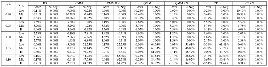
Table 4 contains the summary of simulation results considering the moneyness and interest rate, ignoring other simulation scenarios.
K∗ rA BS CMM CMM.RN QMM QMM.RN CP CP.RN
Aver. % Neg. Aver. % Neg. Aver. % Neg. Aver. % Neg. Aver. % Neg. Aver. % Neg. Aver. % Neg.
0.90
Low 10.11% 0.00% 9.09% 0.22% 9.96% 0.06% 10.28% 0.00% 9.92% 0.00% 10.24% 0.00% 10.19% 0.00% Mid 10.31% 0.00% 10.28% 0.44% 10.16% 0.00% 10.46% 0.00% 10.13% 0.00% 10.44% 0.00% 10.39% 0.00% Hi 10.64% 0.00% 10.66% 0.22% 10.48% 0.08% 10.77% 0.00% 10.48% 0.00% 10.77% 0.00% 10.72% 0.00%
0.95
Low 5.59% 0.00% 5.60% 1.08% 5.19% 0.08% 5.63% 0.00% 5.04% 0.00% 5.58% 0.00% 5.59% 0.00% Mid 5.76% 0.00% 5.29% 1.22% 5.32% 0.06% 5.79% 0.00% 5.24% 0.00% 5.78% 0.00% 5.78% 0.00% Hi 6.06% 0.00% 5.66% 0.92% 3.76% 0.08% 6.07% 0.00% 5.58% 0.00% 6.11% 0.00% 6.08% 0.00%
1.00
Low 2.25% 0.00% 0.10% 7.81% 1.42% 0.31% 1.80% 0.00% 1.25% 0.00% 1.69% 0.00% 2.07% 0.00% Mid 2.36% 0.00% 2.66% 6.86% 1.52% 0.39% 1.90% 0.00% 1.36% 0.00% 1.87% 0.00% 2.18% 0.00% Hi 2.57% 0.00% 1.93% 6.89% 1.66% 0.31% 2.09% 0.00% 1.58% 0.00% 2.17% 0.00% 2.38% 0.00%
1.05
Low 0.66% 0.00% -3.09% 52.25% 0.17% 22.75% 0.01% 64.03% 0.03% 51.61% -0.34% 61.81% 0.69% 0.00% Mid 0.71% 0.00% 0.22% 50.14% 0.22% 20.11% 0.03% 63.33% 0.06% 46.03% -0.22% 53.78% 0.73% 0.00% Hi 0.80% 0.00% 0.43% 49.22% 0.21% 16.83% 0.08% 61.03% 0.11% 36.47% 0.00% 43.72% 0.80% 0.00%
1.10
Low 0.16% 0.00% -0.04% 44.78% -0.06% 65.36% -0.22% 80.64% -0.14% 86.67% -0.73% 82.53% 0.27% 0.00% Mid 0.17% 0.00% -0.01% 47.53% -0.04% 62.78% -0.24% 84.47% -0.14% 86.92% -0.65% 80.44% 0.28% 0.00% Hi 0.21% 0.00% -2.67% 48.53% 0.00% 61.22% -0.26% 88.72% -0.13% 84.25% -0.51% 71.64% 0.31% 0.00%
Table 4: Average Call Prices in Percent of Underlying Asset Price and Percentage of Negative Call Prices by Model, Interest Rate, and Moneyness Cases
From the table, negative prices may tend to occur for the CMM, CMM.RN, QMM, QMM.RN, and CP models, and these occurrences increase as the K∗ increases. Risk-neutral valuated models are less likely to have
negative prices, and the CP.RN and BS models, which are risk-neutral models, cannot have negative prices. The most frequent occurrences of negative prices tend to occur at out-of-money situations. With respect to average call option prices, CMM, CMM.RN, and QMM.RN tend to have lower prices compared to the BS model for in-the-money cases. QMM, CP, and CP.RN tend to have higher price valuations compared to the BS for in-the-money cases. For at-the-money cases, all proposed models tend to have lower valuations compared to the BS model, with the CP.RN model being the closest model to the BS valuation. It is notable that the CP.RN model tends to have higher or equal valuations to the BS model, except for at-the-money cases.
P. J. Cayton and K. Y. Ho, A nonparametric option pricing model using higher moments
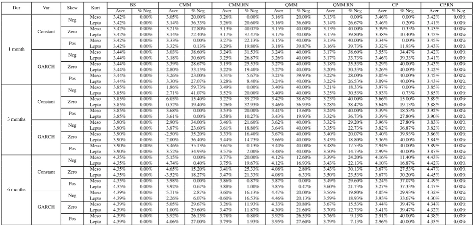
Dur Var Skew Kurt Aver. BS% Neg. Aver.CMM% Neg. Aver.CMM.RN% Neg. Aver.QMM% Neg. Aver.QMM.RN% Neg. Aver. CP% Neg. Aver.CP.RN% Neg.
1 month Constant
Neg Meso 3.42% 0.00% 3.05% 20.00% 3.26% 0.00% 3.16% 20.00% 3.13% 0.00% 3.46% 0.00% 3.42% 0.00% Lepto 3.42% 0.00% 3.14% 36.33% 3.26% 20.60% 3.16% 36.60% 3.14% 26.67% 3.46% 0.20% 3.41% 0.00%
Zero Meso 3.42% 0.00% 3.21% 12.80% 3.13% 40.07% 3.15% 40.00% 3.13% 40.00% 3.39% 0.33% 3.43% 0.00% Lepto 3.42% 0.00% 3.14% 22.40% 3.17% 37.47% 3.17% 40.00% 3.15% 39.80% 3.38% 10.40% 3.42% 0.00%
Pos Meso 3.42% 0.00% 3.33% 0.00% 3.27% 22.13% 3.15% 40.00% 3.13% 40.00% 3.34% 0.00% 3.45% 0.00% Lepto 3.42% 0.00% 3.32% 0.13% 3.29% 19.80% 3.18% 39.87% 3.16% 39.73% 3.32% 11.93% 3.43% 0.00%
GARCH
Neg MesoLepto 3.44%3.44% 0.00%0.00% 3.03%3.18% 38.60%30.60% 3.24%3.25% 31.53%26.87% 3.26%3.24% 40.00%40.00% 3.17%3.17% 33.73%38.60% 3.46%3.55% 39.33%34.47% 3.41%3.42% 0.00%0.00%
Zero MesoLepto 3.44%3.44% 0.00%0.00% 3.39%2.80% 28.67%33.13% 3.19%3.22% 25.53%19.40% 3.27%3.27% 40.00%40.00% 3.20%3.18% 30.33%35.53% 3.26%3.29% 40.00%40.00% 3.42%3.43% 0.00%0.00%
Pos MesoLepto 3.44%3.44% 0.00%0.00% 3.26%3.30% 23.00%27.07% 3.31%3.28% 5.67%8.40% 3.24%3.21% 40.00%39.93% 3.22%3.22% 26.53%28.00% 3.09%3.05% 40.00%40.00% 3.43%3.45% 0.00%0.00%
3 months Constant
Neg MesoLepto 3.85%3.85% 0.00%0.00% 1.86%2.71% 59.73%41.07% 3.49%3.52% 20.00%0.00% 3.40%3.40% 40.00%40.00% 3.25%3.21% 30.53%18.33% 3.93%3.97% 0.73%0.00% 3.85%3.85% 0.00%0.00%
Zero MesoLepto 3.85%3.85% 0.00%0.00% 6.03%0.52% 15.40%19.40% 3.22%3.26% 39.27%32.93% 3.46%3.42% 36.93%38.67% 3.28%3.23% 38.47%40.00% 3.64%3.66% 19.13%15.00% 3.88%3.89% 0.00%0.00%
Pos MesoLepto 3.85%3.85% 0.00%0.00% 3.68%3.61% 0.00%0.00% 3.53%3.58% 20.00%10.27% 3.43%3.41% 19.93%13.60% 3.32%3.24% 36.73%40.00% 3.39%3.39% 27.80%18.53% 3.90%3.92% 0.00%0.00%
GARCH
Neg MesoLepto 3.90%3.90% 0.00%0.00% 2.90%3.87% 34.00%23.60% 3.46%3.61% 21.60%18.80% 3.64%3.62% 40.00%40.00% 3.35%3.32% 22.73%29.20% 3.82%3.96% 36.87%27.80% 3.82%3.83% 0.00%0.00%
Zero MesoLepto 3.90%3.90% 0.00%0.00% -2.50%2.00% 35.20%36.40% 3.33%3.44% 16.40%14.73% 3.66%3.67% 40.00%40.00% 3.43%3.40% 18.80%20.07% 3.36%3.40% 40.00%39.93% 3.84%3.86% 0.00%0.00%
Pos Meso 3.90% 0.00% 3.46% 35.13% 3.61% 0.13% 3.44% 40.00% 3.48% 17.53% 2.94% 40.00% 3.89% 0.00% Lepto 3.90% 0.00% 3.52% 34.93% 3.57% 2.00% 3.48% 40.00% 3.50% 14.73% 2.99% 40.00% 3.87% 0.00%
6 months Constant
Neg Meso 4.35% 0.00% 5.15% 0.00% 3.77% 20.00% 4.12% 12.60% 3.39% 24.20% 4.16% 11.40% 4.43% 0.00% Lepto 4.35% 0.00% 4.74% 0.40% 3.75% 19.67% 4.12% 16.93% 3.43% 22.13% 4.10% 16.87% 4.42% 0.00%
Zero Meso 4.35% 0.00% 4.65% 15.20% 3.41% 25.33% 4.08% 2.80% 3.43% 30.13% 3.67% 27.53% 4.47% 0.00% Lepto 4.35% 0.00% -3.52% 18.27% 3.47% 21.33% 4.08% 6.33% 3.50% 23.53% 3.67% 30.20% 4.45% 0.00%
Pos Meso 4.35% 0.00% 3.98% 0.00% 3.86% 0.87% 3.87% 0.00% 3.49% 29.60% 3.24% 37.07% 4.49% 0.00% Lepto 4.35% 0.00% 3.92% 0.67% 3.88% 1.00% 3.85% 0.47% 3.60% 21.73% 3.27% 37.33% 4.47% 0.00%
GARCH
Neg Meso 4.39% 0.00% 5.71% 2.87% 3.60% 16.13% 4.47% 20.00% 3.56% 19.80% 4.05% 29.93% 4.32% 0.00% Lepto 4.39% 0.00% 2.26% 6.07% -0.60% 16.53% 4.46% 20.13% 3.59% 18.93% 3.93% 33.67% 4.30% 0.00%
Zero Meso 4.39% 0.00% 5.05% 29.67% 3.26% 11.93% 4.33% 20.80% 3.67% 15.53% 3.44% 39.47% 4.34% 0.00% Lepto 4.39% 0.00% 1.00% 29.60% 3.47% 11.87% 4.30% 21.60% 3.70% 12.73% 3.41% 39.47% 4.32% 0.00%
[image:7.595.85.570.61.291.2]Pos Meso 4.39% 0.00% 3.92% 26.13% 3.78% 0.80% 3.92% 26.53% 3.76% 9.13% 2.91% 40.00% 4.38% 0.00% Lepto 4.39% 0.00% 4.06% 27.00% 3.79% 1.93% 3.95% 27.60% 3.79% 7.13% 2.96% 40.00% 4.35% 0.00%
Table 5: Average Call Price and Percentage of Negative Call Prices by Model, Duration, Variance Structure, Skewness, and Kurtosis Cases
negative option prices tends to be spread to almost all cases but of differing frequency. With respect to average call price values, the proposed models except CP.RN tend to be more conservative than BS in the sense that they tend value options with lower prices compared to the BS over most cases. The CP.RN model tends to give higher valuations in cases of constant variance compared to the BS model, and would be more conservative for the GARCH variances cases compared to the BS. Highlighting the real-data cases of GARCH variance, negative skewness, and leptokurtosis for all durations, the BS model tends to value call options higher than the proposed models. The longer the duration, the higher the valuations tend to be except for the CMM and CMM.RN which tend to exhibit nonlinearities on the pattern of the averages. It is notable that the whether nonnormal features are evident or not, the BS model tends to have similar values up to the second decimal of the percentage, and would only differ with respect to duration and variance structure. For the proposed models, skewness and kurtosis tend to change the option price at differing magnitudes. Overall, for five of the proposed models, negative prices are possible because: (1) the models are not based on a no-arbitrage pricing principle, but on equilibrium asset pricing models such as the CAPM, which Chen and Palmon (2005) used, and its extensions, where negative prices tend to be possible, indicating possible arbitrage gains, based on Jarrow and Madan (1997), and (2) the nature of their formula, which involves differences between quantities. Negative quantities would imply largeα∗
i,t,T ,K, which may mean large systematic variance, skewness, or kurtosis. This
implies that these large risks cannot be eliminated or reduced.
5 CONCLUSION
6 ACKNOWLEDGEMENTS
The authors would like to thank the University of the Philippines for the foreign doctoral fellowship support for the first author and the Australian National University for support through employment of first author as research assistant to compile this paper.
REFERENCES
Barone-Adesi, G. (1985, Sep.). Arbitrage equilibrium with skewed asset returns. The Journal of Financial and Quantitative Analysis 20(3), 299–313.
Black, F. and M. Scholes (1973, May-Jun). The pricing of options and corporate liabilities.Journal of Political Economy 81(3), 637–654.
Bollerslev, T. (1986). Generalized autoregressive conditional heteroscedasticity. Journal of Econometrics 31, 307–327.
Chen, R.-R. and O. Palmon (2005). A non-parametric option pricing model: Theory and empirical evidence.
Review of Quantitative Finance and Accounting 24, 115–134.
Cox, J. C. and S. A. Ross (1976). The valuation of options for alternative stochastic processes. Journal of Financial Economics 3, 145–166.
Dittmar, R. F. (2002, February). Nonlinear pricing kernels, kurtosis preference, and evidence from the cross section of equity returns.The Journal of Finance 57(1), 369–403.
Fama, E. F. (1968, March). Risk, return and equilibrium: Some clarifying comments. The Journal of Fi-nance 23(1), 29–40.
Fang, H. and T.-Y. Lai (1997, May). Co-kurtosis and capital asset pricing. The Financial Review 32(2), 293–307.
Gross, P. (2006). Parameter estimation for black-scholes equation. Technical report, Department of Mathe-matics, The University of Arizona.
Hill, I. D., R. Hill, and R. L. Holder (1976). Algorithm as 99: Fitting johnson curves by moments. Journal of the Royal Statistical Society. Series C (Applied Statistics) 25(2), 180–189.
Jarrow, R. A. and D. B. Madan (1997). Is mean-variance analysis vacuous: Or was beta still born? European Finance Review 1, 15–30.
Johnson, N. L. (1949, Jun.). Systems of frequency curves generated by methods of translation.
Biometrika 36(1/2), 149–176.
Kraus, A. and R. H. Litzenberger (1976, Sep.). Skewness preference and the valuation of risk assets. The Journal of Finance 31(1), 1085–1100.
Neslihanoglu, S. (2014).Validating and Extending the Two-Moment Capital Asset Pricing Model for Financial Time Series. Ph. D. thesis, School of Mathematics and Statistics, College of Science and Engineering, University of Glasgow.
of Governors of the Federal Reserve System, B. (2015, April). Selected interest rates (daily) - h.15. http://www.federalreserve.gov/releases/h15/data.htm. Website accessed last 7 April 2015.
Sharpe, W. F. (1964, September). Capital asset prices: A theory of market equilibrium under conditions of risk. The Journal of Finance 19(3), 425–442.