Do vegetarian marketing campaigns promote a vegan diet?

Munich Personal RePEc Archive

Do vegetarian marketing campaigns

promote a vegan diet?

James, Waters

Warwick Business School

17 September 2015

Do vegetarian marketing campaigns promote a

vegan diet?

James Waters a,1

a

Warwick Business School, University of Warwick, Coventry, CV4 7AL, United Kingdom

17 September 2015

WORKING PAPER – COMMENTS WELCOME

ABSTRACT

This paper examines whether vegetarian marketing campaigns promote a vegan diet.

Our trivariate model of omnivorous, vegetarian, and vegan consumption is estimated

using twenty years of UK data. For short-lived campaigns, we find no persistent

effect, but observe a rise and fall in vegan numbers during adjustment. For

long-running campaigns, we find that for every person who adopts a vegetarian diet in such

a campaign, around 0.34 people adopt a vegan diet. In a campaign to market

veganism, for every new vegan there are between 0.5 and 0.77 new vegetarians.

1. Introduction

There have been many marketing campaigns in recent years promoting vegetarianism

(Animal Aid, 2015; Peta, 2015; Vegetarian Society, 2015). Some of these are run by

organisations such as People for the Ethical Treatment of Animals for whom

vegetarianism is not their ultimate goal, which is the promotion of a vegan lifestyle

with no use of animal products. Nevertheless, they see vegetarianism as a good

intermediate step, and perhaps the best achievable (Fischer and McWilliams, 2015;

Fastenberg, 2010).

Other people with similar vegan aims reject the use of intermediate steps. They argue

that promoting vegetarianism reinforces use of animal products, and hinders the

promotion of veganism (Dunayer, 2004, page 155; Francione, 2015). Taking as

examples past successful campaigns for social reform, they argue on moral and

practical grounds that campaigners should instead market veganism exclusively.

This paper examines the following questions. Do marketing campaigns that promote

a vegetarian diet also promote a vegan diet? How does the effect differ if a vegetarian

campaign only attracts people from an omnivorous diet, rather than from a vegan diet

too? Would an alternative campaign that promotes a vegan diet also encourage

people to adopt a vegetarian diet?

We formulate a modified Lanchester model of advertising in a competitive market.

There are states measuring the numbers of omnivores, vegetarians, and vegans, with

word-of-mouth effects. A trivariate system of differential equations is derived, and solved

in its full and linearised form using UK data. The effect of transient vegetarian and

vegan marketing campaigns are analysed using the differential field of the solved

system, and persistent campaigns are analysed by examining the derivatives of

equilibrium points with respect to system parameters.

We make three main contributions to the literature and to assist animal rights

advocates. Firstly, we describe the interactive dynamics in the numbers of

omnivorous, vegetarian, and vegan consumers in the UK. Although there have been

previous studies of trends in vegetarian and veganism (for example, Beardsworth and

Bryman (2004)), we are unaware of any previous marketing model studying their

joint dynamics. We determine the extent of consumer interactions and transitions,

finding equilibrium points and their dynamic stability.

Secondly, we show the effect on dietary preferences of transient marketing campaigns

that promote vegetarianism. We show that vegetarian and vegan numbers tend

towards a single stable equilibrium, no matter what the original distribution of dietary

preference is. We give a complete graphical description of how the numbers react

dynamically to transient vegetarian campaigns and show a tendency of vegan

numbers to rise then fall after a transient vegetarian campaign, given current dietary

preferences.

Our third contribution is to examine the effect of permanent campaigns. We estimate

that a vegetarian marketing campaign that increases the equilibrium number of

There is little difference in the effect of campaigns that attract omnivores and vegans

to the vegetarian diet, and those that attract omnivores alone. We also estimate that a

vegan marketing campaign that increases the equilibrium number of vegans by one

increases the equilibrium number of vegetarians by between 0.50 and 0.77.

The model in this paper has precursors in the marketing literature, many of which

depart from Sorger’s (1989) variant of the Lanchester model applied to competitive

dynamic advertising. Chintagunta and Jain (1995) extend the model to include word

of mouth effects, in common with us. Naik et al (2008) add multiple competitors to

the model and apply an extended Kalman filtration estimation, as we do. We differ

from these papers in that the Sorger (1989) model constrains the size of

word-of-mouth effects to be determined by the extent of external advertising, whereas in our

model they are derived to have an independent impact on adoption. Libai et al (2009)

present a model in which churn between different consumption groups is modelled

explicitly in a differential equations framework, as in our model. However, they

assume that there is unexploited market potential whereas our market is saturated, and

their word-of-mouth effects operate on the remaining market potential whereas in our

model they operate as an additional churn influence.

There are some precursor papers in the economics literature that look at how animal

rights campaigns and considerations affect the demand for animal goods. Both

Bennett (1995) and Frank (2006) look at how disclosure of welfare information

affects demand, while Waters (2015) examines how the number of animals killed

varies in response to a number of different campaign types. The studies use static

vegetarian and vegan preferences. In the wider legal, philosophic, and sociological

literature, there is debate and sharp disagreement on the subject of efficient marketing

of veganism, and the consequences of it (DeCoux, 2009; Francione, 1997; Garner,

2006; Wrenn, 2012).

Section 2 presents our theoretical model, section 3 gives our estimation method, and

section 4 describes the data. Section 5 presents the results and section 6 concludes.

2. Theoretical model

In this section we describe our model of adoption of vegetarian and vegan diets. It is

similar to the dynamic part of the Chintagunta and Jain’s (1995) model, but without

an implicit constraint on the relation between the word-of-mouth effect (see Sorger

(1989) and Chintagunta and Jain (1995) for a derivation and discussion of the

constraint). Alternatively, it overlaps with the Libai et al (2009) model, but with a

fully saturated market and word-of-mouth effects operating between different dietary

states.

The model expresses adoption rates in terms of proportions of consumers rather than

absolute numbers. We work with proportions because of the available empirical data

and because they make it mathematically tidier to express our assumption on new

entrants leaving proportions unchanged. The model’s argument would be the same if

we used absolute numbers instead.

There are three types of consumers, distinguished by their consumption of animal

products. At time t, a proportion lt of consumers are omnivorous. The second type is

vegetarian consumers who do not eat meat but eat eggs and dairy products. They

account for a proportion mt of consumers at time t. The final type is vegan

consumers who do not eat any products from animal sources, and they are a

proportion ht of consumers at time t. The proportions satisfy the identity

1 = +

+ t t

t m h

l at time t.

Omnivorous consumers are subject to external advertising for the vegetarian diet, and

are persuaded to adopt it at an instantaneous rate of a0lt. Word-of-mouth additionally

influences their adoption, at a instantaneous rate proportional to the share of current

vegetarians, or a1mtlt. Omnivorous consumers are also subject to external advertising

for a vegan diet, which they adopt at a rate of b0lt, and word-of-mouth influence

proportional to the share of vegans, giving an instantaneous adoption rate of b1htlt.

New consumers who enter the market at time t are omnivorous in the same share as

existing consumers, so that their entrance leaves the proportion of omnivorous

consumers unchanged. We may consider young consumers as having similar dietary

preferences to their carers, or immigrants as having the same distribution of

preferences as the host population. One way of modifying this assumption would be

to create exogenous drifts in the rates of each dietary type, with the algebra adjusting

accordingly, while another way would be to assume that the proportions of new

entrants in each dietary type is fixed and then use data on the numbers of new entrants

Vegetarian consumers experience external advertising for the omnivorous diet, which

is adopted at a rate of c0mt, and word-of-mouth influence leading to an adoption rate

of c1ltmt. They experience external advertising for the vegan diet giving an adoption

rate of d0mt, and word-of-mouth influence for the vegan diet leading to an adoption

rate of d1htmt. New entrants to the market leave the proportions of people with the

vegetarian diet unchanged.

Vegan consumers are acted on by external advertising for the omnivorous diet, so that

it is adopted at a rate of e0ht, and by word-of-mouth influence leading to an adoption

rate of e1ltht. They are subject to external advertising for the vegetarian diet leading

to an adoption rate of f0ht , and word-of-mouth influence for it resulting in an

adoption rate of f1mtht. Entry of new consumers leaves the proportion of vegan

consumers unchanged.

Considering all entries and exits from each state of food consumption, it follows that

the number of omnivorous consumers then satisfies the differential equation

t t t t t t t t t h l e e m l c c l h b b l m a a dt dl ) ( ) ( ) ( )

( 0 + 1 − 0+ 1 + 0 + 1 + 0 + 1

− =

The number of vegetarian consumers satisfies

t t t t t t t t t h m f f l m a a m h d d m l c c dt dm ) ( ) ( ) ( )

( 0 + 1 − 0+ 1 + 0+ 1 + 0 + 1

−

while the number of vegan consumers satisfies t t t t t t t t t m h d d l h b b h m f f h l e e dt dh ) ( ) ( ) ( )

( 0+ 1 − 0+ 1 + 0 + 1 + 0 + 1

−

= . (2)

Differentiating the population identity lt +mt +ht =1 gives

0 = + + dt dh dt dm dt

dl_{t t t}

It follows that there is linear dependence between the equation for

dt dlt

and the

equations for dt dm_t and dt dh_t

, so we can examine the last two equations alone without

losing any information about the dynamics of the system.

In equation (1)

t t t t t t t t t h m f f l m a a m h d d m l c c dt dm ) ( ) ( ) ( )

( 0 + 1 − 0+ 1 + 0+ 1 + 0 + 1

− =

we substitute for lt using the population equation lt+mt +ht =1:

Equation (2) describing the evolution in the number of people following a vegan diet is t t t t t t t t t m h d d l h b b h m f f h l e e dt dh ) ( ) ( ) ( )

( 0+ 1 − 0+ 1 + 0 + 1 + 0 + 1

− =

or on using lt+mt +ht =1 we have

t t t t t t t t t t t t t t t t t t h m d m d h b h m b h b h b m b b h m f h f h e h m e h e h e dt dh 1 0 2 1 1 1 0 0 0 1 0 2 1 1 1 0 + + − − + − − + − − + + − − = or 2 1 2 1 1 1 1 1 0 1 0 1 0 0 0 0 t t t t t t t t t t t t t t t t t t h e h b h m f h m e h m d h m b h f h e h e h b h b m d m b b dt dh + − − + + − − − − + − + − = or 2 1 1 1 1 1 1 0 1 0 1 0 0 0 0 ) ( ) ( ) ( ) ( t t t t t t h e b h m f e d b h f e e b b m d b b dt dh + − + − + + − + − − − + − + + − + =

We can write the equations as

2 5 4

3 2

1 t t t t t

t _{m h mh m}

dt

dm _{α α α α α}

+ + + + = (3) and 2 5 4 3 2

1 t t t t t

t _{m h mh h}

dt dh β β β β

β + + + +

= . (4)

There are no cross-equation restrictions as the small letter parameters in the original

1 0 =α

a , −a0 + f0 =α3, and so on), with slight redundancy in the original set of 12

parameters in mapping to the new set of 10 parameters.

3. Estimation method

We adapt our model in equations (3) and (4) in stochastic form as

t t t t t t

t _{m h mh m v}

dt dm

, 1 2 5 4

3 2

1+ + + + +

=α α α α α (5)

and

t t t t t

t

t _{m h mh h v}

dt dh

, 2 2 5 4

3 2

1+ + + + +

=β β β β β (6)

where vt =(v_1,t,v_2,t)~ N(0,Q) is a normal error term with covariance matrix Q.

We have discrete data but a continuous model. Estimation methods such as OLS that

neglect the difference can give rise to biased estimates (Schmittlein and Mahajan,

1982). In the case of Bass (1969) type models of diffusion, the problem is handled by

Schmittlein and Mahajan (1982) and Srinivasan and Mason (1986) who find exact

expressions for the extent of diffusion at discrete intervals allowing for MLE or NLS

solutions, under certain assumptions on the form and occurrence of errors.

Our model is more complicated than the Bass model in that there is two way

movement between states, and three states rather than two. As a result, we do not

methods based on such expressions, we use two alternative techniques. The first

technique is seemingly unrelated regression, estimated on a discrete version of

equations (5) and (6) with monthly intervals:

t t t t t t

t m h mh m v

m = ₁+ ₂ + ₃ + ₄ + ₅ 2+ _1,

∆ α α α α α

and

t t t t t

t

t m h mh h v

h = ₁+ ₂ + ₃ + ₄ + ₅ 2+ _2,

∆ β β β β β

Although SUR neglects the continuous nature of the model, it offers the advantages of

producing stable estimates, being well established, and reducing to vector

autoregressive estimates when the model is linearised (which we describe shortly).

The second estimation method is a new way (for the marketing literature) of applying

the extended Kalman filter with continuous time and discrete observations, which

uses multi-step forecasting between discrete time periods to approximate the

continuous adjustment of the system. Xie et al (1997) have previously used the

extended Kalman filter in diffusion estimation for direct parameter estimation and

Naik (2008) have used it to track an endogeneously determined variable in a study of

brand awareness in dynamic oligopolies. Our approach is to use the filter as a means

of state tracking in conjunction with classical parameter estimation. The method is

described in detail in Appendix A.

Our model has a quite high ratio of parameters to data points (in the case of the

to uncertainty. We also estimate more parsimonious models allowing us to find

narrower standard errors, by linearising our main model:

t t t

t _{m h v}

dt dm

, 1 3 2

1+ + +

=α α α

and

t t t t

v h m dt

dh

, 2 3 2

1+ + +

=β β β

These equations represent a basic Lanchester model of bivariate competition, similar

to the bivariate model of Case (1979). The equations remain informative about the

larger system because at the small rates of non-omnivorous consumption in which we

are interested, their behaviour is similar. In particular, the two systems have

equilibria located near each other, and display comparable responses to animal

advocacy campaigns, as described in the section 5.

Our estimation assumes that the parameters in the model are stable over the

1992-2015 period. In section 5, we assume that campaigns can induce changes in the

parameters, and it is reasonable to think that earlier campaigns may also have changed

them. To investigate whether the parameters were stable, we ran seemingly unrelated

regressions on the linearised system over five year periods starting in 1992, with the

last period from 2008-2012, using the data described in section 4. Appendix B shows

the resulting parameter estimates. There are some fluctuations in the estimates,

vegetarian percentage in the equation describing the change in the number of

vegetarians and the lagged vegan percentage in the equation describing the evolution

in the number of vegans. The final parameter estimates over 2008-2012 are quite

close to the estimates over the whole period reported in section 5, and it is the current

parameters that we require in answering our research question. Thus, we treat the

coefficients as constant over the 1992-2012 period.

R language code for the main estimates is given at the end of this paper.

4. Data

Our data is constructed from three sets of surveys of consumption by British

households: the Family Expenditure Survey from January 1992 to March 2000, its

successor the Expenditure and Food Survey from April 2001 to December 2007, and

then its successor the Living Costs and Food module of the Integrated Household

Survey from January 2008 to December 2012. The surveys were constructed to give

representative samples on British households. They ran quarterly giving us 84

periods of data, and the number of households in our calculations varied across

quarters from 1278 to 1915.

The surveys report consumption of different food and other goods by households and

individuals within the households. We take households to be the consumers in our

model, and consider a household to follow a vegetarian diet in a quarter if no

individual within it consumed meat or fish in the survey period, and to follow a vegan

diet if no individual in it consumed dairy or eggs either. In our model, influence may

interpretational advantages of using households. Individual purchases are reported in

our datasets, but they may be made for others in the household so we can’t say that an

individual is a vegetarian or vegan based on their purchases or absence of them. With

household data, purchases are less likely to be made for a different unit and so are

more likely to be an accurate reflection of behaviour. Additionally, consumption

figures may be more accurate than self-reports of being a vegetarian or vegan, as the

latter may be influenced by people’s wish to identify with a particular lifestyle.

Household consumption figures are less likely to be misreported to give the

appearance of individual adherence to a diet, as consumption may plausibly be

attributed to other people in the household so that there is less personal investment in

an identity.

The data is shown in Appendix C, with figure 1 showing the rate of consumption of

vegetarian and vegan diets over the surveyed period. Consumption of a vegetarian

diet rose from 2.0 percent of households in early 1992 to 3.6 percent in late 2012,

while consumption of the vegan diet rose 0.5 percent to 1.2 percent over the same

period. Most of the growth had occurred by late 2004, with no clear trend in

Figure 1. Percentages of households following vegetarian and vegan diets

0

1

2

3

4

P

e

rc

e

n

ta

g

e

o

f

h

o

u

s

e

h

o

ld

s

1992 1997 2002 2007 2013

5. Results

5.1 Estimation results

Table 1. Estimation results

Dependent

variable Equation (a)

First differences in the percentage of vegetarians

Rate of change in the percentage of vegetarians

Equation (b)

First differences in the percentage of vegans

Rate of change in the percentage of vegans

Estimation method SUR EKF-CT/DO

(1) (2) (3) (4)

Equation (a): Vegetarianst-1 0.785 -0.886 *** -1.098 -0.693 ** 0.855 0.103 1.849 0.328 Veganst-1 1.012 0.694 *** 0.695 0.396 1.076 0.176 4.820 0.655 Vegetarianst-1

*Veganst-1 -11.708 -1.868

38.237 166.086

Vegetarianst-12 -27.284 * -1.945

16.516 20.994

Constant -0.005 0.020 *** 0.028 0.017 ** 0.012 0.003 0.044 0.008 Equation (b): Vegetarianst-1 -0.004 0.214 *** 0.401 0.340 0.157 0.052 1.199 0.382 Veganst-1 -1.234 ** -0.563 *** -1.519 -1.138

0.610 0.088 3.182 0.723 Vegetarianst-1

*Veganst-1 25.523 5.650

17.245 125.960

Veganst-12 -2.112 -0.964

25.264 52.381

Constant 0.004 -0.001 0.000 0.000 0.004 0.001 0.030 0.008

R2 (eq 1) 0.498 0.474 R2 (eq 2) 0.369 0.352

N 168 168 168 168

Table 1 presents our estimation results. Column one reports the parameters for our

full model estimated by seemingly unrelated regression. For the equation describing

the dynamic in vegetarianism, the lagged squared vegetarian percentage has a ten

percent significant negative effect on adoption of the diet, indicating its past adoption

increasingly lowers the current rate of adoption. The equation for the change in

significance, so that past adoption slows current adoption. Column two shows the

results for the linearised model estimated by SUR. In the equation for the dynamic in

the vegetarian proportion, the lagged vegetarian proportion reduces current adoption.

However, a higher rate of past veganism increases the current adoption of the

vegetarian diet, and the constant term is significantly positive indicating advertising

attracts omnivores to a vegetarian diet. In the equation for the evolution of the vegan

share, a larger past vegetarian share increases adoption of veganism, while a bigger

lagged proportion of vegans decreases adoption. All these coefficients are one

percent significant. However, the constant term in the vegan dynamic equation is not

significant, indicating the external advertising to omnivores does not attract them to

adopt a vegan diet.

The third column shows the results for our model estimated using the extended

Kalman filter with continuous time and discrete observations. None of the

coefficients reach significance. Column four reports the estimated parameters from

the linearised model, estimated using the same filter. In the equation describing the

evolution of vegetarianism, the lagged proportion is negative and significant at five

percent. As the proportion of vegetarians increases, the growth in the proportion falls.

There is no significant effect of the vegan proportion on the vegetarian proportion, but

there is a significant positive constant, indicating that external advertising to

omnivores is successfully influencing them to adopt vegetarianism. In the equation

describing the adoption of veganism, none of the coefficients are significant.

In summary, there is evidence that adoption of the vegetarian and vegan diets slows

vegan dietary preferences. Omnivores are influenced to adopt the vegetarian diet, but

there is no evidence for significant direct movement from an omnivorous diet to a

vegan diet. The vegetarian diet seems to act as a stepping stone to the vegan diet.

5.2 Campaign effects

In this subsection we answer our research question by looking at the change in the

number of vegans in response to campaigns that increase the number of vegetarians.

We identify two types of campaigns. The first type of campaign alters the percentage

of vegetarian diets without changing the underlying parameters. This type of

campaign may be a temporary large push to increase the numbers of vegetarians. We

can see the effect of such a campaign by calculating the differential field for our

model, taking the estimated coefficients from specification one in table 1 and

inserting them in our model from equations (3) and (4)

2 5 4

3 2

1 t t t t t

t _{m h mh m}

dt

dm _{α α α α α}

+ +

+ + =

and

2 5 4

3 2

1 t t t t t

t

h h m h

m dt

dh _{=β +β +β +β +β}

to give the rates of change in the shares at each pair of vegetarian and vegan shares.

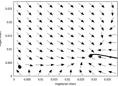
Figure 2 shows the differential field. The arrows represent the direction of change at

arrow indicates that vegetarianism is increasing and veganism is falling. There are

two equilibrium points where =0

dt dm_t

and =0

dt dh_t

, represented by circles on the

figure. The lower of the two is at (mt,ht) =(0.002,0.003), which is an unstable

equilibrium so that as a temporary campaign increases the rate of vegetarianism, the

rates of vegetarianism and veganism move towards the higher equilibrium

permanently. The higher equilibrium point is at (mt,ht)=(0.029,0.008), which is a

stable equilibrium so that as a temporary campaign increases the rate of vegetarianism

away from this equilibrium, the rates of consumption of the two diets subsequently

restore to the equilibrium rates. An example path by which restoration occurs after a

campaign raises mt to 0.034 is shown by the thick black line in the lower right of the

figure, with most of the adjustment occurring by a direct decline in the rate of

vegetarian consumption and a slight rise and fall in vegan consumption. The upper

equilibrium point is an attractor for all higher rates of vegetarianism and veganism as

well, so that there is no large single campaign that will result in a permanent trend

towards increased vegetarian and vegan consumption. The upper equilibrium point is

also is close to the current UK rates which have been fluctuating around the same

Figure 2. Differential field showing directions of movement in the vegetarian and vegan shares at

different values of the shares

0 0.005 0.01 0.015 0.02 0.025

0 0.005 0.01 0.015 0.02 0.025 0.03 0.035

V

e

g

a

n

s

h

a

re

Vegetarian share

The second type of vegetarian campaign is one that permanently alters the model

parameters, and so changes the equilibrium consumption of vegetarian and vegan

diets. These campaigns achieve persistent gains for animal rights, in contrast to the

transient effect of temporary campaigns. We calculate the effect of two permanent

campaigns. The first campaign performs more advertising for vegetarian diets to

attract people from both omnivorous and vegan diets. As given in equation (1), the

vegetarian percentage follows the dynamic equation

t t t

t t

t t

t t

h m f f l m a a m h d d m l c c dt

dm

) (

) (

) (

)

( ₀ + ₁ − ₀+ ₁ + ₀+ ₁ + ₀ + ₁

and the campaign raisesa0 (increasing adoption of vegetarian diets from omnivorous

diets) and f0 (increasing adoption of vegetarian diets from vegan diets). We

represent the changes by adding a small scalar quantity q to a0 and f0 . The

campaign may also be considered to reduce c₀ (lowering exits from vegetarian to

omnivorous diets) and d0 (lowering exits from vegetarian to vegan diets), but we

focus on the campaign as only attracting people to the vegetarian diet rather than

additionally discouraging them from leaving it. In the next campaign we consider, the

effects acting through a0 and f0 are isolated further.

After including q and transforming the dynamic equation as in section 2 we have

t t t t t t h m f d c a m c a h q f q a m d c c a q a q a dt dm ) ( ) ( ) ( ) ( 1 1 1 1 2 1 1 0 0 0 1 0 1 0 0 + − + − + + − + + + − − + − − − + − − + + = or t t t t t t h m f d c a m c a h f a m q d c c a a q a dt dm ) ( ) ( ) ( ) ( 1 1 1 1 2 1 1 0 0 0 1 0 1 0 0 + − + − + + − + + − + − − − − + − + + =

or in reduced coefficients

2 5 4

3 2

1 ) ( )

( t t t t t

t _{q q m h mh m}

dt

dm _{α α α α α}

The vegan percentage follows equation (2), or t t t t t t t t t m h d d l h b b h m f f h l e e dt dh ) ( ) ( ) ( )

( 0+ 1 − 0+ 1 + 0 + 1 + 0 + 1

−

= .

which, after including q, transforms into

2 1 1 1 1 1 1 0 1 0 1 0 0 0 0 ) ( ) ( ) ( ) ( t t t t t t h e b h m f e d b h q f e e b b m d b b dt dh + − + − + + − + − − − − + − + + − + =

or in reduced coefficients

2 5 4

3 2

1 t ( ) t t t t

t h h m h q m dt

dh _{=β +β + β − +β +β}

.

We solve the original equations (3) and (4) at their equilibrium points

0 2 5 4 3 2

1+ + + + =

= t t t t t

t _{m h mh m}

dt

dm _{α α α α α}

and 0 2 5 4 3 2

1+ + + + =

= t t t t t

t h h m h m dt

dh _{β β β β β}

which yields solutions in (m,h). We are interested in the solution (mS,hS) close to

their current rates, as the resulting analysis has most current policy relevance and it is

more likely to be relevant at rates close to those used in estimation. We solve again

for the perturbed equations under a value of q of 0.00001 to give corresponding

solutions (mS₊,hS₊). The differential of the change in mS and hS with respect to q

are approximated by dm_S/dq=(m_S+ −m_S)/q and dh_S/dq=(h_S+−h_S)/q , which

describe the relative responses of the percentage of vegetarians and vegans to the

campaign. These allow us to say how many people adopt a vegan diet following a

campaign which persuades one extra person to adopt a vegetarian diet at equilibrium,

using the quantity (dh_S/dq)/(dm_S/dq).

The second campaign also performs more advertising for vegetarian diets but attracts

people from omnivorous diets alone, leaving the direct movement from vegan diets

unchanged. In the dynamic equation (1) for vegetarian numbers

t t t t t t t t t h m f f l m a a m h d d m l c c dt dm ) ( ) ( ) ( )

( 0 + 1 − 0+ 1 + 0+ 1 + 0 + 1

− =

the campaign is represented by an increase in a0 alone. Including q and transforming

the dynamic equation as in section 2 gives

t t t t t t h m f d c a m c a h f q a m d c c a q a q a dt dm ) ( ) ( ) ( ) ( ) ( 1 1 1 1 2 1 1 0 0 0 1 0 1 0 0 + − + − + + − + + − − + − − − + − − + + =

2 5 4

3 2

1 ) ( ) ( )

( t t t t t

t _{q q m q h mh m}

dt dm α α α α

α + + − + − + +

= .

The vegan share follows equation (2)

t t t t t t t t t m h d d l h b b h m f f h l e e dt dh ) ( ) ( ) ( )

( 0+ 1 − 0+ 1 + 0 + 1 + 0 + 1

− =

which is unchanged under the campaign. In reduced coefficients, the equation

remains 2 5 4 3 2

1 t t t t t

t h h m h m dt dh β β β β

β + + + +

= .

We then proceed in the same way as for the first campaign to calculate differentials of

numbers of vegetarians and vegans, and the change in the number of vegans when the

campaign increases the number of vegetarians by one. All campaign effects are

calculated at the equilibrium close to the current rates of vegetarian and vegan

consumption.

Only the central estimates of campaign response are reported. We could sample from

the distribution of the parameter estimates to get alternative parameters for differential

equations (3) and (4) and their linearised forms, which would be solved to find any

equilibrium points. The equilibrium points at the campaign perturbed parameters

be repeated to obtain a distribution for the policy responses. However, the size of the

uncertainty in the parameter estimates produces some serious problems with the

practical implementation of the procedure. The simultaneous quadratic equations

which are solved to give the equilibrium points may have multiple solutions and there

may be ambiguity about which one should be considered for calculating the campaign

response, particularly if the solutions lie far from the current level of vegetarian and

vegan consumption. Some parameterisations may not have any equilibrium points,

with no campaign response available for calculation. We therefore only observe that

there is wide uncertainty in the campaign response.

Table 2. Equilibrium shares and responses to vegetarian campaigns

Model Full Linear Full Linear

Estimation method SUR SUR EKF-CT/DO EKF-CT/DO Equilibrium share

Vegetarians 0.029 0.030 0.029 0.029 Vegans 0.008 0.010 0.009 0.009 Campaign one to boost the vegetarian diet at the expense of the omnivorous and vegan diet Change in number of vegans

per extra vegetarian 0.35 0.37 0.32 0.29 Campaign two to boost the vegetarian diet at the expense of the omnivorous diet Change in number of vegans

per extra vegetarian 0.36 0.38 0.33 0.30

Campaign three to boost the vegan diet at the expense of the omnivorous and vegetarian diet Change in number of

vegetarians per extra vegan 0.76 0.77 0.50 0.53

Table 2 shows the results. The full and linear specifications, estimated under the SUR

and EKF-CT/DO, have close agreement on the equilibrium level of consumption with

current parameters. They put the equilibrium vegetarian consumption at around 2.9

percent of the total population, and equilibrium vegan consumption at around 0.9

percent of the population. There is slightly wider divergence in the effect of the

campaigns, but they are still similar. In the case of the campaign one to increase

vegetarian is associated with between 0.29 and 0.37 extra vegans, depending on the

model and estimation method. The campaign is associated with growth in

consumption of the vegan diet despite it directly attracting people to vegetarianism

from veganism. The reason is that the campaign also attracts people from the

omnivorous diet to a vegetarian diet, and some of them then move to a vegan diet. As

the equilibrium number of omnivores is much larger than the number of

non-omnivores, many more people move from the omnivorous diet to a vegetarian one and

then a vegan one than leave a vegan diet to adopt a vegetarian one. Thus, the net

effect of the campaign is to increase the number of vegans.

In the case of the campaign two to increase vegetarian consumption by attracting from

an omnivorous diet alone (and not a vegan one), each extra vegetarian is associated

with an additional 0.30 to 0.38 vegans depending on the model and estimation method.

This campaign has very little additional effect on vegan numbers compared with the

campaign that also attracts from veganism. The reason is that the effect of the

campaign is largely determined by the movement from the omnivorous diet to a

vegetarian and then vegan diet. The numbers of people that the campaign encourages

to abandon veganism for vegetarianism is small, so their exclusion does not alter net

campaign effects.

Some campaigners have called for the resources spent on animal welfare campaigns

to be redirected towards vegan campaigns, such as Gary-TV (2015). Our model

allows us to see how the numbers of vegetarians would change in response to a

omnivores and vegetarians to veganism, and is represented algebraically in the

dynamic equations (1) and (2)

t t t t t t t t t h m f f l m a a m h d d m l c c dt dm ) ( ) ( ) ( )

( 0 + 1 − 0+ 1 + 0+ 1 + 0 + 1

− = and t t t t t t t t t m h d d l h b b h m f f h l e e dt dh ) ( ) ( ) ( )

( 0+ 1 − 0+ 1 + 0 + 1 + 0 + 1

− =

by increases of q in b0, the rate of externally induced adoption of the vegan diet from

the omnivorous diet, and in d0, the rate of externally induced adoption of the vegan

diet from the vegetarian diet. After transformation and including the campaign

parameter q, equation (3) describing the number of vegetarians becomes

t t t t t t h m f d c a m c a h f a m q d c c a a a dt dm ) ( ) ( ) ( ) ( 1 1 1 1 2 1 1 0 0 0 1 0 1 0 0 + − + − + + − + + − + − − − − + − + =

and equation (4) describing the number of vegans becomes

2 1 1 1 1 1 1 0 1 0 1 0 0 0 0 ) ( ) ( ) ( ) ( t t t t t t h e b h m f e d b h f e e b q b m d b q b dt dh + − + − + + − + − − − + − − + + − + + =

2 5 4

3 2

1 ( ) t t t t t

t _{q m h mh m}

dt

dm _{α α α α α}

+ +

+ − +

= .

and

2 5 4

3 2

1 ) ( )

( t t t t t

t

h h m h

q m

q dt

dh _{= β + +β + β − +β +β}

.

The effect of the campaign is then calculated as for the other two campaigns, with

) / /( ) /

(dmS dq dhS dq estimating the change in the number of vegetarians when the

number of vegans increases by one.

The results are shown in table 2. Estimates of the change in vegetarian numbers vary

from 0.50 to 0.77, with the SUR estimates higher than the extended Kalman filter

estimates. The vegan campaign is nearly as effective at generating new vegetarians as

new vegans. Although the campaign results in people abandoning their vegetarian

diet in favour of a vegan one, the movement from the omnivorous diet to the vegan

diet is much larger in scale. Some of these new vegans subsequently adopt a

vegetarian diet, and this movement is larger than the one in the other direction.

6. Conclusion

Our work indicates that vegetarian campaigns increase vegan numbers, and a

policy-relevant question that follows this conclusion is whether an animal use abolitionist

who only cared about vegan numbers could support a vegetarian campaign. To

a vegetarian diet through a vegetarian campaign, then the cost of one person adopting

a vegan diet through the same campaign is about C₁/0.34≈2.94C₁. If it costs C₂ to

persuade someone to adopt a vegan diet through a vegan campaign, then the

abolitionist should prefer the vegetarian campaign route if and only if 2.94C₁ <C₂.

Similar calculations can be made under other valuations, such as one that attributed a

non-zero value to a vegetarian adoption.

This inequality ignores certain concerns of abolitionists. Among them is the

entrenchment of use of animal products by non-vegan campaigns, which in our model

would be represented by a decline in the transition rates into veganism in response to

such campaigns. We didn’t look fully at this dynamic link, so we can’t exclude the

possibility. Future work could examine whether it occurs and how critical it is,

perhaps using the parameter tracking of the extended Kalman filter as in Naik et al

(2008).

Our work points to a problem for the animal rights movement in the UK. Vegetarian

and vegan numbers are now close to their equilibrium rates, and those equilibria have

not changed much over the last twenty years. The recent flattening in the growth rates

of the numbers of vegetarians and vegans is not the result of a failure or change of

strategy, but an attainment of the potential of the advocacy approach followed over

the same period. To move to a much higher rate requires a substantial adjustment to

the approach.

This is not to say that it is a good idea to abandon the advertising, lobbying, and

advocacy since the 1990s. Their loss would result in declines in the level of veganism,

and constraints on them such as “ag-gag” laws (prohibiting disclosure of information

about malpractices inside agricultural establishments by whistleblowers) should be

challenged. The problem is in large part the overwhelming advertising and consumer

access advantages of animal product industries. Even the largest animal rights

organisations have tiny budgets by comparison (Counting Animals, 2015), and the net

transition from omnivorous to non-omnivorous diets is commensurately small

(Chintagunta and Vilcassim (1992) argue the transition coefficient in a duopoly is

proportional to the square root of advertising expenditure). It may be helpful to

analyse funding models in which a dominant good is supported by self-sustaining

sales revenue and a substitute good is supported by charitable donations, to see if

asymmetric positions can be used to the advantage of vegan promotion, rather than

primarily hindering it.

Recent innovative campaigns have tried to adjust the word-of-mouth influence of

people following vegetarian and vegan diets, rather than just the external advertising

examined here. For example, a recent campaign Gary-TV (2015) relied on

word-of-mouth diffusion over internet social media with periodic central intervention by the

campaign coordinators. Another campaign, Direct Action Everywhere (2015),

encourages its supporters to undertake high visibility actions and tell other people

about cruelties in animal production without primarily focussing on the direct

promotion of veganism. We could represent this in our model by increased

word-of-mouth influence by vegetarians and vegans, but also by sympathetic omnivores who

model may have stochastic connections between people and greater weak link

formation due to the campaign (see Goldenberg et al, 2001).

There are some refinements in the empirical approach used in this paper that would be

very welcome. The SUR method neglects the continuous nature of the underlying

model, while the extended Kalman filter method has high levels of parameter

uncertainty. A method that simultaneously solved these two problems would allow

sharper results and interpretations. It is possible that the problem is primarily of

colinearity in the specification, and that the full model given here should be reduced

to the smaller Case (1979) model which does have high parameter significance, or

another smaller alternative model used.

The theoretical model could be revised in various ways to make fuller use of the data

or reflect contemporary developments in animal rights advocacy. Classifying people

as omnivores, vegetarians, or vegans neglects the extent of use of animal products.

Some animal advocates call for meat reduction to be a campaign target (Fischer and

McWilliams, 2015; Ball, 2015). Meat and dairy use, and the effect of campaigns on

them, could be examined in a bivariate or trivariate model. The wider arguments in

the animal rights community on campaigns for animal welfare reforms and the

Appendix A

The Extended Kalman Filter in continuous time with discrete observations (EKF-CT/DO)

The continuous time and discrete observation extended Kalman filter has been

previously used by Xie et al (1997), who use filter projection for simultaneous

Bayesian updating of parameter estimates and sales, and Naik et al (2008) who use it

to determine the behaviour of endogenous consumer awareness in a dynamic

oligopoly. In contrast, our approach takes the parameters outside of the state variable,

making them amenable to classical estimation and limiting the impact of prior beliefs

on their assessment.

The extended Kalman filter with continuous time and discrete observations applies to

state space models of the form

t t t t dt d

v u

ξ

f

ξ

+ = ( , )

t t t h ξ w z = ( )+

where ξt is a state vector of variables at time t some of which may be unobserved,

t

u is a vector of exogenous variables,

t

z is a vector of observed variables,

f and h are differentiable functions,

and vt and wt are mutually uncorrelated white noise with contemporaneous error

variances of t

T t t

E(v v )=Q and t

T t t

After initialisation the filter has two repeated stages, consisting of successive

forecasting and updating. In the first stage at time t using the information available at

that time, the state variable is forecasted to give a value of ξt+1|t and the mean squared

error is forecasted to 1| (( 1 1|)( 1 1| ) )

T t t t t t t t

t+ =E ξ+ −ξ+ ξ + −ξ+

P . At the second stage, the

forecasts are updated using information available at time t+1 to give ξt+1|t+1 and

1 | 1 + + t t

P . We describe each stage more fully next.

Estimates are made of the starting state vector ξ0|0 and its mean squared error P0|0

with information available at time 0. For forecasting at time t and starting from

t t t ξ|

ξ = and Pt =Pt|t, we iteratively calculate at small intervals from time t to t+1 the

equations

dt dξt =f(ξt,ut)

dt dP_t =(F_tP_tT +P_tF_tT +Q_t)

where Ft =df/dξtT is the Jacobian of f evaluated at (ξt,ut) . In our data, we

calculate at ten steps between each data point. The final values give the forecasted

state vector of ξt+1|t and mean squared error of Pt+1|t. They are then used to derive the

forecasted observed vector zt+1|t and its mean squared error MSE(zt+1|t) from the

equations

t t t t

t+1| =H+1ξ+1|

z

1 1

| 1 1 |

1 )

( ₊ = _{+ + +} + t₊

T t t t t t t

where T t dh dξ

H+1 = / is the Jacobian of h evaluated at ξt+1|t.

For updating the state forecasts at time t+1 we use the Kalman formulae

)) (

( 1 1|

1 |

1 1 |

1t t t t t t t

t+ + =ξ+ +K+ z+ −h ξ + ξ t t t t t

t+1|+1 =(I−K +1H+1)P+1|

P

where I is the identity matrix with column and row dimension equal to the number of

variables in the state vector ξt, and

1 1 1 | 1 1 1 | 1

1 ( )

− + + + + + +

+ = + t

T t t t t T t t t

t P H H P H R

K

Our model can be represented in a state space form suitable for use in the filter:

t t v v =

t t ξ z =

t t ξ ξ h( )=

     

= 0 0

t w

The Jacobian of f is calculated numerically.

In our empirical model, errors occur only in the state equation rather than the

observation equation. Errors accumulate over time, as in empirical specifications of

diffusion due to Bass (1969), Schmittlein and Mahajan (1982), Srinivasan and Mason

(1986), Jain and Rao (1990), and Basu et al (1995). Our model is heavily

parameterised, and the restriction on the observation errors reduces the number of

parameters and improves convergence.

The updating phase of the Kalman filter allows us to track the likelihood function

generated by our model and data, which we use in maximum likelihood estimation of

Appendix B

SUR parameter estimates for the linearised model, over five year rolling periods of estimation

Dependent variable Change in vegetarian percentage Change in vegan percentage

Variable Vegetariant-1 Vegant-1 Constant Vegetariant-1 Vegant-1 Constant

Data 1992-1996 -0.877 0.577 0.020 0.175 -0.610 0.000

period 1993-1997 -1.146 0.152 0.029 0.088 -0.839 0.002

1994-1998 -0.927 0.393 0.022 -0.050 -0.956 0.007

1995-1999 -0.826 0.129 0.021 -0.105 -0.896 0.009

1996-2000 -0.930 0.504 0.022 -0.097 -0.793 0.008

1997-2001 -1.012 0.428 0.025 0.036 -0.945 0.006

1998-2002 -1.008 0.278 0.026 0.063 -1.293 0.009

1999-2003 -1.153 0.005 0.033 0.031 -1.321 0.010

2000-2004 -1.190 0.182 0.035 0.137 -1.092 0.005

2001-2005 -1.109 -0.426 0.038 0.124 -1.037 0.006

2002-2006 -1.019 0.171 0.029 0.116 -1.032 0.007

2003-2007 -1.068 -0.077 0.034 0.156 -1.038 0.007

2004-2008 -1.070 0.032 0.034 0.195 -1.056 0.006

2005-2009 -1.142 0.582 0.028 0.279 -1.087 0.004

2006-2010 -1.352 0.673 0.035 0.224 -0.914 0.003

2007-2011 -1.267 0.380 0.037 0.291 -0.600 -0.003

Appendix C

Data, prior to conversion to percentages

year qtr omnivores vegetarians vegans

1992 1 1843 38 9

1992 2 1820 39 12

1992 3 1778 39 13

1992 4 1783 36 7

1993 1 1768 41 8

1993 2 1675 51 3

1993 3 1616 38 6

1993 4 1719 41 10

1994 1 1696 43 4

1994 2 1756 41 7

1994 3 1608 52 8

1994 4 1658 39 15

1995 1 1616 44 9

1995 2 1673 46 6

1995 3 1649 43 14

1995 4 1623 44 11

1996 1 1650 29 9

1996 2 1571 35 9

1996 3 1568 50 9

1996 4 1490 42 8

1997 1 1579 49 5

1997 2 1611 44 7

1997 3 1527 46 12

1997 4 1504 49 9

1998 1 1565 28 7

1998 2 1608 36 12

1998 3 1598 39 17

1998 4 1583 52 8

1999 1 1618 48 11

1999 2 1679 50 19

1999 3 1784 47 17

1999 4 1750 40 9

2000 1 1641 43 18

2000 2 1576 59 14

2000 3 1681 43 12

2000 4 1537 44 12

2001 1 1600 51 8

2001 2 1719 72 16

2001 3 1816 46 22

2001 4 1836 66 13

Data, prior to conversion to percentages (continued) year qtr omnivores vegetarians vegans

2002 2 1643 33 10

2002 3 1697 57 17

2002 4 1652 54 11

2003 1 1688 47 18

2003 2 1732 44 15

2003 3 1644 63 20

2003 4 1678 56 13

2004 1 1713 54 16

2004 2 1518 65 14

2004 3 1685 65 19

2004 4 1622 65 17

2005 1 1672 32 24

2005 2 1580 51 14

2005 3 1564 48 22

2005 4 1726 44 22

2006 1 1655 49 10

2006 2 1618 50 24

2006 3 1580 61 19

2006 4 1515 42 22

2007 1 1407 50 17

2007 2 1409 42 16

2007 3 1535 53 20

2007 4 1504 62 21

2008 1 1384 41 21

2008 2 1361 50 16

2008 3 1443 54 18

2008 4 1397 42 16

2009 1 1409 44 13

2009 2 1394 38 16

2009 3 1415 53 15

2009 4 1376 35 14

2010 1 1233 38 9

2010 2 1288 43 11

2010 3 1299 48 16

2010 4 1217 47 14

2011 1 1309 39 17

2011 2 1343 50 11

2011 3 1402 45 16

2011 4 1401 48 10

2012 1 1361 48 10

2012 2 1371 41 20

2012 3 1301 44 19

References

Animal Aid, 2015. March is Veggie Month. Accessed at

http://www.veggiemonth.com/ on 13th September 2015.

Ball, M., 2015. Understanding the Numbers for Better Advocacy. Accessed at

http://www.mattball.org/2015/08/understanding-numbers-for-better.html on 13th

September 2015.

Bass, F.M., 1969. A New Product Growth Model for Consumer Durables. Marketing

Science 15, 215-227.

Beardsworth, A., Bryman, A., 2004. Meat consumption and meat avoidance among

young people: An 11 year longitudinal study. British Food Journal 106, 313-327.

Bennett, R., 1995. The value of farm animal welfare. Journal of Agricultural

Economics 46, 46-60.

Case, J.H., 1979. Economics and the Competitive Process. New York University

Press.

Chintagunta,, P.K., Vilcassim, N.J., 1992. An Empirical Investigation of Advertising

Strategies in a Dynamic Duopoly. Management Science 38, 1230-1244.

Chintagunta, P.K., Jain, D.C., 1995. Empirical Analysis of a Dynamic Duopoly

Model of Competition. Journal of Economics & Management Strategy 4, 109-131.

Counting Animals, 2015. Meat industry advertising. Accessed at

http://countinganimals.com/meat-industry-advertising/ on 13th September 2015.

DeCoux, E.L., 2009. Speaking for the modern Prometheus: the significance of animal

suffering to the abolition movement. Animal Law 16, 9-64.

Direct Action Everywhere, 2015. The Open Model. Accessed at

http://directactioneverywhere.com/theliberationist/2013/11/15/openness on 13th

Dunayer, J., 2004. Speciesism. Ryce Publishing.

Fastenberg, D., 2010. Weekday Vegetarians. Time Magazine online. Accessed at

http://content.time.com/time/magazine/article/0,9171,2010180,00.html on 13th

September 2015.

Fischer, B., McWilliams, J., 2015. When Vegans Won’t Compromise. New York

Times Online. Accessed at

http://opinionator.blogs.nytimes.com/2015/08/16/when-vegans-wont-compromise on 13th September 2015.

Francione, G.L., 1997. Animal rights theory and utilitarianism: relative normative

guidance. Animal Law 3, 75-101.

Francione, G., 2015. Veganism, PETA, Farm Sanctuary, Peter Singer, “Personal

Purity,” and Principles of Justice. Accessed at

http://www.abolitionistapproach.com/veganism-peta-farm-sanctuary-peter-singer-personal-purity-principles-justice on 13th September 2015.

Frank, J., 2006. Process attributes of goods, ethical considerations and implications

for animal products. Ecological Economics 58, 538-547.

Garner, R., 2006. Animal welfare: a political defense. Journal of Animal Law and

Ethics 1, 161-174.

Gary-TV, 2015. Gary-TV. Accessed at http://www.gary-tv.com/en/ on 13th September

2015.

Givon, M., Mahajan, V., Muller, E., 1995. Software Piracy: Estimation of Lost Sales

and the Impact on Software Diffusion. Journal of Marketing 59, 29-37.

Goldenberg, J., Libai, B., Muller, E., 2001. Talk of the Network: A Complex Systems

Look at the Underlying Process of Word-of-Mouth. Marketing Letters 12, 211-223.

Libai, B., Muller, E., Peres, R., 2009. The Diffusion of Services. Journal of Marketing

Naik, P.A., Prasad, A., Sethi, S.P., 2008. Building Brand Awareness in Dynamic

Oligopoly Markets. Management Science 54, 129-138.

Peta, 2015. Ideas for Vegetarian Living. Accessed at

http://www.peta.org/living/food/making-transition-vegetarian/ideas-vegetarian-living/ on 13th September 2015.

Schmittlein, D.C., Mahajan, V., 1982. Maximum Likelihood Estimation for an

Innovation Diffusion Model of New Product Acceptance. Marketing Science 1,

57-78.

Sorger, G., 1989. Competitive Dynamic Advertising: A Modification of the Case

Game. Journal of Economic Dynamics and Control 13, 55-80.

Srinivasan, V., Mason, C.H., 1986. Nonlinear Least Squares Estimation of New

Diffusion Models. Marketing Science 5, 169-178.

Vegetarian Society, 2015. National Vegetarian Week 2015. Accessed at

http://www.nationalvegetarianweek.org/ on 13th September 2015.

Waters, J., 2015. Ethics and the choice of animal advocacy campaigns. Ecological

Economics 119, 107-117.

Wrenn, C., 2012. Abolitionist animal rights: critical comparisons and challenges

within the animal rights movement. Interface 4, 438-458.

Xie, J., Song, X, Sirbu, M., Wang, Q., 1997. Kalman Filter Estimation of New

R language code implementing the estimation method

The code can be pasted directly into an R program, and requires the packages MASS,

numDeriv, and systemfit. It runs using the data in appendix C which should be saved

as UK_diet_rates.csv (for example as a csv file from a spreadsheet), for opening by

the R code. Line 11 in the code is

data<-read.csv("C:\\Documents\\UK_diet_rates.csv", header=T)

and the directory will have to be changed to where UK_diet_rates.csv has been saved.

Line four in the code is

.libPaths("C:/Documents/R/win-library/3.1")

and the directory will have to be changed to the local library directory for R. Type

.libPaths()

to see the current library directory.

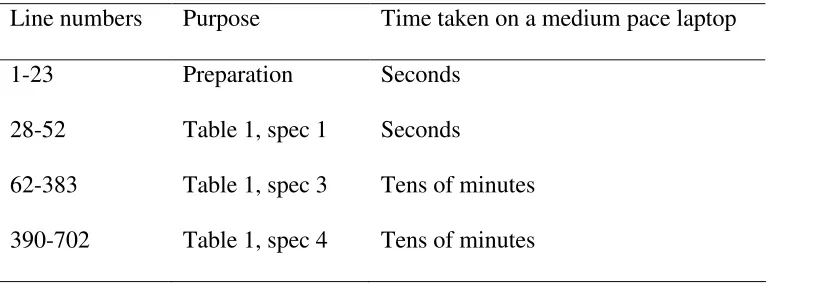
The code structure is shown in the table. The preparation section should been run first,

then any of the other sections can be run separately.

Line numbers Purpose Time taken on a medium pace laptop

1-23 Preparation Seconds

28-52 Table 1, spec 1 Seconds

62-383 Table 1, spec 3 Tens of minutes

390-702 Table 1, spec 4 Tens of minutes

The code for the extended Kalman filter has *not* been extensively tested as at 17th

September 2015. I’m uneasy about the convergence of the full model (table 1,