Trust and Economic Performance: A Panel Study

Munich Personal RePEc Archive

Trust and Economic Performance: A

Panel Study

Xin, Guangyi

University of Leicester

6 September 2017

Online at

https://mpra.ub.uni-muenchen.de/80815/

1

Trust and Economic Performance:

A Panel Study

Guangyi Xin

1

University of Leicester

Abstract

This paper critically reviews the current various measures of trust through surveys/questionnaires and trust experiments. The main shortcoming from such approaches is that the trust index produced from surveys and experiment are ambiguous. Given these arguments, I use Factor Analysis technique to construct a new trust index that account for indicators of degree of trust. Consequently, the rankings of countries in my index is more consistent compared to the rankings of existing trust indices. Using the above, I illustrate the panel analysis on the influence of trust on FDI inflows and income inequality. Trust turns out to play a significant role on FDI inflows. With regard to income inequality, trust is more pronounced among the OECD countries.

Keywords: Trust; Economic Performance; FDI inflow; Income Inequality

JEL Classification: C23; D63; O11; Z13

1

2

1 Introduction

In general, trust can be defined as a person’s belief in the integrity, reliability, and ability of others."Others" refers to either different (groups of) people or, more broadly, the various institutional aspects of the society in which a person lives (e.g., leaders and the quality of governance; law and order, etc.).

With respect to economics, trust can be seen as facilitating various aspects of economic activity. In particular, researchers have argued that trust can reduce transaction costs, promote cooperation, and encourage business activities (Knack and Keefer 1997). Therefore, economists claim that a higher level of social trust is positively correlated with economic development (Moegan and Hunt 1994). Put differently, it has been widely accepted and demonstrated that social trust benefits the economy and that a low level of trust inhibits economic growth.

3 advantageous outcomes (Uslaner 2003).

The earliest related literature analyses social capital, including trust, and the impacts of social capital on government performance across regions in Italy (Banfield 1958; Coleman 1988; Gambetta 1988; Putnam et al. 1993). Since those studies, the importance of trust to economic performance has drawn substantial attention. Therefore, the impact of trust on economic outcomes has been empirically investigated across different countries by Knack and Keefer (1997) and La Porta et al. (1997). The evidence also suggests that trust can promote financial development, effectively facilitate economic outcomes such as entrepreneurship and influence economic exchanges between two countries (Guiso et al. 2004, 2006, and 2009). Moreover, Bloom et al. (2007), Algan and Cahuc (2009) and Aghion et al. (2010) examine the correlation between trust and institutions.

Furthermore, the theoretical foundations of the effect of trust on the economy have been provided by Zak and Knack (2001). They present a model in which the rate of investment is determined by the level of trust. In their model, trust is characterised as the time that agents allocate to production rather than verifying others’ trustworthiness. Thus, this model effectively illustrates how different levels of trust determine economic performance. It also demonstrates the existence of a low-trust poverty trap. According to the model, trust depends on the institutional, economic and social environment. Specifically, trust is positively correlated with the institutional environment and economic conditions but negatively correlated with population heterogeneity.

4

of trust are conducted by assessing the average responses as “try to be fair” and “can be trusted” to the corresponding survey questions. The survey results are either used as the alternative measurement of trust or as the indicators of moral values (Tabellini 2010; Guiso et al., 2011).

However, the surveys can be interpreted differently due to the polysemy of the questions and responses (Algan and Cahuc 2013). Moreover, the respondents who claim to have high trust in others may behave differently in the reality (Algan and Cahuc 2013). In addition, there is always the risk that survey data contain systematic measurement errors, which can be either self-reported errors that are constant for each respondent over time or answers from a small group of people with particular personality traits that may not be informative about their corresponding behaviour (Zak 2005). Finally, the lack of WVS data on trust for less developed countries hinders the investigation into trust in these countries and often makes inter-temporal comparisons and cross-country studies infeasible.

To improve the measurement of trust, some researchers have conducted laboratory experiments that usually apply the “trust game” raised by Berg et al. (1995) or its variants.

Earlier studies demonstrate that the correlation between the answers to the trust survey and the behaviours in the experiment are mixed. For example, Glaeser et al. (2000) reveal that the answers to the trust survey are inconsistent with the behaviour in experiments. However, Holm and Danielson (2005) suggest that the answers to the trust survey and the behaviour in experiments are positively correlated in some countries, such as Sweden. Fehr et al. (2002) compare the results from the representative survey and representative behavioural data from a social dilemma experiment in Germany to illustrate that the trust question can measure the behaviour of trust but not trustworthiness. Meanwhile, Ermisch et al. (2009) show that the trust survey cannot predict behaviour in the trust experiment by conducting a real monetary rewards experiment on a sample of the British population.

5

indicate the degree of trust, particularly in reference to a financial or commercial relationship. Since the self-reported trust levels from the surveys and the actual behaviour in trust experiments are ambiguous, this paper follows the second approach to construct a new trust index by considering social and institutional characteristics as well as the educational and socioeconomic conditions that have been shown to affect trust levels.

This analysis is a systematic attempt to construct an alternative measure of trust. It also contributes to the literature by using a panel study to illustrate the effect of trust on economic performance variables. The three main objectives are to construct a new trust index by applying a factor analysis (FA) technique, to compare the new trust index to the previous measures of trust (trust survey), and to investigate the correlation between trust and foreign direct investment (FDI) inflows as well as income inequality.

The remainder of this paper is organised as follows. Section 2 illustrates the components of the trust index, the FA technique, and how FA can be used to construct the trust index. Section 3 compares the trust index to the trust survey measurement. Section 4 describes the application of the trust index by examining the correlation between the trust index and economic performance variables, such as FDI inflows and income inequality. Section 5 concludes this paper by discussing its main findings and limitations.

2 Trust index

This section explains the process of generating the trust index. The first subsection illustrates the components used to build the trust index. The theoretical foundations and empirical evidence for each component are discussed. In the second subsection, an FA technique is introduced and applied to assign weightings to all the components. Lastly, the third subsection presents the trust index built by the FA technique for 136 countries and reveals its validity.

2.1 Components of the trust index

6

and social relationships on trust (Arrow 1972; Putnam et al. 1993; Knack 2002; Uslaner 2002). Additionally, Glaeser et al. (2002) propose an economic approach to trust and demonstrate the correlation between trust and economic growth. I consider both economic and non-economic indicators in terms of degree of trust to generate a proxy. Therefore, my trust index would include three aspects: institutional environment; population heterogeneity; and educational and socioeconomic conditions, which are also consistent with the theoretical work of Zak and Knack (2001).

Most of the components I use to generate the trust index are drawn from the International Country Risk Guide (ICRG) dataset. The ICRG generates data concerning the ratings of political, economic and financial risks by using approximately 30 metrics based on original indicators. As a result, the generated data have different score points describing the scenarios for each country in each year. Here, I mainly employ the political rating data.

2.1.1 Institutional environment

For the institutional environment, I employ the index of property rights introduced by Knack and Keefer (1995). The index of property rights is produced by equally weighing four indicators from the ICRG: quality of bureaucracy, law and order,

7

system. Specifically, corruption is assessed in terms of “excessive patronage, nepotism, job reservations, ‘favour-for-favours’, secret party funding, and suspiciously close ties between politics and business”. Higher ratings are given to countries in which special payments make no difference to the government officials, while the lower ratings are given to the countries with serious corruption problems. Investment profile examines the possible risks to investments that are not caused by other political, economic or financial risk components. This indicator mainly consists of “contract viability/expropriation”, “profits repatriation” and “payment delays”. Investment profile is scored from 0 to 12 with higher scores implying a lower risk to investment. The scores of the index of property rights range from 0 to 28. Higher scores indicate a country’s governmental institutions are more effective, guaranteeing property rights and contract enforcement.

Knack and Keefer (1997) suggest that trust can be created by formal institutions such as a strong rule of law. Essentially, citizens tend to rely on informal and local rules in a weak legal enforcement environment, which nourishes particularised trust within a close social circle while simultaneously weakening generalised trust. The Mafia in Sicily vividly demonstrates the evolution of particularised trust under weak legal enforcement. Gambetta (1993) states that legal enforcement was very weak in Sicily around 1812 since the abolition of feudalism took place much later there than in the rest of Europe. As the state was unable to protect private property rights there, the Mafia took advantage by providing informal local protection. This local protection through patronage clearly treats those under the protection differently from everyone else. Without legal institutions and civic-minded officials, generalised trust can be damaged (Rothstein 2011). In the same vein, Guiso et al. (2008) note that weak legal enforcement in the distant past in some regions of Italy is still associated with a lower level of trust today.

8

accountability and corruption, as well as the effectiveness of property rights protection, rule of law and contract enforcement.

Moreover, Tabellini (2008) uses a novel way to verify the casual effect of institutional quality on trust. Specifically, he documents the correlation between the trust level of US immigrants and the institutional environment of their country of origin.

Recently, Algan and Cahuc (2013) illustrate the strong correlation between trust and institutional system by empirically investigating a sample of 100 countries. They also find a similar positive correlation between trust and governance quality in 163 European regions.

2.1.2 Population heterogeneity

In terms of population heterogeneity, I use measures of ethnic tensions, religious tensions and internal conflict from the ICRG. The scores of both ethnic tensions and

religious tensions range from 0 to 6 with a low rating reflecting high tensions.

9

Ritzen and Woolcock (2000), Woolcock et al. (2006) and Baliamoune-Lutz (2009) emphasise that the essential element of trust is social cohesion. Social cohesion is defined by Ritzen and Woolcock (2000) as “a state of affairs in which a group of people have an aptitude for collaboration that produces a climate for change”. This definition suggests that ethnic tensions can be a proxy for social cohesion because social cohesion not only reflects the popular observance of policy reforms but also affects the institutional implementation of those reforms. Additionally, ethnic fractionalisation might lead to the social exclusion of specific ethnic groups or even evoke a civil war (Woolcock et al. 2006; Baliamoune-Lutz 2009). In the same vein, Putnam (2007) reveals that trust tends to decline where ethnic fractionalisation or segregation exist. He illustrates that trust is relatively low in ethnically diverse residential areas based on cross-cities studies. By investigating across US states, Alesina and La Ferrara (2000, 2002) provide similar evidence. The findings may be because people naturally prefer to trust others with similar backgrounds and are therefore inclined to place less trust in those who are different from them. Moreover, high ethnic tensions result in lower cooperation, as represented by collective actions such as funding and public goods (Alesina et al. 1999; Miguel and Gugerty 2005). This decline in cooperation might be primarily due to weakened collective action resulting from distinct preferences and the free rider problem within ethnically diverse areas.

The influence of religious tensions on trust is similar to the influence of ethnic tensions. Levi (1996) and Uslaner (2002) reveal that some groups may inhibit instead of improving generalised trust in people who are outside the group. Groups that reinforce the in-group identity, such as religious fundamentalists and racists, can undermine generalised trust. Stolle (2000) suggests that if the group members have strong within-group trust, then those group members tend to have less trust in outsiders over time.

10

associated with distrust. They claim that a history of conflicts impacts the trust (beliefs) of the agent. The agent then redefines their trust (beliefs) and passes it to the next generation. Therefore, conflicts such as civil wars and civil disorder could even result in the permanent collapse of trust. Additionally, the empirical research of Rohner et al. (2013) illustrates that the measure of average trust is negatively associated with the frequency of civil war after controlling for democracy and other covariates based on country-level statistics during the period 1981-2008. Similarly, by exploring the violence surrounding the 2007 Kenyan election in Africa, Dercon and Gutierrez-Romero (2010) indicate that violence undermines generalised trust. In the same pattern, Rohner et al. (2013) uncover the causal effects of internal conflicts on trust by using individual- and country-level data in Uganda during the period 2002-2004. These scholars provide the robust results of intense fighting, which damages generalised trust by using a variety of identification methods.

2.1.3 Education and socioeconomic conditions

I adopt socioeconomic conditions from the ICRG and secondary school enrolment from the World Bank as proxies. Socioeconomic conditions measures factors including “unemployment rate, consumer confidence and poverty”, which reflect the socioeconomic pressures at work and in society. The points range from 0 to 12. High ratings are given to countries in which the citizens live under good socioeconomic conditions. Secondary school enrolment (% of gross) measures the percent of students enrolled at the secondary school level regardless of age.

11 higher average education level.

Earlier studies have revealed that individuals in high socioeconomic conditions tend to have higher levels of generalised trust than those in low socioeconomic conditions (Brehm and Rahn 1997; Putnam 2000; Alesina and La Ferrara 2002; Subramanian et al. 2003; Kaasa and Parts 2008). Furthermore, Rothstein and Uslaner (2005) note that poverty, which is also captured by socioeconomic condition, could damage the social fabric since the poor would feel isolated and disrespected by others.

To construct an index of country-level trust, set of weights must be selected for each component. Rather than imposing arbitrary or equal weights, I apply an FA technique to let the data determine the weights directly. The statistical summary of each component can be seen in Appendix 1.

2.2 Factor analysis technique

2.2.1 Factor analysis

FA is a statistical methodology that aims to use a smaller number of latent variables to represent a larger number of observed variables (Lewis-Beck 1994). For example, after using FA, the variation within five observed variables can be represented by one or two unobserved variables (latent factors). FA can also be used to predict latent variables by investigating the joint variation within the observed variables. Using this technique, each observed variable can be modelled as a linear combination of the latent factors with the term “error”. Since the observed variables are interrelated, the set of variables can finally be reduced to a lower number of unobserved factors. FA was first used in psychometrics field, and it was later widely used in the social sciences, marketing and other applied economics research areas.

12

variance. Specifically, the components in PCA have orthogonal linear combinations, and they maximise the total variance. However, the factors in FA are linearly combined to maximise the shared fraction of the variance, namely, the latent construction. Thus, FA is suitable for testing a theoretical model of latent factors related to observed variables. With respect to simply reducing the number of current variables, PCA is more appropriate.

2.2.2 Statistical model

Suppose that in a dataset, we have a group of n observable random variables such as x", $%, … , $' with means (", (%, … ('. According to the above definition of

FA, after using this technique, we get some *_+, associated with k unobserved variables -,. The mathematical equation can be expressed as follows:

$₊− (₊ = *_+"-_"+ ⋯ + *₊₂-₂+ 3₊ (1) Here, 4 ∈ 1, … , 7, 8 ∈ 1, … , 9, and 9 < 7. The error term is 3₊ , which is independently distributed with a zero mean and finite variance. Here, Fs can be referred to as factors or latent unobserved variables. In addition, $< are observed variables. The equation simply conveys that we can use fewer factors to express the association among a higher number of observed variables by using FA techniques.

In particular, we have a common factor model or one factor model. In this case, it would be

$"− (" = *""- + 3"

$_% − (_% = *_%"- + 3_%

… (2)

$_' − (_' = *_'"- + 3_' where $< are the observed variables, F is the common factor, *s are associated

factor loadings and 3s are error terms or uniqueness.

2.2.3 Types

13

the hypothesis of the association between observed variables and unobserved variables. The most significant difference between these two techniques is whether a hypothesis concerning the association of the variables is introduced. Additionally, unlike exploratory FA, confirmatory FA is mainly used to predict latent factors and the associated structures in the original dataset.

2.2.4 Terminology

FA uses several specific terms. The first is factor loadings, which captures the correlation coefficients between the corresponding observed variables and latent factors. Additionally, the squared factor loading reveals the percentage of the variance that can be explained by the factor. The sum of the squared factor loadings for all factors for a given variable is called communality. Communality

measures the percentage of variance of a given variable that is explained jointly by all the latent factors, which can be an indicator of whether the model is suitable. The variance that cannot be accounted for by the latent factor is uniqueness, which equals one minus communality. Additionally, the number of factors are decided by the eigenvalue. Eigenvalue describes the variance explained by the latent factor, which indicates the explanatory power of the latent factor based on the variables. Thus, a higher eigenvalue indicates a more powerful latent factor. Specifically, the latent factor and its structure can express the set of observed variables more accurately. The last related term is factor scores. Factor scores refers to the scores of each set of variables on each factor. By using FA techniques, each observation eventually receives its respective scores. In addition, by multiplying the score by the associated observation, the latent variable value of this observation can be obtained.

2.2.5 Criteria for determining the number of factors

14

as Stata and SPSS. According to the Kaiser criterion, all the factors with eigenvalues below 1 will be dropped.

2.3 Construction of the Trust index using FA

I assume that one common factor can be used to explain the variance of trust. Each component is predicted to positively contribute to the “trust index”. Thus, I apply the confirmatory common factor model.

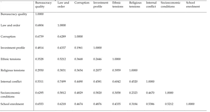
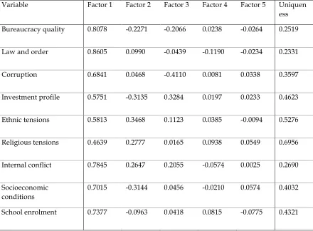
First, I illustrate the correlation matrix of the components, and the results are shown in Table 1. Second, the FA is applied and the eigenvalues for each possible factor and the corresponding factor loadings are collected. The FA output can be found in Table 2.a. According to the Kaiser criteria, the number of retained factors should be one, which is consistent with the assumption of the common factor model. To further verify the number of factors, the scree plot is illustrated and shown in Figure 1, which also suggests the common factor model.

Figure 1. Scree plot of eigenvalues after factor analysis

The factor loadings and the unique variances between each component and the factors are shown in Table 2.b. Since the retained number of factors is one, only

0

1

2

3

4

Ei

g

e

n

va

lu

e

s

0 2 4 6 8 10

Number

15

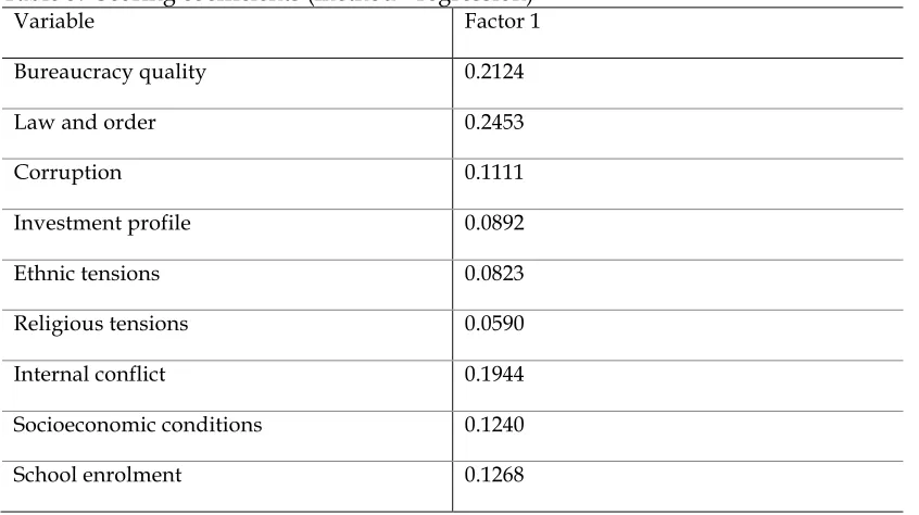
Factor 1 would be applied. The first column in Table 2.b illustrates how the common factor (Factor 1) captures each component. Specifically, the common factor “trust index” is positively correlated to each observed component. Moreover, the high factor loadings suggest the stronger contribution of latent factors to the observed components. I follow the majority of studies and use 0.3 as the limit (Comrey and Lee 1992; Hair et al. 1998). In my case, all the factor loadings are above 0.3, which means that the latent “trust index” effectively captures all the characteristics of the observed components. Finally, the factor scores for each component with a standardised unit are predicted using the regression scores method2_{. The scores are shown in Table 3, and all the}

components positively contribute to the trust index, which is consistent with the previous assumption. Among the components, law and order has the highest factor score, which indicates that a standardised unit increase in the law and order

component is associated with a 0.25 standardised unit increase in the latent “trust index”.

2 _{The maximum likelihood (ML) method is only one of several methods used for confirmatory factor analysis}

16

Table 1. Correlation matrix of the components

` Bureaucracy

quality

Law and order

Corruption Investment profile

Ethnic tensions

Religious tensions

Internal conflict

Socioeconomic conditions

School enrolment

Bureaucracy quality 1.0000

Law and order 0.6804 1.0000

Corruption 0.6739 0.6289 1.0000

Investment profile 0.4814 0.4337 0.1961 1.0000

Ethnic tensions 0.3528 0.5212 0.3668 0.2446 1.0000

Religious tensions 0.2930 0.3831 0.3654 0.2077 0.3959 1.0000

Internal conflict 0.5311 0.7499 0.4490 0.4581 0.6042 0.4520 1.0000

Socioeconomic conditions

0.6295 0.5812 0.4829 0.5820 0.3058 0.2323 0.4670 1.0000

17 Table 2. a. Factor analysis

Factor Eigenvalue Difference Proportion Cumulative

Factor 1 4.3966 3.8591 0.9112 0.9112

Factor 2 0.5375 0.1572 0.1114 1.0226

Factor 3 0.3803 0.3445 0.0788 1.1014

Factor 4 0.0358 0.0205 0.0074 1.1088

Factor 5 0.0153 0.0896 0.0032 1.1120

Factor 6 -0.0743 0.0274 -0.0154 1.0966

Factor 7 -0.1016 0.0686 -0.0211 1.0755

Factor 8 -0.1702 0.0240 -0.0353 1.0402

Factor 9 -0.1942 - -0.0402 1.0000

Table 2. b. Factor loadings (pattern matrix) and unique variances

Variable Factor 1 Factor 2 Factor 3 Factor 4 Factor 5 Uniquen ess

Bureaucracy quality 0.8078 -0.2271 -0.2066 0.0238 -0.0264 0.2519

Law and order 0.8605 0.0990 -0.0439 -0.1190 -0.0234 0.2331

Corruption 0.6841 0.0468 -0.4110 0.0081 0.0338 0.3597

Investment profile 0.5751 -0.3135 0.3284 0.0197 0.0233 0.4623

Ethnic tensions 0.5813 0.3468 0.1123 0.0385 -0.0094 0.5276

Religious tensions 0.4639 0.2777 0.0165 0.0938 0.0549 0.6956

Internal conflict 0.7845 0.2647 0.2055 -0.0574 0.0025 0.2690

Socioeconomic conditions

0.7015 -0.3144 0.0456 -0.0210 0.0574 0.4032

18 Table 3. Scoring coefficients (method= regression)

Variable Factor 1

Bureaucracy quality 0.2124

Law and order 0.2453

Corruption 0.1111

Investment profile 0.0892

Ethnic tensions 0.0823

Religious tensions 0.0590

Internal conflict 0.1944

Socioeconomic conditions 0.1240

School enrolment 0.1268

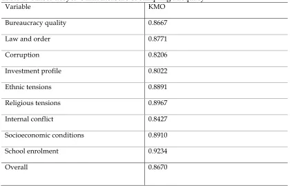
The acceptability of the common FA model has been confirmed based on three aspects. First, the overall goodness of fit is examined. The p-value of chi2 is close to zero, which indicates that the common FA model is meaningful. Second, the interpretability, strength, and statistical significance of the estimated parameters have been reviewed. In my case, the parameters are of a magnitude and direction consistent with expectations and the existing empirical evidence. Finally, the measures of sampling adequacy are checked by the Kaiser-Meyer-Olkin (KMO) test. Table 4 explains the KMO test results. Generally, the overall KMO test score must be above 0.5. The KMO value here is 0.867, which is considered a good indication of the usefulness and the adequate quality of the components and the FA model.

19

Table 4. Kaiser-Meyer-Olkin measure of sampling adequacy

Variable KMO

Bureaucracy quality 0.8667

Law and order 0.8771

Corruption 0.8206

Investment profile 0.8022

Ethnic tensions 0.8891

Religious tensions 0.8967

Internal conflict 0.8427

Socioeconomic conditions 0.8910

School enrolment 0.9234

Overall 0.8670

3 Comparison with trust survey results

20

the lowest with only 3.8% of the population trusting others. The full ranking list of trust levels measured by the WVS trust question can be seen in Appendix 2.

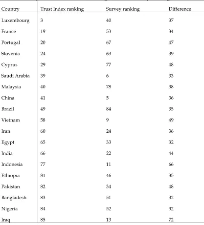
To compare the ranking of my trust index and the trust survey, I find 85 common countries from the above two samples and reorganise the rankings for these countries. Appendix 3 illustrates the comparisons of the rankings for these countries in terms of the two measures of trust identified above. I should emphasise that the rationale behind this comparison is informational purposes rather than making statements about how well my index corresponds to the “correct” ordering of a country’s trust level. I find some countries that illustrate very distinct rankings in the two indices (trust survey ranking and trust index ranking) and show them in Table 2.5. In the trust survey ranking, countries such as Luxembourg, France, Portugal, Slovenia, Cyprus and Malaysia surprisingly rank around and below the average level of trust, while relatively high trust levels have been found in China, Saudi Arabia, Vietnam, Indonesia, Iraq and India. In particular, Luxembourg ranks 40, placing it behind Vietnam (9) and India (22) in the trust survey ranking. However, in the trust index ranking, Luxembourg ranks 3, which is just behind Finland (1) and the Netherlands (2). Similarly, France ranks at 53, which is below the average trust level in the trust survey ranking; by contrast, it ranks 19 in the trust index, which places it in the top quarter. By contrast, China ranks 5 in the trust survey ranking, but it is just above the average trust level at 41 in the trust index ranking. Following the same pattern, Vietnam ranks 9 in the trust survey and 58 in the trust index ranking.

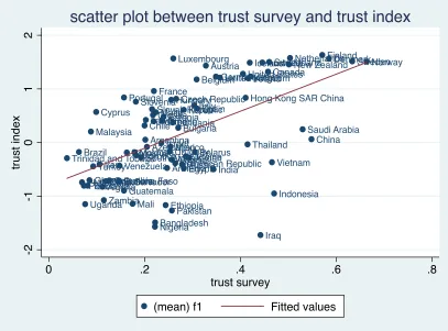
I further investigate the similarity between the trust index and the measurement of the trust survey. Initially, the scatter plot (Figure 2.2) between the measurement of the trust survey and trust index suggests an obvious positive correlation. This highly positive correlation has also been confirmed by Table 2.6. The value 3.456 reveals that the measurements of the trust survey are positively related to the trust index and are highly statistically significant. One additional standardised unit increase in the measure of the trust survey leads to an increase of 0.52 standardised units in the trust index.

21

level when the trust value is not available in the WVS.

Table 5. Subsample of the Trust Index ranking and Trust Survey ranking

Country Trust Index ranking Survey ranking Difference

Luxembourg 3 40 37

France 19 53 34

Portugal 20 67 47

Slovenia 24 63 39

Cyprus 29 77 48

Saudi Arabia 39 6 33

Malaysia 40 78 38

China 41 5 36

Brazil 49 84 35

Vietnam 58 9 49

Iran 60 24 36

Egypt 65 33 32

India 66 22 44

Indonesia 77 11 66

Ethiopia 81 46 35

Pakistan 82 34 48

Bangladesh 83 51 32

Nigeria 84 52 32

22

Figure 2. Scatter plot between measure of trust survey and trust index

Table 6. Pooled regression between trust survey and trust index Trust index

Trust survey 3.456***

(0.556)

Constant -0.799***

(0.171) Sample Size

R-square

85 0.3178 * p<0.10, ** p<0.05, *** p<0.01

Note: Trust index and trust survey are measured over the period 1984-2008.

4 The correlation between the trust index and economic

performance

Earlier studies mainly explore the cross-sectional effect of trust measured by the trust survey variable obtained from the WVS regarding economic activity variables such as GDP per capita and investment rate. Knack and Keefer (1997) suggest that the average trust level is strongly associated with GDP per capita across countries. Putnam et al. (1993) also document the cross-region effect of trust on economic development in Italy.

Albania Algeria Argentina Armenia Australia Austria Azerbaijan Bangladesh Belarus Belgium Brazil Bulgaria Burkina Faso Canada Chile China Colombia Croatia Cyprus Czech Republic Denmark Dominican Republic Egypt El Salvador Estonia Ethiopia Finland France Germany Ghana Greece Guatemala

Hong Kong SAR China Hungary Iceland India Indonesia Iran Iraq Ireland Israel Italy Japan Jordan Korea Latvia Lithuania Luxembourg Malaysia Mali Malta Mexico Moldova_Morocco Netherlands New Zealand Nigeria Norway Pakistan Peru Philippines Poland Portugal Romania Russia Saudi Arabia Slovak Republic Slovenia South Africa Spain Sweden Switzerland Tanzania Thailand Trinidad and Tobago

Turkey Uganda

Ukraine

United KingdomUnited States

Uruguay Venezuela Vietnam Zambia Zimbabwe -2 -1 0 1 2 tru st i n d e x

0 .2 .4 .6 .8

trust survey

(mean) f1 Fitted values

23

Cross-country studies on the effect of trust have also been conducted by La Porta et al.

(1997), Whiteley (2000), Zak and Knack (2001), Beugelsdijk et al. (2004), Bjørnskov (2006b), Knowles (2006), Berggren et al. (2008), Neira et al. (2009), Tabellini (2010), and Dincer and Uslaner (2010). There are fewer studies of panel data analysis on the correlation between trust and economic performance3_{, which could be due to the}

severe issue of missing observations of the trust data from the WVS and the estimation results based on that data tending to be not robust in the panel fixed effect model (Hall and Ahmad 2013). Therefore, I explore the effect of trust (measured by the trust index) on FDI and income inequality using a panel data analysis.

4.1 Trust and foreign direct investment (FDI)

Trust has been routinely considered to be an essential element for most economic transactions (Blau 1964). The impact of trust on economic growth has been widely investigated (such as Putnam et al. 1993; Knack and Keefer 1997; Woolcock 1998; Knowles 2006; Tabellini 2010; Algan and Cahuc 2013). While FDI is one of the most significant contributors to economic growth (Borensztein et al. 1998), the influence of trust on FDI has rarely been examined4_.

Trust could promote FDI mainly through two channels. First, a high level of trust effectively cultivates a cooperative business environment, which facilitates FDI activities. Trust has been seen as the “expectation of regular, honest cooperative behaviour” (Bhardwaj et al. 2007), which could lessen the probability of opportunism and strengthen the transparency of economic exchange (Bradach and Eccles 1989; Hill 1990). Earlier studies suggest that people are more likely to trust others in a society with a high trust level, which results in a cooperative relationship that facilitates economic achievement (Miller 1992; Mcknight et al. 1998; Das and Teng 2000). From the multinational enterprises’ perspective, a cooperative business environment in the host country is helpful to making FDI (Zhao and Kim 2011) profitable. Second, trust can enhance contract enforcement (Fukuyama 1995; Knack and Keefer 1997), which is mainly due to trust promoting compliance with property rights and business rules

3 _{There is limited research using panel data analysis on the effect of trust on economic growth; see, for example,} Perez et al. (2006), Baliamoune-Lutz (2011) and Hall and Ahmand (2013).

24

and norms (Adler and Kwon 2002). Furthermore, trust could reduce transaction costs by mitigating conflicts and monitoring costs (Fukuyama 1995; Meyerson et al. 1996). In addition, positive FDI performances can signal a high trust level in the society and attract even more foreign investors.

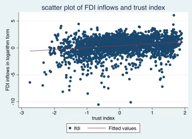
Figure 3. Scatter plot for FDI inflows (% GDP) in logarithm form and trust index

To investigate the effect of trust level on FDI inflows, I first build the trust index by using the method in section 2.3 for the period from 1984 to 2014. The upward line in Figure 3 illustrates the positive correlation between the trust index and FDI inflows (ln (FDI/GDP)) for 139 countries over the period 1984-2014. This correlation implies that a high level of trust in host country is more attractive for foreign investors. Additionally, the casual relationship between trust and FDI inflows is empirically tested by the following model:

ln ((%&'

(&))+,-) = /0+ /23+,-42+ /56+,-+ a+ + 8+- (3)

where FDI is the FDI net inflows, and T represents trust level. In this model, the first lag of the trust index is applied. X captures a vector of control variables such as school enrolment, trade rate and growth rate. Item a+ captures the unobserved effects. The

-1

0

-5

0

5

F

D

I

in

flo

w

s

in

l

o

g

a

ri

th

m

fo

rm

-3 -2 -1 0 1 2

trust index

lfdi Fitted values

25

idiosyncratic error term is 8_+-, and it should be uncorrelated with each explanatory variable across all time periods, namely, E 8_+- 6₊, :₊ = 0. Also 8_+- are homoscedastic and serially uncorrelated with Var 8+- 6+, :+ = >:? 8+- = @A5 and

Cov 8+-, 8+E 6+, :+ = 0, for all t=1, …, T and t ≠ s. The FDI data and all the controls

are collected from the World Bank’s World Development Indicators.

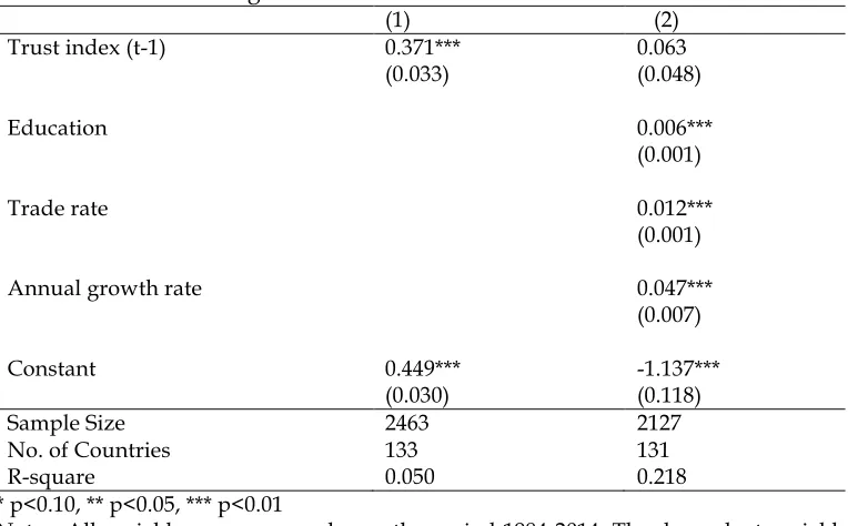
Table 7 presents the estimation results between FDI and trust by applying the pooled OLS regression method. In model (1), the trust index is positively associated with FDI at 1% significant level. The coefficient of the trust index becomes insignificant but remains positive after controlling for education, trade rate and other determinants of FDI in model (2).

Table 7. Pooled OLS regression between trust and FDI inflows

(1) (2)

Trust index (t-1) 0.371*** 0.063

(0.033) (0.048)

Education 0.006***

(0.001)

Trade rate 0.012***

(0.001)

Annual growth rate 0.047***

(0.007)

Constant 0.449*** -1.137***

(0.030) (0.118)

Sample Size No. of Countries R-square

2463 133 0.050

2127 131 0.218 * p<0.10, ** p<0.05, *** p<0.01

Notes: All variables are measured over the period 1984-2014. The dependent variable is FDI inflows measured as FDI net inflows (% of GDP). The trust index is the one built using FA. Education is measured as secondary school enrolment (% gross); the trade rate is measured as trade (% of GDP); and the annual growth rate is measured as GDP growth (annual %).

26

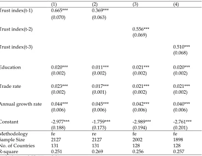
results are shown in Table 8; both random and fixed effects reveal that economies with high trust levels result in positive FDI inflows.

Table 8. Fixed effects and random effects model between trust and FDI inflow

(1) (2) (3) (4)

Trust index(t-1) 0.665*** 0.369*** (0.070) (0.063)

Trust index(t-2) 0.556***

(0.069)

Trust index(t-3) 0.510***

(0.068)

Education 0.020*** 0.011*** 0.021*** 0.020***

(0.002) (0.002) (0.002) (0.002)

Trade rate 0.023*** 0.017*** 0.021*** 0.021***

(0.002) (0.001) (0.002) (0.002)

Annual growth rate 0.044*** 0.045*** 0.042*** 0.040***

(0.006) (0.006) (0.006) (0.006)

Constant -2.977*** -1.759*** -2.989*** -2.761***

(0.188) (0.173) (0.194) (0.201)

Methodology fe re fe fe

Sample Size No. of Countries R-square

2127 131 0.251

2127 131 0.269

2002 128 0.256

1898 128 0.257 * p<0.10, ** p<0.05, *** p<0.01

Notes: All variables are measured over the period 1984-2014. The dependent variable is FDI inflows measured as FDI net inflows (% of GDP). The trust index is the one built using FA. Education is measured as secondary school enrolment (% gross); the trade rate is measured as trade (% of GDP); and the annual growth rate is measured as GDP growth (annual %). The unobserved effect a+ is assumed to

be uncorrelated with each control variable in all periods under the random regression model.

According to the Hausman test (see Appendix 5), the fixed effects model is more efficient. Based on the estimation results of fixed effects model (1), a one standard deviation increase in the trust index (t-1) would lead to a 63.8% increase in the rate of FDI inflows (%GDP). Model (1) in Table 8 also reveals that education level, trade rate and growth rate positively contribute to FDI inflows, which is consistent with the previous literature. In models (3) and (4), I further explore how historical trust levels influence current FDI inflows by using a fixed effects model. Both models uncover the important role played by the historical trust level.

27

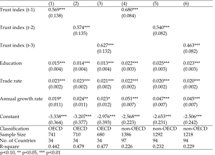
for these two groups of countries. Table 9 illustrates the estimation results between FDI and different historical levels of the trust index by applying a fixed effects model. As shown in Table 9, the coefficients of trust are all positive and significant for OECD and non-OECD countries. Therefore, trust is an important determinant of FDI for both OECD and non-OECD countries.

Table 9. Fixed effects estimations between trust and FDI inflow for OECD and non-OECD countries

(1) (2) (3) (4) (5) (6)

Trust index (t-1) 0.569*** 0.680***

(0.138) (0.084)

Trust index (t-2) 0.574*** 0.540***

(0.135) (0.082)

Trust index (t-3) 0.627*** 0.463***

(0.132) (0.082)

Education 0.015*** 0.014*** 0.013*** 0.022*** 0.025*** 0.023*** (0.004) (0.004) (0.004) (0.003) (0.003) (0.003)

Trade rate 0.023*** 0.023*** 0.021*** 0.022*** 0.020*** 0.020*** (0.002) (0.002) (0.002) (0.002) (0.002) (0.002)

Annual growth rate 0.019* 0.024** 0.023* 0.051*** 0.047*** 0.045*** (0.011) (0.011) (0.012) (0.007) (0.007) (0.007)

Constant -3.338*** -3.207*** -2.976*** -2.568*** -2.653*** -2.506*** (0.364) (0.377) (0.393) (0.223) (0.231) (0.242) Classification OECD OECD OECD non-OECD non-OECD non-OECD Sample Size

No. of Countries R-square 741 34 0.442 710 34 0.479 680 34 0.477 1386 97 0.226 1292 94 0.232 1218 94 0.229 * p<0.10, ** p<0.05, *** p<0.01

Notes: All variables are measured over the period 1984-2014. The dependent variable is FDI inflows measured as FDI net inflows (% of GDP). The trust index is the one built using FA. Education is measured as secondary school enrolment (% gross); the trade rate is measured as trade (% of GDP); and the annual growth rate is measured as GDP growth (annual %).

4.2 Trust and income inequality

28

of social trust. Since inequality might make people feel unfairly treated and exploited, social trust would decline as inequality increases.

Figure 4. Scatter plot for Gini coefficient and trust index

As shown in Figure 4, income inequality (the Gini coefficient) and the trust index (built in section 4.1) are negatively correlated for 104 countries over the period from 1984 to 2014. High trust countries are associated with low income inequality (a lower Gini coefficient). However, countries with a low level of trust are generally related to high income inequality (a higher Gini coefficient). The effect of income inequality on generalised trust has been empirically studied by Rothstein and Uslaner (2005) and Jordahl (2007). However, the influence of generalised trust on income inequality is seldom investigated5_.

To examine the influence of trust on the Gini coefficient, I employ the following econometric model:

ln IJKJ_+,- = /₀+ /₂3_+,-42+ /₅6_+,- + :₊ + L_+,- (4)

5 _{Algan and Cahuc (2013) illustrate the only cross-country study addressing how trust influences income inequality} by employing the pooled OLS regression model.

20

40

60

80

GINI

-3 -2 -1 0 1 2

Trust index

GINI coefficient Fitted values

29

where IJKJ_+,- represents the Gini coefficient for country i at time t. A high value for the Gini coefficient corresponds to a high level of income inequality in the country. Again, T refers to trust and is the same index developed in section 4.1. X captures a panel of explanatory variables including education level, income level, trade rate, inflation rate and government cost. The unobserved item is a₊. The idiosyncratic error term is L_+- and should be uncorrelated with each explanatory variable across all time periods, namely, E L_+- 6₊, :₊ = 0. Also L_+- is homoscedastic and serially uncorrelated with Var L_+- 6₊, :₊ = >:? L_+- = @_M5 and Cov L_+-, L_+E 6₊, :₊ = 0 for all t=1, …, T and

t ≠ s. The Gini coefficient and all the control variable data are collected from the World Bank’s World Development Indicators.

At first, I ignore all the endogeneity problems and adopt the pooled OLS regression method. Models (1) and (2) in Table 10 show the robust negative correlation between the trust index and the Gini coefficient. The Gini coefficient would decrease approximately 13.1% from a one standard deviation increase in one period lag of the trust index. By controlling other determinants of income inequality, the effect of the trust level decreases; a one standard deviation increase in the historical trust level leads to a 10% decrease in income inequality.

30

Table 10. Pooled OLS regression between Gini and trust

(1) (2)

Trust index (t-1) -0.137*** -0.105**

(0.026) (0.045)

Education -0.002*

(0.001)

Income 0.053

(0.042)

Trade rate

Inflation rate

-0.001 (0.001)

-0.0001 (0.000)

Government cost -0.010*

(0.005)

Constant 3.665*** 3.574***

(0.026) (0.345)

Sample Size 696 553

No. of Countries 103 95

R-square 0.187 0.292

* p<0.10, ** p<0.05, *** p<0.01

Notes: All variables are measured over the period 1984-2014. The dependent variable is GINI coefficients. The trust index is the one built using FA. Education measured as secondary school enrolment (% gross). Income is measured as the logarithm form of GDP per capita. The trade rate is measured as trade (% of GDP). The inflation rate is measured as the GDP deflator (annual %). Government cost is measured as the general government’s final consumption expenditure (% of GDP).

31

Table 11. Fixed effects, random effects and between regression of Gini and trust

(1) (2) (3)

Trust index (t-1) 0.022 0.004 -0.123**

(0.021) (0.021) (0.061)

Education 0.0003 8.27e-06 -0.003*

(0.001) (0.001) (0.002)

Income -0.048 -0.057 0.062

(0.049) (0.036) (0.053)

Trade rate Inflation rate 0.0002 (0.0004) -0.00004 (0.0001) 0.0001 (0.0004) -0.00004 (0.0002) -0.0003 (0.001) -0.0002 (0.001)

Government cost 0.001 (0.003)

0.0001 (0.003)

0.003 (0.006)

Constant 4.032*** 4.151*** 3.268***

(0.430) (0.294) (0.445)

Methodology fe re be

Sample Size 553 553 553

No. of Countries R-square 95 0.04 95 0.143 95 0.251 * p<0.10, ** p<0.05, *** p<0.01

Notes: All variables are measured over the period 1984-2014. The dependent variable is GINI coefficients. The trust index is the one built using FA. Education measured as secondary school enrolment (% gross). Income is measured as the logarithm form of GDP per capita. The trade rate is measured as trade (% of GDP). The inflation rate is measured as the GDP deflator (annual %). Government cost measured as the general government’s final consumption expenditure (% of GDP). The unobserved effect a+ is assumed to be uncorrelated with each control variable in all periods under

the random regression model.

32 Table 12. Correlation between historical Gini and trust

(1) (2) (3) (4) (5) (6) (7) (8) (9) Trust index 0.022

(0.021) 0.004 (0.021) -0.123** (0.061) (t-1)

Trust index 0.006 (0.017) -0.005 (0.016) -0.129** (0.055) (t-2)

Trust index 0.003 (0.015) -0.005 (0.015) -0.085* (0.048) (t-3)

education 0.0003 0.001 0.001 8.27e-06 0.0002 0.0004 -0.003* -0.003** -0.001 (0.001) (0.001) (0.001) (0.001) (0.001) (0.001) (0.002) (0.002) (0.002)

income -0.048 -0.055 -0.047 -0.057 -0.060* -0.060* 0.062 0.074 0.016 (0.049) (0.049) (0.047) (0.036) (0.034) (0.032) (0.053) (0.049) (0.048)

Trade rate 0.0002 0.0001 1.53e-06 0.0001 0.0001 -0.0001 -0.0003 -0.001 -0.0005 (0.000) (0.000) (0.000) (0.000) (0.000) (0.000) (0.001) (0.001) (0.001)

Inflation rate -0.00004 (0.000) -0.0002*** (0.000) -0.0002*** (0.000) -0.00004 (0.000) -0.0002*** (0.000) -0.0003*** (0.000) -0.0002 (0.001) -0.0003 (0.001) -0.003* (0.001) Government cost 0.001 (0.003) -0.001 (0.003) 0.001 (0.003) 0.0001 (0.003) -0.001 (0.003) -0.001 (0.003) 0.003 (0.006) 0.005 (0.006) -0.004 (0.006)

Constant 4.032*** (0.430) 4.120*** (0.431) 4.028*** (0.419) 4.151*** (0.294) 4.187*** (0.286) 4.170*** (0.267) 3.268*** (0.445) 3.178*** (0.408) 3.714*** (0.381)

Method fe fe fe re re re be be be

N 553 541 511 553 541 511 553 541 511 No. of

countries 95 96 93 95 96 93 95 96 93 R-square 0.040 0.075 0.103 0.143 0.142 0.158 0.251 0.290 0.240 * p<0.10, ** p<0.05, *** p<0.01

Notes: All variables are measured over the period 1984-2014. The dependent variable is Gini coefficients. The trust index is the one built using FA. Education measured as secondary school enrolment (% gross). Income is measured as the logarithm form of GDP per capita. The trade rate is measured as trade (% of GDP). The inflation rate is measured as the GDP deflator (annual %). Government cost measured as the general government’s final consumption expenditure (% of GDP). The unobserved effect a+ is assumed to be uncorrelated with each control

variable in all periods under the random regression model.

33

non-OECD countries. An econometric approach will be used to explain the correlation between trust and income inequality for OECD and non-OECD groups.

Table 13. Random effect of Gini and trust for OECD and non-OECD countries

(1) (2) (3) (4) (5) (6)

Trust index (t-1) -0.065*** 0.024

(0.022) (0.024)

Trust index (t-2)

Trust index (t-3)

-0.040* (0.022) -0.040* (0.023) 0.003 (0.018) 0.002 (0.016)

Education 0.001 (0.001) 0.001 (0.001) 0.001 (0.001) -0.001 (0.001) -0.0004 (0.001) -0.0002 (0.001)

Income 0.012 0.009 0.027 -0.024 -0.029 -0.031

(0.052) (0.053) (0.051) (0.048) (0.045) (0.043)

Trade rate Inflation rate -0.001** (0.000) -0.0003 (0.001) -0.001** (0.000) -0.0004 (0.001) -0.001** (0.000) -0.001 (0.001) 0.0001 (0.000) -7.47e-06 (0.000) 0.0001 (0.000) -0.0002*** (0.000) -0.0001 (0.000) -0.0002*** (0.000)

Government cost -0.019*** (0.004) -0.019*** (0.004) -0.019*** (0.004) 0.007** (0.003) 0.006* (0.003) 0.006* (0.004)

Constant 3.767***

(0.521) 3.791*** (0.526) 3.593*** (0.497) 3.860*** (0.390) 3.898*** (0.371) 3.908*** (0.350) Classification Sample Size OECD 196 OECD 192 OECD 186 non-OECD 357 non-OECD 349 non-OECD 325

No. of countries R-square 30 0.667 30 0.651 30 0.620 65 0.071 66 0.078 63 0.027 * p<0.10, ** p<0.05, *** p<0.01

Notes: All variables are measured over the period 1984-2014. The dependent variable is Gini coefficients. The trust index is the one built using FA. Education measured as secondary school enrolment (% gross). Income is measured as the logarithm form of GDP per capita. The trade rate is measured as trade (% of GDP). The inflation rate is measured as the GDP deflator (annual %). Government cost measured as the general government’s final consumption expenditure (% of GDP). The unobserved effect a+ is

assumed to be uncorrelated with each control variable in all periods under the random regression model.

34

with income inequality according to models (1) - (3) in Table 13. However, there is no significant effect of trust on income inequality among non-OECD countries. These results suggest that trust can effectively mitigate the income inequality issue among the OECD group. Apparently, the initial trust level is relatively high among the OECD countries, and the income inequality issue can improve as the trust level becomes stronger. However, the income inequality problem cannot be alleviated in non-OECD countries, as the improvement of trust level could be due to idiosyncratic conditions among the non-OECD countries.

5 Conclusion

The primary goal of this paper is to explore a new measure of trust. My motivation is to determine whether there is a simpler and less demanding alternative trust index for the purpose of ranking countries and exploring the effects of trust on economic performance. The current measures of trust are mainly produced by trust survey questionnaires and experimental results from trust games. However, because of the aforementioned limitations arising from ambiguous trust results obtained from trust surveys and experiments, an inter-temporal and cross-country analysis on trust becomes extremely difficult.

The trust index is constructed using the FA technique in order to assign weights to all the various characteristics that are generally considered to be determinants of generalised trust, which include the following: (i) the level of corruption and bureaucratic quality, (ii) law and order, (iii) investment profile, (iv) religious and/or ethnic tensions, (v) socioeconomic conditions, (vi) internal conflict, and (vii) secondary school enrolment. Compared to the trust survey measure, the ranking of countries in the trust index is more consistent with people’s perception.

This paper also contributes to the literature by adding the panel data study of the effects of trust on both FDI and income inequality. As a result, trust is revealed to play a significantly positive role in FDI for both OECD and non-OECD countries by employing the fixed effects model. With regard to income inequality, the random regression models show that trust is more pronounced among the OECD countries.

35

36

Appendix

Appendix 1. Summary of the components for trust index

Variable Obs Mean Std. Dev Min Max

Bureaucracy quality 3226 2.1322 1.2015 0 4

Law and order 3226 3.6556 1.5052 0 6

Corruption 3226 3.0498 1.3788 0 6

Investment profile 3226 7.0856 2.5294 0 12

Ethnic tensions 3226 3.9411 1.4719 0 6

Religious tensions 3226 4.5717 1.3630 0 6

Internal conflict 3226 8.7349 2.6904 0 12

Socioeconomic conditions 3226 5.6786 2.2441 0 11

School enrolment 2538 71.1580 31.7898 0 160.619

Appendix 2. List of average Trust Index ranking and Trust Survey ranking

Country

Trust Index

ranking Country

Trust Survey ranking

Finland 1 Norway 1

Netherlands 2 Sweden 2

Luxembourg 3 Denmark 3

Denmark 4 Finland 4

Sweden 5 China 5

Norway 6 Saudi Arabia 6

Switzerland 7 Netherlands 7

Australia 8 New Zealand 8

Iceland 9 Viet Nam 9

New Zealand 10 Switzerland 10

Austria 11 Indonesia 11

Canada 12 Canada 12

United States 13 Iraq 13

Japan 14 Australia 14

Germany 15 Japan 15

United Kingdom 16 Iceland 16

Ireland 17 Ireland 17

Belgium 18 Thailand 18

Brunei 19 Northern Ireland 19

France 20 United States 20

37

Hong Kong SAR China 22 Great Britain 22

Czech Republic 23 India 23

Hungary 24 Germany 24

Slovenia 25 Iran 25

Italy 26 Austria 26

Spain 27 Spain 27

Slovak Republic 28 Republic of Korea 28

Korea 29 Belgium 29

Cyprus 30 Italy 30

Malta 31 Germany West 31

Croatia 32 Taiwan 32

The Bahamas 33 Ukraine 33

Estonia 34 Jordan 34

Latvia 35 Belarus 35

Greece 36 South Korea 36

Poland 37 Egypt 37

Lithuania 38 Pakistan 38

Chile 39 Serbia and Montenegro 39

Namibia 40 Russian Federation 40

Botswana 41 Bulgaria 41

Bulgaria 42 Hungary 42

Saudi Arabia 43 Czech Republic 43

Oman 44 Dominican Republic 44

Kazakhstan 45 Luxembourg 45

Malaysia 46 Lithuania 46

Costa Rica 47 Mexico 47

Bahrain 48 Albania 48

Qatar 49 Uruguay 49

Kuwait 50 Armenia 50

China 51 Ethiopia 51

Argentina 52 Estonia 52

Cuba 53 Greece 53

Israel 54 Israel 54

Thailand 55 Poland 55

Tunisia 56 Bangladesh 56

Mongolia 57 Nigeria 57

Azerbaijan 58 France 58

Mexico 59 Bosnia and Herzegovina 59

Uruguay 60 Croatia 60

Belarus 61 Malta 61

Brazil 62 Slovakia 62

Moldova 63 Latvia 63

Romania 64 Azerbaijan 64

Côte d’ivoire 65 Chile 65

Morocco 66 Andorra 66

38

South Africa 68 Argentina 68

Jordan 69 South Africa 69

Trinidad and Tobago 70 Georgia 70

Bolivia 71 Republic of Moldova 71

Albania 72 Slovenia 72

Libya 73 Moldova 73

United Arab Emirates 74 Mali 74

Syrian Arab Republic 75 Singapore 75

Jamaica 76 Romania 76

Vietnam 77 Kyrgyzstan 77

Ecuador 78 Portugal 78

Dominican Republic 79 Guatemala 79

Iran 80 Serbia 80

Gabon 81 Venezuela 81

Russia 82 Burkina Faso 82

Lebanon 83 El Salvador 83

Venezuela 84 Puerto Rico 84

The Gambia 85 Colombia 85

Turkey 86 Zimbabwe 86

Armenia 87 Zambia 87

Egypt 88 Turkey 88

Papua New Guinea 89 Algeria 89

India 90 Macedonia, Republic of 90

Panama 91 Cyprus 91

Madagascar 92 Malaysia 92

Paraguay 93 Ghana 93

Ghana 94 Tanzania, United Republic Of 94

Colombia 95 Uganda 95

Burkina Faso 96 Peru 96

Zimbabwe 97 Philippines 97

El Salvador 98 Brazil 98

Philippines 99 Rwanda 99

Nicaragua 100 Trinidad and Tobago 100

Kenya 101

Malawi 102

Senegal 103

Peru 104

Tanzania 105

Guyana 106

Algeria 107

Suriname 108

39

Congo 110

Guatemala 111

Cameroon 112

Yemen 113

Indonesia 114

Mozambique 115

Guinea 116

Honduras 117

Zambia 118

Togo 119

Mali 120

Uganda 121

Ethiopia 122

Niger 123

Guinea-Bissau 124

Pakistan 125

Angola 126

Myanmar 127

Sri Lanka 128

Sudan 129

Bangladesh 130

Nigeria 131

Somalia 132

Liberia 133

Iraq 134

Haiti 135

40

Appendix 3. Comparison of average Trust Index ranking and Trust Survey ranking

Country Trust index ranking Trust survey ranking

Finland 1 4

Netherlands 2 7

Luxembourg 3 40

Denmark 4 3

Sweden 5 2

Norway 6 1

Switzerland 7 10

Australia 8 14

Iceland 9 16

New Zealand 10 8

Austria 11 25

Canada 12 12

United States 13 19

Japan 14 15

Germany 15 23

United Kingdom 16 21

Ireland 17 17

Belgium 18 27

France 19 53

Portugal 20 67

Hong Kong SAR China 21 20

Czech Republic 22 38

Hungary 23 37

Slovenia 24 63

Italy 25 28

Spain 26 26

Slovak Republic 27 56

Korea 28 32

Cyprus 29 77

Malta 30 55

Croatia 31 54

Estonia 32 47

Latvia 33 57

Greece 34 48

Poland 35 50

Lithuania 36 41

Chile 37 59

Bulgaria 38 36

Saudi Arabia 39 6

Malaysia 40 78

41

Argentina 42 61

Israel 43 49

Thailand 44 18

Azerbaijan 45 58

Mexico 46 42

Uruguay 47 44

Belarus 48 31

Brazil 49 84

Moldova 50 64

Romania 51 66

Morocco 52 60

Ukraine 53 29

South Africa 54 62

Jordan 55 30

Trinidad and Tobago 56 85

Albania 57 43

Vietnam 58 9

Dominican Republic 59 39

Iran 60 24

Russia 61 35

Venezuela 62 69

Turkey 63 75

Armenia 64 45

Egypt 65 33

India 66 22

Ghana 67 79

Colombia 68 72

Burkina Faso 69 70

Zimbabwe 70 73

El Salvador 71 71

Philippines 72 83

Peru 73 82

Tanzania 74 80

Algeria 75 76

Guatemala 76 68

Indonesia 77 11

Zambia 78 74

Mali 79 65

Uganda 80 81

Ethiopia 81 46

Pakistan 82 34

Bangladesh 83 51

Nigeria 84 52

42 Appendix 4. Sample statistic

Full sample (139) OECD Countries (31) Non-OECD Countries (108)

Variable Obs Mean Std. Obs Mean Std. Obs Mean Std.

Dev. Dev. Dev.

trust index(a) 2,383 1.18E-09 0.9582 - - - - 0.8822(be)

0.3709(wi)

trust index(b) 2,823 -6.50E-10 0.9569 877 0.9765 0.6015 1,946 -0.4401 0.736 0.8873(be)

0.3593(wi)

0.5499(be) 0.2496(wi)

0.6477 0.3990 L1.trust

index(b) 2,820 0.0006 0.9570 877 0.9765 0.6015 1,943 -0.4398 0.7362 0.8879(be)

0.3593(wi)

0.5499(be) 0.2496(wi)

0.6482(be) 0.3992(wi) L2.trust

index(b) 2,787 0.0064 0.9591 877 0.9765 0.6015 1,910 -0.439 0.7386 0.8875(be)

0.3598(wi)

0.5499(be) 0.2496(wi)

0.6491(be) 0.4005(wi) L3.trust

index(b) 2,692 0.0049 0.9625 844 0.9807 0.6035 1,848 -0.4408 0.7413 0.8894(be)

0.3636(wi)

0.5511(be) 0.2513(wi)

0.6505(be) 0.4048(wi)

lfdi 3,436 0.4566 1.5986 869 0.525 1.3519 2,567 0.4334 1.6734

lgini 938 3.6677 0.2664 252 3.4872 0.2204 686 3.734 0.2507

income 3,133 9.0981 1.265 803 10.2643 0.4569 2,330 8.6962 1.2039

education 2,978 72.9668 31.3267 927 99.0027 15.4272 2,051 61.1992 29.5389

trade rate 3,778 79.1374 51.801 965 79.9813 46.8815 2,813 78.8479 53.3891

inflation rate 3,893 53.5259 587.2015 965 8.2336 36.0034 2,928 68.4532 676.1347 government

cost 3,881 15.9548 6.2429 996 18.74 4.3814 2,885 14.9932 6.4967

43 Appendix 5. Hausman test

---- Coefficients ---- (b) (B) fe re

(b-B) Difference

sqrt(diag(V_b-V_B)) S.E.

Trust index(t-1) 0.6650 0.3693 0.2957 0.0313

Education 0.0197 0.0111 0.0086

0.0014

Trade rate 0.0227 0.0168 0.0059 0.0011

Annual growth rate

0.0445 0.0449 -0.0004 0.0008

b= consistent under N0 and NO; obtained from xtreg

B= inconsistent under NO, efficient under N0; obtained from xtreg

Test: N0: difference in coefficients not systematic

Chi2(4) = (b-B)’[(V_b-V_B)^(-1)](b-B) = 197.54

44 Appendix 6.

20

30

40

50

60

GINI

-2 -1 0 1 2

Trust index

GINI coefficient Fitted values

scatter plot for GINI coefficients and trust index for OECD countries

20

40

60

80

GINI

-3 -2 -1 0 1 2

Trust index

GINI coefficient Fitted values

45 Appendix 7. Hausman test

---- Coefficients ---- (b) (B) fe re

(b-B) Difference

sqrt(diag(V_b-V_B)) S.E.

Trust index(t-1) 0.0217 0.0042 0.0175 0.0049

Education 0.0003 8.27e-06 0.0002

0.0001

Income -0.0476 -0.0572 0.0096 0.0135

Trade rate 0.0002 0.0001 0.0001 0.0001

Inflation rate -0.00003 -0.00004 -4.54e-07 0.00001

Government consumption

0.0014 0.0001 0.0013 0.0011

b= consistent under N0 and NO; obtained from xtreg

B= inconsistent under NO, efficient under N0; obtained from xtreg

Test: N0: difference in coefficients not systematic

Chi2(6) = (b-B)’[(V_b-V_B)^(-1)](b-B) = 18.81

46

Reference

1. Abramson, P. R., and Inglehart, R. 1995. Value change in global perspective. Ann

Arbor: University of Michigan Press.

2. Aghion, P., Algan, Y., Cahuc, P., and Shleifer, A. 2010. Regulation and distrust. The

Quarterly Journal of Economics, 125, 1015-1049.

3. Alesina A., Baqir, R., and Easterley, W. 1999. Public goods and ethnic divisions. The

Quarterly Journal of Economics, 114 (4), 1243-1284.

4. Alesina, A., and La Ferrara, E. 2000. Participation in heterogeneous communities. The

Quarterly Journal of Economics, 115 (3), 847-904.

5. Alesina, A., and La Ferrara, E. 2002. Who trust others? Journal of Public Economics, 85

(2), 207-234.

6. Algan, Y., and Cahuc, P. 2009. Civic virtue and labor market institutions. American

Economic Journal: Macroeconomics, 1(1), 111-145.

7. Algan, Y., and Cahuc, P. 2013. Trust, growth and well-being: new evidence and policy

implications. IZA Discussion Papers 7464, Institute for the Study of Labor (IZA).

8. Arrow, Kenneth J. 1972. Gifts and Exchanges. Philosophy and Public Affairs, 1, 343-367.

9. Baliamoune-Lutz, M. 2009. Human well-being effects of institutions and social capital.

Contemporary Economic Policy, 27 (1), 54-66.

10. Baliamoune-Lutz, M. 2011. Do institutions and social cohesion enhance the

effectiveness of aid? New Evidence from Africa. ICER Working Papers 13-2011.

11. Banfield, E. 1958. The Moral Basis of a Backward Society. New York: Free Press.

12. Bhardwaj, A., Dietz, J., and Beamish, P.W. 2007. Host country cultural influences on

foreign direct investment. Management International Review, 47 (1), 29–50.

13. Berg, J., Dickhaut, J., and McCabe, K. 1995. Trust, reciprocity and social history. Games

and Economic Behavior, 10, 122-42.

14. Berggren, N., Elinder, M. and Jordahl, H. 2008. Trust and growth: A shaky

relationship. Empirical Economics, 35 (2), 251-274.

15. Beugelsdijk, S., De Groot, H.L. F., and Van Schaik, A.B.T.M. 2004. Trust and economic