Forecasting with Temporal Hierarchies

Munich Personal RePEc Archive

Forecasting with Temporal Hierarchies

Athanasopoulos, George and Hyndman, Rob J. and

Kourentzes, Nikolaos and Petropoulos, Fotios

28 August 2015

Online at

https://mpra.ub.uni-muenchen.de/66362/

Please cite this paper as:

Athanasopoulos, A et al (2015) “Forecasting with Temporal Hierarchies”, Lancaster University

Management School, Working Paper series, Working Paper 2015:3

Lancaster University Management School

Working Paper 2015:3

Forecasting with Temporal Hierarchies

George Athanasopoulos, Rob J. Hyndman, Nikolaos

Kourentzes, Fotios Petropoulos

The Department of Management Science

Lancaster University Management School

Lancaster LA1 4YX

UK

© George Athanasopoulos, Rob J. Hyndman, Nikolaos Kourentzes, Fotios Petropoulos All rights reserved. Short sections of text, not to exceed

two paragraphs, may be quoted without explicit permission, provided that full acknowledgment is given.

Forecasting with Temporal Hierarchies

George Athanasopoulosa, Rob J. Hyndmana, Nikolaos Kourentzesb,∗, Fotios Petropoulosc

a

Department of Econometrics and Business Statistics Monash University, Australia

b

Lancaster University Management School Department of Management Science, UK

c

Logistics and Operations Management Section Cardiff Business School, UK

Abstract

This paper introduces the concept of Temporal Hierarchies for time series forecasting. A tem-poral hierarchy can be constructed for any time series by means of non-overlapping temtem-poral aggregation. Predictions constructed at all aggregation levels are combined with the proposed framework to result in temporally reconciled, accurate and robust forecasts. The implied com-bination mitigates modelling uncertainty, while the reconciled nature of the forecasts results in a unified prediction that supports aligned decisions at different planning horizons: from short-term operational up to long-short-term strategic planning. The proposed methodology is independent of forecasting models. It can embed high level managerial forecasts that incorporate complex and unstructured information with lower level statistical forecasts. Our results show that fore-casting with temporal hierarchies increases accuracy over conventional forefore-casting, particularly under increased modelling uncertainty. We discuss organisational implications of the temporally reconciled forecasts using a case study of Accident & Emergency departments.

Keywords: Hierarchical forecasting, temporal aggregation, reconciliation, forecast combination

JEL: C44, C53

1. Introduction

Decision making at the operational, tactical and strategic level is at the core of any organ-isation. Forecasts that support such decisions are inherently different in nature. For example, strategic decisions require long-run forecasts at an aggregate level, while decisions at the highly dynamic operational level require short-term very detailed forecasts. The differences in time granularity affects how these forecasts are generated. Long-run strategic forecasts are usu-ally generated considering high level unstructured information from the business environment. These primarily rely on the skill, judgement and experience of senior management, as accurate long-term statistical forecasts that capture the market dynamics can be very challenging to produce (Kolsarici and Vakratsas, 2015). In contrast short-run operational forecasts are usually generated using structured but limited sources of information, such as past sales. These mostly rely on statistical methods. Furthermore even within the same decision-making level, it is well known in the forecasting literature that different forecast horizons require different methods.

∗_{Correspondance: N Kourentzes, Department of Management Science, Lancaster University Management}

Since these forecasts are produced by different approaches and are based on different infor-mation sets, it is expected that they may not agree. This disagreement can lead to decisions that are not aligned. For example the day-to-day operational forecasts of a manufacturer that support inventory and production decisions may provide an overall stable view of the market. In contrast the forecasts at the strategic level may predict a booming market, with various implications for the investment strategy and budgetary decisions. For that company to be able to meet its growth potential all operational, tactical and strategic forecasts and in turn deci-sions must be aligned. Otherwise this misalignment can lead to waste or lost opportunities, and additional costs.

Naturally there are various processes that attempt to align managerial decisions. A mini-mum requirement for this to be achieved is that forecasts supporting these decisions must be reconciled; i.e., lower level forecasts must add up to higher level forecasts resulting in consis-tent forecasts. It is often the case that within organisations this reconciliation of forecasts, and especially the alignment of decision making, is done in a top-down manner, with variable success. The ideal solution however would be to somehow combine the most accurate aspects of the forecasts from each level, thereby avoiding a myopic view from a single level. To achieve consistent forecasts that support all decisions from operational to strategic, the reconciliation must be done at different data frequencies and different forecast horizons.

The contribution of this paper is to introduce a novel approach for time series modelling

and forecasting: Temporal Hierarchies. Consider a time series observed at some sampling

fre-quency. Using aggregation of non-overlapping observations we construct several aggregate series of different frequencies up to the annual level. We define as a temporal hierarchy the structural connection across the levels of aggregation. Each level highlights different features of the time series, resulting in independent forecasts that contain different information. As we argue above, the forecasts at different aggregation levels can support different managerial decisions and may not be reconciled. Making use of the temporal hierarchy structure we optimally combine the forecasts from all levels of aggregation, merging the different views of the data. This leads to: (a) reconciled forecasts, supporting better decisions across planning horizons; (b) increased forecast accuracy; and (c) mitigating modelling risks. These are achieved without needing any additional inputs to conventional forecasting.

We develop the theoretical framework of temporal hierarchies and empirically demonstrate using real and simulated data their benefits under parameter and model uncertainty, resulting in forecast accuracy gains. Finally we demonstrate their use in a case study of Accident & Emergency departments, by reconciling forecasts that support operational, tactical and strategic decisions, while at the same time obtaining substantial gains in accuracy.

The paper is structured as follows: Section 2 summarises findings from temporal aggregation and hierarchical forecasting, which are necessary for the development of temporal hierarchies; Section 3 introduces the notion of temporal hierarchies and Section 4 presents the theoretical framework for forecasting, which is empirically evaluated in a large dataset of real time series in Section 5. Section 6 explores the conditions under which temporal hierarchies offer benefits over conventional time series modelling using simulations. Finally Section 7 demonstrates their use and benefits in a case study of Accident & Emergency departments, followed by concluding remarks.

2. Background

When temporal aggregation is applied to a time series it can strengthen or attenuate differ-ent elemdiffer-ents. Non-overlapping temporal aggregation is a filter of high frequency compondiffer-ents,

therefore at an aggregate view low frequency components, such as trend/cycle, will dominate. The opposite is true for disaggregate data, where potential seasonality may be visible. There-fore, temporal aggregation can be seen as a tool to better understand and model the data in hand.

Temporal aggregation is not a new topic. Studying its effects on univariate time series models goes back to the seminal work of Amemiya and Wu (1972), Tiao (1972) and Brewer (1973). The theoretical results on ARIMA processes from these papers are summarised by Rossana and Seater (1995) as being threefold: (a) temporal aggregation contaminates/complicates the

dynamics of the underlying ARIMA(p, d, q) process through the moving average component

(they refer to this as the Brewer effect); (b) as the level of aggregation increases the process at the aggregate level is simplified and converges to an IMA(d, d) (they call this the Tiao effect); and (c) aggregation causes loss in the number of observations resulting in a loss in estimation efficiency (they call this the sample size effect). Wei (1979) was first to study the effect of temporal aggregation on seasonal ARIMA processes. His theoretical findings are in line with the summary by Rossana and Seater (1995).

Rossana and Seater (1995) also study the end result of the above effects on several key macroeconomic variables and conclude that temporal aggregation to the annual level greatly simplifies the complex low-frequency cyclical ARIMA dynamics found in monthly and quarterly data. This results in each of these variables being adequately modelled by a random walk process or an IMA(1,1) at the annual level. They state that “quarterly data may be the best compromise among frequency of observation, measurement error, and temporal aggregation distortion”. A similar conclusion is reached by Nijman and Palm (1990).

Hotta and Cardoso Neto (1993) show that the loss in forecast efficiency using aggregated data is not large, even when the underlying model is unknown. Thus, prediction could be done by either disaggregated or aggregated models. They give two reasons for when temporal aggregation may be a good idea in practice: (a) in some circumstances the aggregate series may be better represented by a linear model than the disaggregate series; and (b) the aggregate series is less affected by outliers compared to the disaggregate series. Hotta (1993) also finds that an additive outlier can have a stronger effect on the disaggregate model than the aggregate.

Both Silvestrini et al. (2008) and Abraham (1982) provide empirical evidence of cast accuracy gains from forecasting with the aggregate model rather than aggregating fore-casts from the disaggregate model. Souza and Smith (2004) use simulations to find that for ARFIMA(p, d, q) processes withd <0, forecasts from the aggregated series are generally supe-rior than aggregated forecasts from the disaggregate series, while the results are reversed for d >0 but the evidence is not as clear.

Rostami-Tabar et al. (2013) look into identifying an optimal aggregation level when the disaggregate process is either MA(1) or AR(1) and find that in general the higher the aggregation the lower the forecast errors are, when forecasting by single exponential smoothing. For more complex processes Nikolopoulos et al. (2011) demonstrate that forecasting accuracy does not change monotonically as the aggregation level increases.

forecast accuracy using multiple aggregation levels while overcoming the need to select a single (optimal) level.

The temporal hierarchies we introduce in this paper specify the connection between an observed and temporally aggregated time series. This has analogies with the cross-sectional dimension where there are time series connected by a hierarchical structure. This is referred to as “hierarchical time series” and forecasts are required for each of these series (Fliedner, 2001). Consider for example a manufacturer that requires forecasts for total production for purchasing raw materials, but also forecasts at the very disaggregate level for inventory management of finished products. Obviously these hierarchies can have several levels.

Traditionally either the top-down or the bottom-up approaches are used to produce forecasts for the hierarchy. According to the former forecasts are generated for the time series at the top level and then disaggregated down all the way to the bottom level, while for the latter forecasts are generated at the very bottom level and then aggregated up. Such approaches ensure that forecasts add up across the hierarchy.

The advantages and disadvantages of these traditional approaches are not complementary. The top-down approach requires forecasts for only one time series at the very aggregate level. However aggregation implies a large loss of information and it is challenging to disaggregate the forecasts down the hierarchy (see Gross and Sohl 1990 and Athanasopoulos et al. 2009 for a summary of top-down approaches). In contrast bottom-up implies no loss of information but it requires many and possibly very noisy time series to be forecast. A compromising alternative is the “middle-out ” approach where forecasts are generated at some intermediate aggregation level, and aggregated and disaggregated appropriately.

One aspect that becomes immediately obvious is that the time series at a single level of aggregation where the forecasts are created will dominate the generation of forecasts, ignoring information at all other levels. To counter this significant limitation Hyndman et al. (2011) introduced a regression based approach that instead optimally combines forecasts from all the series of the hierarchy and results in reconciled forecasts. This method is used by Athanasopou-los et al. (2009) with good empirical results and further developed by Wickramasuriya et al. (2015). As well as achieving reconciliation, this method has been shown to result in significant forecast improvements over the traditional approaches in the cross-sectional setting.

A crucial reason for this improvement is forecast combinations. Forecast combinations are widely regarded as beneficial, leading to a reduction of forecast error variance (Bates and Granger, 1969; Makridakis and Winkler, 1983; Clemen, 1989; Timmermann, 2006). Ways to best combine forecasts have been widely investigated, resulting in various sophisticated weighting methods (see Newbold and Granger, 1974; Min and Zellner, 1993; Elliott and Timmermann, 2004, 2005); yet, simple approaches, such as the unweighted average, are found to perform as well as more sophisticated approaches (Timmermann, 2006). The literature has also focused on combining forecasts from different sources, particularly from human experts with different available information (see Ashton and Ashton, 1985; Goodwin, 2000; Lamberson and Page, 2012; Budescu and Chen, 2014). Furthermore, forecast combinations effectively limit the need for model selection (Kolassa, 2011) and reduce the uncertainty in terms of model specification and estimation (Breiman et al., 1996; Kourentzes, Barrow and Crone, 2014).

In the context of temporal aggregation, Kourentzes, Petropoulos and Trapero (2014) use unweighted combinations of forecasts from different aggregation levels, but provide evidence that weighted combinations are beneficial using ad-hoc weights. Hyndman et al. (2011) consider the analogous cross-sectional problem and derive the weights from the structure of the hierarchy. In this paper, by constructing temporal hierarchical structures we are able to apply a similar approach to temporal hierarchies.

We argue that hierarchical forecasting is a much broader notion than the cross-sectional hierarchies that are usually considered. A hierarchy can be defined either across time series, or temporally from a single time series. In the following sections we define temporal hierarchies and the forecasting framework based on them.

3. Temporal hierarchies

Suppose we observe a time series at monthly intervals. From this series, we can construct various aggregate series such as quarterly and annual series, as well as less common variations

such as series consisting of 2-month, 4-month and 6-month aggregates. In fact, any k-month

aggregate wherekis a factor of 12 is a useful variant and has seasonal period equal to 12/k. Ifk is not a factor of 12, then the seasonality of the aggregate series is non-integer, and so forecasts of the aggregate are more difficult to compute.

More generally, we are interested in a time series{yt; t= 1, . . . , T} observed at the highest

available sampling frequency per year,m, and in thek-aggregates that can be constructed where kis a factor of m. The various aggregated series can be written as

y_j[k]=

t⋆

+jk−1

X

t=t⋆_+(j−1)k

yt, (1)

for j = 1, . . . ,⌊T /k⌋ and Mk =m/k is the seasonal period of the aggregated series. The

non-overlapping aggregation requires that the total number of observations has to be a multiple of m. To ensure this, we start the aggregation from t⋆ =T− ⌊T /m⌋m+ 1.

By restricting k to factors of m, we do not introduce any non-integer seasonality (if our

observed series is seasonal). This avoids the challenge of having to model non-integer seasonality as most forecasting models require integer seasonal periods. If models capable of handling such seasonality are used this restriction is not required.

We denote the factors of m, in descending order, to be {kp, . . . , k3, k2, k1} where kp =m,

k1= 1 and p is the total number of aggregation levels. For example, for quarterly data

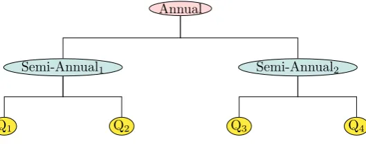
k∈ {4,2,1}, and therefore every four quarterly observations are aggregated up to annual and semi-annual observations as shown in the Figure 1.

Annual

Semi-Annual1

Q1 Q2

Semi-Annual2

Q3 Q4

Figure 1: Temporal hierarchy for quarterly series.

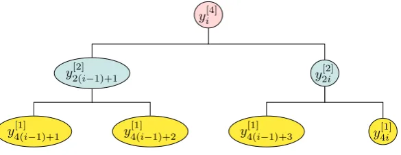
Note that the observation index j varies with each aggregation levelk. Therefore, in order

to express a common index for all levels, we define i as the observation index of the most

aggregate series, i.e. y[m]_i , so thatj=iat that level. Using (1) and indexi= 1, . . . ,⌊T /m⌋, we can express each observation at each level of aggregation as y_M[k]

k(i−1)+z, forz= 1, . . . , Mk. An

yi[4]

y₂₍[2]i₋1)+1

y₄₍[1]i₋1)+1 y [1] 4(i₋1)+2

y[2]₂i

y[1]₄₍i₋1)+3 y [1] 4i

Figure 2: Temporal hierarchy for quarterly series using the common indexifor all levels of aggregation.

andzcontrols the increase within each year. Following this notation, the quarterly hierarchical structure can be defined as in Figure 2.

We stack the observations for each aggregation level below the annual level in column vectors such that

y[k]_i = (y_M[k]

k(i−1)+1, y

[k]

Mk(i−1)+2, . . . , y

[k] Mki)

′_{. (2)}

Collecting these in one column vector,yi =

y[m]_i , . . . ,y[k3]′

i ,y [k2]′

i ,y [1]′

i

′

, we can write

yi=Sy_i[1] (3)

where for quarterly data

S =

         

1 1 1 1 1 1 0 0 0 0 1 1 1 0 0 0 0 1 0 0 0 0 1 0 0 0 0 1

         

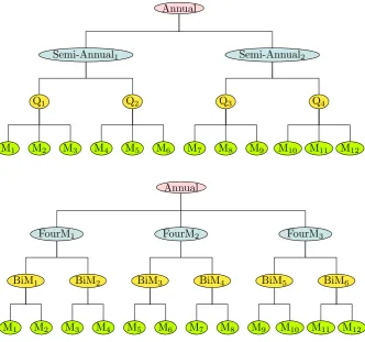
is referred to as the “summing” matrix (drawing from the work of Hyndman et al. 2011) and y[1]_i is the vector of observations of the time series observed at the highest available frequency. It is not always possible to represent the aggregated series in a single tree such as Figure 1. For monthly data, the aggregates of interest are for k ∈ {12,6,4,3,2,1}. Hence the monthly observations are aggregated to annual, semi-annual, four-monthly, quarterly and bi-monthly observations. These can be represented in two separate hierarchies, as shown in Figure 3.

Annual

Semi-Annual1

Q1

M1 M2 M3

Q2

M4 M5 M6

Semi-Annual2

Q3

M7 M8 M9

Q4

M10 M11 M12

Annual

FourM1

BiM1

M1 M2

BiM2

M3 M4

FourM2

BiM3

M5 M6

BiM4

M7 M8

FourM3

BiM5

M9 M10

BiM6

M11 M12

Figure 3: The implicit hierarchical structures for monthly series.

However, the appropriate summing matrix for monthly series is easily obtained:

S =                             

1 1 1 1 1 1 1 1 1 1 1 1

1 1 1 1 1 1 0 0 0 0 0 0

0 0 0 0 0 0 1 1 1 1 1 1

1 1 1 1 0 0 0 0 0 0 0 0

0 0 0 0 1 1 1 1 0 0 0 0

0 0 0 0 0 0 0 0 1 1 1 1

1 1 1 0 0 0 0 0 0 0 0 0

.. .

0 0 0 0 0 0 0 0 0 1 1 1

1 1 0 0 0 0 0 0 0 0 0 0

.. .

0 0 0 0 0 0 0 0 0 0 1 1

I12                              ,

and we can again write

yi=Sy_i[1] (4)

whereyi=

4. Forecasting framework

Given a temporal hierarchy, our objective is to produce forecasts. As with cross-sectional hierarchies, we can take advantage of the hierarchical structure to assist in producing better forecasts than if we simply forecast the most disaggregate time series. We impose the constraint that any forecast at an aggregate level is equal to the sum of the forecasts of the respective subaggregate forecasts from the level below, as defined by the temporal hierarchy used.

Let h∗ be the maximum required forecast horizon at the most disaggregate level available,

and therefore h = 1, . . . ,⌈h∗/m⌉ defines the forecast horizons required at the most aggregate annual level. Then for each aggregation level kwe generate a set of Mkh steps-ahead forecasts

conditional on⌊T /k⌋observations. We refer to these as base forecasts. For each forecast horizon h we stack the forecasts the same way as the data, i.e.,

ˆ

yh = (ˆy[m]h , . . . ,yˆ [k3]′

h ,yˆ [k2]′

h ,yˆ [1]′

h )′

where each ˆy[k]_h = (ˆy_M[k]

k(h−1)+1,yˆ

[k]

Mk(h−1)+2, . . . ,yˆ

[k] Mkh)

′ _{is of dimensionM}

kand therefore ˆyh is of

dimensionP

kℓ.

We can write the base forecasts as

ˆ

yh =Sβ(h) +εh (5)

where β(h) = E[y[1]_{⌊T /m⌋+h} | y1, . . . , yT] is the unknown conditional mean of the future values

of the most disaggregated observed series, and εh represents the “reconciliation error”, the

difference between the base forecasts ˆyh and their expected value if they were reconciled. We

assume that ε_h has zero mean and covariance matrix Σ. We refer to (5) as the temporal

reconciliation regression model. It is analogous to the cross-sectional hierarchical reconciliation regression model proposed by Hyndman et al. (2011) and also applied in Athanasopoulos et al. (2009) for reconciling forecasts of structures of tourism demand. A similar idea has been used for imposing aggregation constraints on time series produced by national statistical agencies (Quenneville and Fortier, 2012).

IfΣwas known, the generalised least squares (GLS) estimator ofβ(h) would lead to recon-ciled forecasts given by

˜

yh =Sβˆ(h) =S(S′Σ−1S)−1S′Σ−1yˆh =SPyˆh, (6)

which would be optimal in that the base forecasts are adjusted by the least amount (in the

sense of least squares) so that these become reconciled. In general, Σis not known and needs

to be estimated. Hyndman et al. (2011) and Athanasopoulos et al. (2009) avoid estimatingΣ

by using ordinary least squares (OLS), replacing Σby σ2I in (6). This is only optimal under

some special conditions, such as when the reconciliation errors are equivariant and uncorrelated, or when the base forecast errors satisfy the same aggregation constraints as the original data (Hyndman et al., 2011), neither of which is likely to be true. For the temporal hierarchy case the errors are not equivariant by definition.

Recently, Wickramasuriya et al. (2015) showed that Σ is not identifiable. Assuming that

the base forecasts are unbiased they show that for the forecast errors of the reconciled forecasts,

Var(y_{⌊T /m⌋+h}−y˜h) =SP W P′S′

where W = Var(y_{⌊T /m⌋+h} −yˆh) is the covariance matrix of the base forecast errors. By

minimizing the variances of the reconciled forecast errors, they propose an estimator which results in unbiased reconciled forecasts given by

˜

y_h =S(S′W−1S)−1S′W−1yˆ_h. (7)

Note that this coincides with the GLS estimator in (6) but with a different covariance matrix. Defining the in-sample one-step-ahead base forecast errors asei =

e[m]_i , . . . ,e[k3]′

i ,e [k2]′

i ,e [1]′

i

′

, fori= 1, . . . ,⌊T /m⌋, the sample covariance estimator ofW is given by,

Λ= 1

⌊T /m⌋

⌊T /m⌋

X

i=1

eie′i, (8)

which is a κ×κ matrix with κ=Pp

ℓ=1kℓ.

There are two challenges with implementing this estimator in practice. First, Λ has κ2

elements to be estimated. The sample size for each element is bound by⌊T /m⌋, the number of observations at the annual level and⌊T /m⌋ ≪T. Second, forecasting with temporal hierarchies does not require model-based forecasts and this means that in-sample forecast errors may not always be available. Consider for example the case where senior management is generating forecasts at the aggregate strategic level based on their expertise or the case where judgemental adjustment has been implemented. To overcome these challenges we propose three diagonal estimators that approximateΛ. By definition these ignore correlations across aggregation levels but allow for varying degrees of heterogeneity and lead to alternative weighted least squares (WLS) estimators. The estimators are of increasing simplicity and are easily implemented in practice. Our results show that these work well in the extensive empirical application and

simulations. An alternative would be to consider shrinkage estimators for Λ instead (see for

example Sch¨afer and Strimmer, 2005), however this does not address the second challenge

outlined above.

Hierarchy variance scaling

The first estimator, ΛH, we implement is the diagonal of Λ that has only κ elements to

be estimated. This estimator accounts for the heterogeneity across temporal aggregation levels but also within each level in the hierarchy. For example, there are two forecasts errors for each year at the semi-annual level. A different variance estimate is used to scale the contribution of the first and the second semi-annual forecasts.

Series variance scaling

Although using the diagonal of the sample covariance matrix requires fewer error variances to be estimated compared to the unrestricted covariance matrix, the sample available for estimating each variance is again limited to ⌊T /m⌋. Alternatively, since the forecast errors within the same aggregation level are for the same time series, it is not unreasonable to assume that their variances are the same. In fact this is the variance estimated in conventional time series

modelling. This will decrease the number of variances to be estimated to p, the total number

of aggregation levels and increase the sample size available for estimation by m/k per level.

Therefore under ‘series variance scaling’ we define diagonal matrixΛV which contains estimates

of the in-sample one-step-ahead error variances across each level.

Structural scaling

we set Σ=σ2_Λ

S whereΛS is a diagonal matrix with each element containing the number of

reconciliation errors contributing to that aggregation level:

ΛS = diag(S1), (9)

where 1 is a unit column vector of the dimension of ˆy_h[1] (the forecasts from the most disag-gregate level). This estimator has several desirable properties. First, it depends only on the

seasonal periodmof the most disaggregated observations, and is independent of both data and

forecasting model. Second, it permits forecasts which originate from any forecasting method or even predictions from human experts that are not described by a formal model, since no estimation of the variance of the forecast errors is needed.

To better illustrate the differences between the three proposed scaling methods we show the different matrices for quarterly data:

ΛH = diag ˆσ[4]A,σˆ [2] SA1,σˆ

[2] SA2,σˆ

[1] Q1,σˆ

[1] Q2,σˆ

[1] Q3,ˆσ

[1] Q4

2

,

ΛV = diag ˆσ[4],σˆ[2],σˆ[2],ˆσ[1],σˆ[1],σˆ[1],σˆ[1]2, ΛS = diag 4,2,2,1,1,1,1

,

where the diagonal elements of ΛH correspond to the error variances of the series that make

up the quarterly temporal hierarchy in Figure 1, and the diagonal elements ofΛV are the error

variances of each aggregation level k∈ {4,2,1}. The increasing simplicity of each scaling is evident.

In the empirical section that follows we report the results using each of the three scaling methods for WLS.

5. Empirical evaluation

5.1. Experimental setup

We perform an extensive empirical evaluation of forecasting with temporal hierarchies using the 1,428 monthly and 756 quarterly time series from the M3 competition (Makridakis and Hibon, 2000). In order to ensure the comparability of our results with the original competition, we withhold as test samples the last 18 observations of each monthly series and the last 8 observations of each quarterly series.

We construct temporal hierarchies, as proposed in Section 3, by aggregating the monthly series to bi-monthly, quarterly, four-monthly, semi-annual and annual levels, and the quar-terly series to semi-annual and annual levels. For each series at each aggregation level we independently generate base forecasts over the test samples using the automated algorithms for ExponenTial Smoothing (ETS) and AutoRegressive Integrated Moving Average (ARIMA)

models as implemented in theforecast package for R (Hyndman, 2015; R Core Team, 2012) and

described in Hyndman and Khandakar (2008). These are labelled as ‘Base’ in the tables that follow.

Our aim in what follows is to evaluate the forecast accuracy of reconciled forecasts generated from forecasting with temporal hierarchies which have as input the base forecasts and demon-strate any gains in performance due to using temporal hierarchies. As it is quite common for organisations to require forecasts at different horizons for different purposes, the base forecasts for each level form a natural benchmark. For example, short-term operational, medium-term tactical and long-term strategic forecasts are often required at the monthly, quarterly and annual levels respectively. The base forecasts are the best an organisation can do at each aggregation

level. However these base forecasts are without the additional and important property of being reconciled, and they do not take advantage of the information available at the other temporal aggregation levels. In the evaluation that follows, a desirable result would be that the recon-ciled forecasts are no less accurate than the base forecasts. In presenting the results, as we are not able to exactly aggregate the 18 observations of the monthly test samples to annual and four-monthly observations, we aggregate only the first 12 observations of each test sample to one annual observation and the first 16 observations to 4 four-monthly observations which we then use for evaluation.

The first set of reconciled forecasts comes from applying the bottom-up method. In this method, all reconciled forecasts are constructed as temporal aggregates of the lowest level

forecasts (for k = 1). The inclusion of the bottom-up method is motivated by the literature

on temporal aggregation which argues that estimation efficiency is lost due to aggregation and therefore there are limited benefits to be had by modelling time series at temporally aggregated levels (see Section 2). The bottom-up forecasts form a natural benchmark in order to assess the benefits of generating forecasts at all aggregation levels. These are labelled BU in the tables that follow.

We also generate three alternative sets of reconciled forecasts using the alternative estima-tors presented in Section 4. These are generated using the alternative WLS estimaestima-tors which implement ΛH (the hierarchy variance), ΛV (the series variance) and ΛS (structural scaling).

We label these as ‘WLSH’, ‘WLSV’ and ‘WLSS’ respectively.

The forecasts are evaluated using the Relative Mean Absolute Error (RMAE) (see Davy-denko and Fildes, 2013) and the Mean Absolute Scaled Error (MASE) (see Hyndman and Koehler, 2006). Both these measures permit calculating forecasting accuracy across time series of different scales. For h-step-ahead forecasts:

RMAE = MAE

a

MAEBase (10)

where MAEa= _h1Ph

j=1|yj−yˆj|is the mean absolute error for forecasts of methoda, MAEBase

is the mean absolute error of the base forecasts,yj and ˆyj are the actual and forecast values at

period j respectively; and

MASE = MAE

a

Q (11)

Q = _T−1_mPT

t=1|yt−yt−m| is the scaling factor where m is the sampling frequency per year.

The entries in the tables that follow result from the geometric and the arithmetic averages respectively of these measures across the number of series.

5.2. Results

Aggregation ETS ARIMA

level h Base BU WLSH WLSV WLSS Base BU WLSH WLSV WLSS

RMAE

Annual 1 1.0 -19.6 -22.0 -22.0 -25.1 1.0 -28.6 -33.1 -32.8 -33.4

Semi-annual 3 1.0 0.6 -4.0 -3.6 -5.4 1.0 -3.4 -8.2 -8.3 -9.9

Four-monthly 4 1.0 2.0 -2.4 -2.2 -3.0 1.0 -1.7 -5.5 -5.9 -6.7

Quarterly 6 1.0 2.4 -1.6 -1.7 -2.8 1.0 -3.6 -7.2 -8.1 -9.1

Bi-monthly 9 1.0 0.7 -2.9 -3.3 -4.3 1.0 -1.5 -4.4 -5.3 -6.3

Monthly 18 1.0 0.0 -2.2 -3.2 -3.9 1.0 0.0 -0.9 -2.9 -3.4

Average -2.3 -5.9 -6.0 -7.4 -6.5 -9.9 -10.5 -11.5 MASE

Annual 1 1.1 -12.1 -17.9 -17.8 -18.5 1.3 -25.4 -29.9 -29.9 -30.2

Semi-annual 3 1.0 0.0 -6.3 -6.0 -6.9 1.1 -2.9 -8.1 -8.2 -9.4

Four-monthly 4 0.9 3.1 -3.2 -3.0 -3.4 0.9 -1.8 -6.2 -6.5 -7.1

Quarterly 6 0.9 3.2 -2.8 -2.7 -3.4 1.0 -2.6 -6.9 -7.4 -8.1

Bi-monthly 9 0.9 2.7 -2.9 -3.0 -3.7 0.9 -1.3 -5.0 -5.5 -6.3

Monthly 18 0.9 0.0 -3.7 -4.6 -5.0 0.9 0.0 -1.9 -3.2 -3.7

Average -0.5 -6.1 -6.2 -6.8 -5.7 -9.7 -10.1 -10.8

Table 1: Results from forecasting the monthly series. The entries in the column labelled ‘Base’ show the error measures for the base forecasts. The rest of the columns show the percentage differences between the reconciled forecasts and the base forecasts. A negative (positive) entry shows a decrease (increase) in the error measure. Reported figures are averages of the all forecasts up to and including the forecast horizonh.

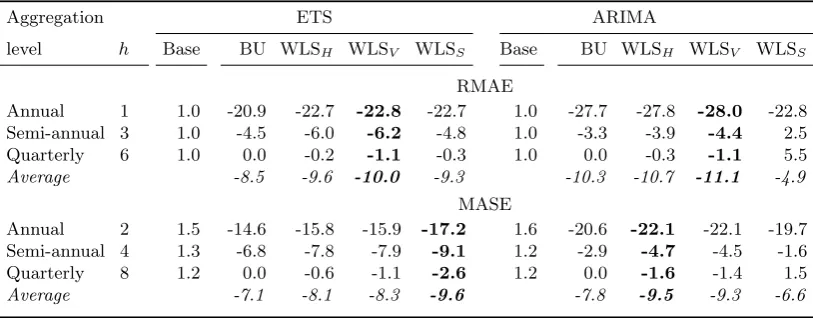
Aggregation ETS ARIMA

level h Base BU WLSH WLSV WLSS Base BU WLSH WLSV WLSS

RMAE

Annual 1 1.0 -20.9 -22.7 -22.8 -22.7 1.0 -27.7 -27.8 -28.0 -22.8 Semi-annual 3 1.0 -4.5 -6.0 -6.2 -4.8 1.0 -3.3 -3.9 -4.4 2.5 Quarterly 6 1.0 0.0 -0.2 -1.1 -0.3 1.0 0.0 -0.3 -1.1 5.5

Average -8.5 -9.6 -10.0 -9.3 -10.3 -10.7 -11.1 -4.9

MASE

Annual 2 1.5 -14.6 -15.8 -15.9 -17.2 1.6 -20.6 -22.1 -22.1 -19.7 Semi-annual 4 1.3 -6.8 -7.8 -7.9 -9.1 1.2 -2.9 -4.7 -4.5 -1.6 Quarterly 8 1.2 0.0 -0.6 -1.1 -2.6 1.2 0.0 -1.6 -1.4 1.5

Average -7.1 -8.1 -8.3 -9.6 -7.8 -9.5 -9.3 -6.6

Table 2: Results from forecasting the quarterly series. The entries in the column labelled ‘Base’ show the error measures for the base forecasts. The rest of the columns show the percentage differences between the reconciled forecasts and the base forecasts. A negative (positive) entry shows a decrease (increase) in the error measure. Reported figures are averages of the all forecasts up to and including the forecast horizonh.

between the ETS and ARIMA base forecasts; rather we aim to evaluate the performance of forecasting with temporal hierarchies using different base forecasts.

The monthly results presented in Table 1 clearly show that forecasting using temporal hierarchies results in significant forecast accuracy improvements for all aggregation levels over both ETS and ARIMA base forecasts, using either RMAE or MASE. The improvements are larger for ARIMA compared to ETS as the ARIMA base forecasts are less accurate than the ETS base forecasts and for both sets of forecasts they are largest at the annual level. Using

structural scaling, WLSS, generates the most accurate reconciled forecasts in this case. In

summary, the results show that combining forecasts from different aggregation levels results in more accurate forecasts than the independent base forecasts generated for each aggregation level separately. Hence, forecasting using temporal hierarchies results in forecasts that are not only reconciled, but also more accurate.

At the monthly level, the seasonal component of the time series dominates, potentially even masking the presence of any trend. At the higher aggregation levels, the seasonal dominance is attenuated while the low frequency components, such as the trend, become more prominent. This permits the models to capture this information more easily. At the annual level, estimation efficiency for the individual models generating the base forecasts is at its lowest due to the limited sample. The resulting forecasts from using temporal hierarchies bring the benefits of estimation efficiency and potential seasonal information from the lower levels to the annual level and take the trend information at the aggregate levels to the monthly level.

These effects are further highlighted by the performance of the BU forecasts. The BU forecasts show significant improvements over the base forecasts at the annual level. However at all levels below the annual there are very small improvements for the ARIMA forecasts and even losses for the ETS forecasts. This implies that at the intermediate levels, the independent base forecasts are more accurate than the BU forecasts. The BU forecasts, generated from the monthly data where estimation efficiency is at its maximum, are hindered by not using any additional views of the time series.

The quarterly results presented in Table 2 are similar to the monthly results, showing that the temporal hierarchy forecasts improve upon the base forecasts. In contrast to the monthly results, the quarterly BU forecasts are more accurate than the base forecasts. However forecasts from all three WLS estimators are more accurate than the BU forecasts for ETS, and forecasts

from WLSH and WLSV are more accurate than BU forecasts for ARIMA. The relative

im-provements in forecast accuracy in the BU forecasts from using quarterly data may signal that at this level some of the high frequency noise that was present at the monthly level is now filtered out and at the quarterly level we do not have the large efficiency losses we observe at the annual level. However, similar to the monthly results, the forecast improvements from using temporal hierarchies again show that it is beneficial to use the higher aggregation levels to improve estimates of the low frequency components of a time series while the higher frequency components are filtered out.

It is interesting to highlight some findings from both the monthly and quarterly data. Overall

temporal hierarchy forecasts, as encapsulated by WLSH, WLSV and WLSS, performed very

well, being more accurate than the base forecasts that would be produced if the time series were modelled in the conventional way. Despite the commonly accepted view that it is best to use BU with only the most disaggregated quarterly or monthly time series, our results show that combining information from all temporal aggregation levels is superior.

ETS and WLSS, while for the quarterly that was 9.70%, using ARIMA and WLSV. The other

scaling schemes provided similar results. Makridakis and Hibon (2000) report that the best result in the competition was achieved by the Theta method with 13.85% and 8.96% sMAPE for the monthly and quarterly series respectively.

The difference in the BU forecast accuracy between the monthly and the quarterly series is due to the quality of the lowest level forecasts. The monthly data did not allow us to accurately capture the trends often present in the time series of this dataset (this observation matches the findings by Kourentzes, Petropoulos and Trapero, 2014). This was not the case for the quarterly data. This suggests that temporal hierarchies will perform best when the base models are not necessarily capturing all the information in the most disaggregated time series. We investigate this in the next section as we evaluate the performance of these methods in a simulation setting.

6. A Monte-Carlo simulation study

The empirical experiment discussed in the previous section has shown that forecasting us-ing temporal hierarchies resulted in significant gains in forecastus-ing accuracy. We next design a simulation study in order to gain a greater understanding as to why these forecast improve-ments occur. We explore two simulation settings that enable us to provide further insights into forecasting using temporal hierarchies.

6.1. Simulation setting 1

In Silvestrini and Veredas (2008, Section 3.6), an ARIMA(0,0,1)(0,1,1)12 model with an

intercept is estimated for the Belgian public deficit series which comprises 252 monthly obser-vations. We use this estimated model at the monthly frequency (the estimated parameters of which are shown in the bottom row of Table 3) as our data generating process (DGP). Using the techniques surveyed in Silvestrini and Veredas (2008) we theoretically derive the parameters for the observationally equivalent representations of the monthly ARIMA DGP at each level of aggregation above the monthly level (see Table 3).

Aggregation

level ARIMA orders cˆ θˆ1 θˆ2 Θˆ1 σˆε

Derived models

Annual (0,1,2) 112.3 −0.43 0.01

Semi-annual (0,0,1)(0,1,1)2 28.1 −0.05 −0.4

Four-monthly (0,0,1)(0,1,1)3 12.4 −0.06 −0.4

Quarterly (0,0,1)(0,1,1)4 7.0 −0.10 −0.4

Bi-monthly (0,0,1)(0,1,1)6 3.1e−03 −0.13 −0.4

Estimated model

Monthly (0,0,1)(0,1,1)12 7.8e−04 −0.22 −0.4 4.19e−05

Table 3: Estimated parameters for the ARIMA DGP at the monthly frequency. Theoretically derived parameters for the observationally equivalent ARIMA representations for each aggregation level above the monthly level.

Drawing from normally distributed errors, εt∼N(0,σˆε2) where ˆσε2 is the estimate shown in

Table 3, we generate time series from the monthly DGP and then aggregate these to the levels above. Figure 4 shows a random draw from the simulations. For each time series generated at each aggregation level we generate four sets of base forecasts from:

Figure 4: Time series generated from the ARIMA DGP at the monthly frequency and aggregated at levelsk= {12,6,4,3,2,1}

Ann

ual

5 10 15 20

4.5

5.5

6.5

Quar

ter

ly

5 10 15 20

1.2

1.4

1.6

1.8

Semi−Ann

ual

5 10 15 20

2.4

2.8

3.2

3.6

Bi−Monthly

5 10 15 20

0.7

0.9

1.1

F

our−Monthly

5 10 15 20

1.6

2.0

2.4

Monthly

0 50 100 150 200 250

0.2

0.4

0.6

0.8

1. the theoretically derived ARIMA DGP;

2. the theoretically derived ARIMA DGP but with parameters estimated from the simulated data;

3. an automatically identified ARIMA model; 4. an automatically identified ETS model.

The automatically identified ARIMA and ETS models come from the forecast package for R as described in the preceding empirical section. Each set of base forecasts are reconciled applying the series variance scaling, proposed in Section 4, and using bottom-up forecasting. We do not report the figures for the hierarchy variance and structural scaling as the results were similar and did not change the rankings of the temporal hierarchy approach in the results that follow.

For each simulation setting, we generate samples at the monthly level of sizes n= 48,144, 240 and 480. For each sample size we consider forecast horizonsh∗ = 12,36,60,120 respectively. Equivalently, at the annual aggregation level, the samples sizes vary from 4 to 40 annual obser-vations with forecast horizons varying from 1 to 10 years ahead respectively. For each sample size we perform 1000 iterations. We have also experimented with other sample sizes, but to save space we only present these here.

Sample size: specified at the annual aggregation level

(Forecast horizon: specified at the annual aggregation level)

4 12 20 40 4 12 20 40 4 12 20 40 4 12 20 40

(1) (3) (5) (10) (1) (3) (5) (10) (1) (3) (5) (10) (1) (3) (5) (10)

Scenario 1 Scenario 2 Scenario 3 Scenario 4

WLS combination forecasts using variance scaling

Annual -0.3 0.0 0.0 0.0 -4.3 -7.9 -6.1 -3.3 -66.2 -5.1 -2.6 -0.4 -24.7 1.6 0.5 -1.8 Semi-annual -0.1 -0.1 0.0 0.0 -5.2 -3.5 -1.6 -0.2 -50.6 -4.9 -2.6 -1.2 -42.6 -5.5 -2.7 -1.1 Four-monthly -0.1 0.0 0.0 0.0 -3.8 -1.5 -0.4 -0.1 -10.1 -6.2 -2.0 -1.2 -9.4 -6.7 -2.7 -4.3 Quarterly -0.1 0.0 0.0 0.0 -3.9 -0.6 -0.2 -0.1 -16.4 -4.1 -1.9 -0.8 -1.2 -8.3 -5.5 -6.0 Bi-monthly 0.0 0.0 0.0 0.0 -1.1 0.0 0.1 0.0 -7.5 -3.3 -0.7 -0.9 -1.0 -8.3 -9.3 -8.6 Monthly 0.0 0.0 0.0 0.0 1.0 0.5 0.1 0.0 -0.9 -0.5 -0.8 -1.9 -1.4 -7.3 -11.3 -17.0

Bottom-up

Annual -0.7 -0.1 0.2 0.1 -5.3 -9.5 -7.1 -3.4 -64.2 -1.2 5.9 27.9 -20.9 69.1 101.6 150.4 Semi-annual -0.5 -0.1 0.1 0.0 -7.6 -4.8 -2.4 -0.2 -48.5 -2.8 2.3 13.8 -40.0 35.5 63.8 105.3 Four-monthly -0.2 -0.1 0.1 -0.1 -5.5 -2.7 -1.0 -0.2 -7.1 -5.1 1.4 8.7 -5.8 23.4 47.8 73.1 Quarterly -0.2 0.0 0.0 0.0 -6.1 -1.8 -0.7 -0.2 -14.0 -3.0 0.4 6.5 2.3 15.5 33.4 54.9 Bi-monthly -0.1 -0.1 0.0 0.0 -2.8 -0.9 -0.2 -0.1 -5.8 -2.4 1.2 3.8 1.9 8.2 16.1 32.7 Monthly 0.0 0.0 0.0 0.0 0.0 0.0 0.0 0.0 0.0 0.0 0.0 0.0 0.0 0.0 0.0 0.0

Table 4: Entries show the percentage differences in Root Mean Squared Error (RMSE) between base and rec-onciled forecasts. A negative (positive) entry represents a percentage decrease (increase) in RMSE relative to the base forecasts at that aggregation level. Scenario 1: base forecasts are generated from the theoretically derived ARIMA DGPs at each aggregation level; we have complete certainty at all levels. Scenario 2: base forecasts are generated from the theoretically derived ARIMA DGPs at each aggrega-tion level, however with estimated parameters; we have parameter estimaaggrega-tion uncertainty at each level. Scenario 3: base forecasts are generated from ARIMA models identified and estimated at each level from the data; we have model specification uncertainty. Scenario 4: base forecasts are generated from an ETS model; we are forecasting under model misspecification.

Scenario 1: Forecasting under complete certainty

The results for the first scenario are presented in the first panel of Table 4. Under this scenario all base forecasts are generated at all levels from the observationally equivalent DGPs and therefore we generate base forecasts under complete information at all levels. The percent-age differences between the WLS reconciled forecasts and the base forecasts are presented in the top half of the first panel. All percentage differences are zeros with the exception of some very small negative entries corresponding to minimal improvements in forecast accuracy over the base forecasts for sample sizes of 4 annual observations at the quarterly level and above. These small improvements in forecast accuracy result from the initial seed values playing a significant role in the generation of forecasts when the sample size is very small, as is the case for 4 observations at the annual level. For longer sample sizes the effect of the initial seed dies out.

This first simulation scenario acts as a control. From the results we are assured that the theoretical derivation of the observationally equivalent representations at each aggregation level has been correctly implemented. The conclusion from this scenario is that implementing the approach of temporal hierarchies when the base forecasts are accurate, which is the case here under complete certainty, does not cause any forecast accuracy loss. In fact it shows forecast improvements where some data generation and forecast generation discrepancies exist.

Scenario 2: forecasting under parameter uncertainty

Under this second scenario the base forecasts are generated from the theoretically derived observationally equivalent ARIMA DGPs at each level, however the parameters for each model are now estimated at each level. This scenario allows us to investigate the effect of parameter estimation efficiency loss on forecast accuracy.

The results are presented in the second panel of Table 4. All the entries for the bottom-up forecasts are negative. This is exactly expected. Using the bottom-up approach in this setting is the most efficient strategy. All bottom-up forecasts are derived from having estimated the correct model specification at the monthly level. The most efficient estimation of the correctly specified observationally equivalent DGPs is achieved at this very bottom aggregation level which provides estimation with the most degrees of freedom.

Compared to the bottom-up approach all the entries of the WLS reconciliation approach are smaller in magnitude and also all bottom level entries are positive (albeit very small). This is again exactly as expected. Under correct model specification combining forecasts from all levels to achieve reconciliation causes efficiency loss compared to the most efficient in this scenario bottom-up approach. However the gains in parameter estimation efficiency outweigh any losses from also using the base forecasts at the very bottom level in the combination approach. This makes the combination forecasts at all other levels more accurate than the base forecasts which we know are inefficient. As the sample size increases the differences between the BU and the WLS forecasts become smaller.

Scenario 3: forecasting under model specification uncertainty

Under this third scenario base forecasts are generated from automatically identified ARIMA models at each level. Therefore under this scenario we are studying the case where the fitted models are in the same class of models as the DGP, however the orders are possibly misspecified.

For small sample sizes the WLS reconciled forecasts show significant improvements in ac-curacy over the base forecasts especially at all levels above the monthly level. For example for the very small sample size of 4 annual observations, the WLS reconciled forecasts show a 66% improvement in RMSE over the base forecasts at the annual level. As we move down the aggregation levels these improvements decrease becoming small at the very bottom level. This shows that the individual models perform well in capturing and forecasting the dynamics at the monthly level but not so well in the levels above that and are particularly inaccurate at the annual level where there are only 4 observations. The temporal hierarchies approach using WLS reconciled forecasts, takes advantage of the accurate bottom level forecasts and combining these with forecasts from other levels improves the forecast accuracy for all the levels above. As the sample size increases, the individual models improve in capturing and projecting the strong trend resulting from the drift component of the ARIMA DGP, and therefore the improvements in the WLS reconciled forecasts diminish.

Scenario 4: forecasting under partial model misspecification

Under this fourth scenario, base forecasts are generated from an ETS model automatically identified at each level. There is no equivalent representation of the ARIMA(0,0,1)(0,1,1) DGP in the class of ETS models which is explored by the automatic algorithm. Therefore all base forecasts are generated by a misspecified model. The only exception is at the annual level, and this is reflected in the results. At the annual level the DGP is an ARIMA(0,1,2) and

the equivalent ETS representation is an ETS(A,Ad,N). For this level the ETS algorithm can

converge to the DGP and generate base forecasts from the observationally equivalent model. Hence for sample sizes larger than 4 annual observations, there are no significant improvements in forecasting accuracy from the WLS reconciled forecasts over the base forecasts at this level. However using the accurate base forecasts of the annual level in the WLS reconciled forecasts at the lower levels brings significant improvements over the base forecasts that have been generated from misspecified models.

The losses arising from using bottom-up forecasts from misspecified base models are sub-stantial. For samples larger than 4 annual observations, the increase in RMSE ranges from 69% to 150%. The misspecified base models at the bottom level are completely unable to capture the drift component of the ARIMA DGP at the levels above.

6.2. Simulation setting 2

In this second simulation setting we aim to generate time series with a much more erratically behaving trend in an attempt to limit the advantage of the base forecasts being relatively more accurate at the annual level compared to other levels. The DGP we generate from is an

ETS(A,Ad,A) model:

µt=ℓt−1+φbt−1+st−m

ℓt=ℓt−1+φbt−1+αεt

bt=φbt−1+βεt

st=st−m+γεt

ˆ

y_t+h|t=ℓt+φhbt+s_t−m+h+

m

whereφh =φ+· · ·+φh andh+m =

(h−1) modm

+ 1 (for more details see Hyndman et al., 2008). The parameters we generate from are ˆα= ˆβ = 0.0144,γˆ= 0.5521,φˆ= 0.9142. These are estimated from one random draw from the ARIMA DGP used in the first simulation setting. This DGP has one unit root and a second root near the unit circle as the dampening parameter is 0.91; consequently, the trend has somewhat erratic behaviour. Figure 5 plots two random draws from generating data from this DGP.

All results are presented in Table 5. Both sets of WLS reconciled forecasts show all around improvements over the base forecasts. The base forecasts generated by the ETS algorithm are most accurate now at the lower levels where more degrees of freedom can be utilized to get to the monthly DGP. Using these in the WLS combination assists the forecast accuracy of the WLS reconciled forecasts at the levels above. As expected, the ARIMA base forecasts are generally less accurate than the ETS forecasts and therefore the WLS reconciled forecasts show greater improvements over the base forecasts. The bottom-up forecasts now show better performance than the corresponding forecasts from scenarios 3 and 4 in simulation setup 1; however, in all cases they are clearly less accurate than the WLS reconciled forecasts which borrow information from all aggregation levels.

The simulations help us gain an insight as to when we should expect more improvements. Substantial improvements are possible with temporal hierarchies when our knowledge of the

Figure 5: Two random draws of time series generated from the ETS(A,Ad,A) DGP at the monthly frequency

and aggregated at levelsk={12,6,4,3,2,1}.

Ann

ual

5 10 15 20

2.6

2.8

3.0

Semi−Ann

ual

5 10 15 20

1.1 1.3 1.5 1.7 F our−Monthly

5 10 15 20

0.7 0.9 1.1 1.3 Quar ter ly

5 10 15 20

0.5

0.7

0.9

Bi−Monthly

5 10 15 20

0.2

0.4

0.6

Monthly

0 50 100 150 200 250

0.10 0.20 0.30 0.40 Ann ual

5 10 15 20

3.8 4.0 4.2 4.4 4.6 Semi−Ann ual

5 10 15 20

1.8 2.0 2.2 2.4 F our−Monthly

5 10 15 20

1.1 1.3 1.5 1.7 Quar ter ly

5 10 15 20

0.9

1.0

1.1

1.2

Bi−Monthly

5 10 15 20

0.4

0.6

0.8

Monthly

0 50 100 150 200 250

0.2

0.3

0.4

0.5

underlying DGP is very limited. This is also reflected in the results of the empirical evaluation, where on average we observed greater accuracy gains for the less accurate ARIMA base forecasts, relatively to ETS base forecasts. The temporal reconciliation regression model (5) suggests that

when the estimate of β(h) is close to the underlying true conditional mean of the observed

time series, then the reconciliation error will tend to zero. This happens when the bottom level forecasts originate from a model that matches the DGP, and is in accordance with our empirical and simulation observations.

Sample size: at the annual level

(Forecast horizon: at the annual level)

4 12 20 40 4 12 20 40

(1) (3) (5) (10) (1) (3) (5) (10)

ETS forecasts ARIMA forecasts

WLS combination forecasts using variance scaling

Annual -12.3 -5.4 -7.2 -9.8 -39.9 -7.6 -9.4 -1.0

Semi-annual -27.0 -3.6 -5.7 -4.2 -36.6 -1.4 -2.1 -0.8

Four-monthly -5.3 -3.6 -5.5 -1.6 -12.6 -4.1 -3.9 -2.6

Quarterly -2.3 -4.5 -5.1 -0.9 -23.9 -4.0 -4.4 -5.1

Bi-monthly -1.5 -4.0 -2.0 0.4 -11.6 -3.0 -3.6 -3.7

Monthly -1.5 -4.7 0.0 -2.0 -2.9 -2.6 -3.9 -5.1

Bottom-up

Annual -7.0 1.2 -6.7 -6.4 -36.4 -2.1 -2.6 5.9

Semi-annual 23.5 4.2 -5.3 -0.9 -33.6 3.8 4.4 6.2

Four-monthly -1.4 4.4 -5.1 1.6 -8.8 0.8 2.2 3.9

Quarterly 1.1 3.2 -4.8 2.1 -19.9 0.4 1.2 1.3

Bi-monthly 1.1 3.4 -1.9 3.0 -8.2 0.5 1.7 2.7

Monthly 0.0 0.0 0.0 0.0 0.0 0.0 0.0 0.0

Table 5: Entries show the percentage differences in RMSE between ETS and ARIMA base forecasts and recon-ciled forecasts. A negative (positive) entry represents a percentage decrease (increase) in RMSE relative to the base forecasts at that aggregation level.

bottom-up forecasts, while under increasing uncertainty, combining forecasts from the various levels of the hierarchy resulted in better forecasts over both benchmarks. We draw the conclu-sion that temporal hierarchies can be applied in all scenarios. Building on the good empirical performance and the simulation insights, we now use temporal hierarchies in a case study.

7. Case study: predicting accident and emergency service demand

To highlight the usefulness of temporal hierarchies for forecasting practice we consider the case of predicting the demand of Accident & Emergency (A&E) departments in the UK. Know-ing the future demand of A&E is needed for multiple plannKnow-ing decisions: for example man-agement needs to know the demand for the (a) short-term (1 month ahead) for staffing pur-poses; (b) medium-term (3 months ahead) for long-term staffing planning and procurement; and (c) long-term (1 year ahead) for staff training purposes. Very short-term forecasts (1 week or less ahead) may also be used to calibrate existing plans, for example arranging over-time sched-ules. Obviously, these plans need to be aligned to ensure the smooth operation and staffing of A&E departments (Izady and Worthington, 2012). Similar problems are faced by other hospi-tal operations, where “urgent” and “regular” patient demand must be satisfied (Truong, 2015), or more broadly in services where both scheduled and emergency jobs or repairs need to be conducted (Angalakudati et al., 2014).

A&E departments in the UK record a number of demand statistics, classified under three types: major A&E, single specialty and other/minor A&E. Each of these types requires dif-ferent resources and staffing. Furthermore, since 2004 a four-hour target was introduced for the emergency departments: at least 98% of patients should be seen, treated and subsequently admitted or discharged within four hours. This target was revised in 2010 to 95% of patients following concerns that the original target might be putting A&E departments under increased pressure, which might lead to compromising patient care (Mortimore and Cooper, 2007). In-sufficient numbers of inpatient beds, middle-grade doctors and nurses, and delays in accessing specialist opinions, have all been identified as key factors for not meeting the targets (Cooke et al., 2004; BMA, 2005). Therefore, it is felt that more accurate forecasts of the demand will allow for better planning and scheduling of resources, thus enabling A&E departments to meet their targets.

Weekly A&E demand data has been collected spanning 7 November 2010 to 7 June 2015. Table 6 lists the 13 demand series that were used in this case study, where total demand and demand satisfied within the 4 hours target were recorded. These reflect demand at a UK level.

Type 1 Departments — Major A&E Type 2 Departments — Single Specialty

Type 3 Departments — Other A&E/Minor Injury Unit Total Attendances

Type 1 Departments — Major A&E>4 hours

Type 2 Departments — Single Specialty>4 hours

Type 3 Departments — Other A&E/Minor Injury Unit>4 hours

Total Attendances >4 hours

Emergency Admissions via Type 1 A&E Total Emergency Admissions via A&E

Other Emergency Admissions (i.e not via A&E) Total Emergency Admissions

Number of patients spending>4 hours from decision to admit to admission

Table 6: The thirteen weekly A&E time series used in the case study.

Each time series is split into two subsets, a training set and an out-of-sample evaluation set. The latter spans the last 52 weeks of the time series, while all the remaining observations are used for fitting appropriate forecasting models. Each series is forecasted using ARIMA, which is specified as detailed in Section 5. Forecasts are first generated conventionally to give the base forecasts, and then temporal hierarchies are used with series variance scaling (WLSV).

The alternative scaling methods result in similar performance and therefore are not reported here. We use MASE to track the accuracy in predicting 1, 4 and 13 weeks ahead, matching the objectives described above. We use a rolling origin evaluation scheme, producing forecasts for all observations in the test set. This results in 40 different weekly forecasts up to 13 weeks ahead and a single one-step forecast at the annual level of aggregation. We report the average error across the different forecasts. The accuracy in predicting the total demand over the span of a complete year is tracked at the weekly and annual levels.

forecasts are also reconciled, supporting the alignment of the various decisions that need to be taken to run A&E departments.

Aggr. Level h Base Reconciled Change

Annual 1 3.4 1.9 −42.9%

Weekly 1–52 2.0 1.9 −5.0%

Weekly 13 2.3 1.9 −16.2%

Weekly 4 1.9 1.5 −18.6%

Weekly 1 1.6 1.3 −17.2%

Table 7: Average MASE for the base and temporally reconciled forecasts across all A&E time series, and per-centage change, for different forecast horizons (h). A negative entry indicates a percentage decrease in MASE for the reconciled forecasts compared to the base forecasts.

This becomes clearer by visualising the base and reconciled forecasts. As an example, Figure 6 plots the forecasts across the different aggregation levels for the Total Emergency Admissions time series.

The forecasts for the other series of the case study exhibit similar behaviour. The dashed line ( ) represents the base forecasts and the solid line ( ) the temporal hierarchy forecasts. To better illustrate the differences, predictions up to 2 years ahead are plotted. Focusing on the base forecasts, observe how different they are across the aggregation levels, which are associated with different planning levels and horizons. At the annual level there is no trend captured in the forecast, due to the limited fitting sample. The opposite is true for the other levels, while for the weekly level the captured trend seems very weak and improbable given the historical demand. Similarly seasonality is captured relatively accurately in the quarterly, monthly and bi-weekly levels, but not at the weekly level. Comparing the forecasted A&E admissions over the duration of a complete year at the weekly and the annual levels, we can observe that the forecasts result in a different average level of demand. Therefore, apart from the low accuracy of the base forecasts as is evident from Table 7, there is substantial disagreement between levels and in turn between short and long planning horizons. This can lead to conflicting decisions, for example between the long-term plans for staff training and the short to mid-term plans for staffing levels and scheduling.

On the other hand, the reconciled forecasts combine information contained in the different aggregation levels. The trend identified at the lower levels contributes to the forecasts at the annual level, resulting in more accurate predictions. This is also reflected in the projected sea-sonality at the weekly level. Overall, we infer that by using temporal hierarchies the modelling uncertainty at each individual level is reduced. The forecasts produced across the various levels, capturing different parts of the information contained within the time series, are combined into an accurate and robust forecast, which can be aggregated or disaggregated as needed. This results in reconciled predictions. Plans at any level and horizon are now based on identical forecasts and therefore will be aligned. The operational scheduling of available staff and the tactical decision on staffing levels can be aligned. Similarly, patient bed capacity can be planned accordingly while ensuring adequate number of nurses and doctors to make use of them; and (at a longer horizon) to train them accordingly. The reconciliation of the forecasts across forecast horizons and levels enables consistency across the various decisions required to meet the A&E service targets and smooth operations.

In this case study we have demonstrated that the application of temporal hierarchies can be beneficial for the activities of A&E departments. The main gain is decision making alignment, while a beneficial by-product is significantly improved accuracy.

Figure 6: Predictions for the Total Emergency Admissions time series (in 000s). Forecasts are plotted in the greyed area. Dashed line ( ) is used for the base forecasts and solid line ( ) for the temporal hierarchy forecasts.

1 2 3 4 5 6

5100

5300

5500

Annual (k=52)

Forecast

2 4 6 8 10 12

2500

2600

2700

2800

2900

Semi−annual (k=26)

Forecast

5 10 15 20 25

1250

1350

1450

Quarterly (k=13)

Forecast

20 40 60 80

360

380

400

420

440

460

Monthly (k=4)

Forecast

50 100 150

180

190

200

210

220

230

Bi−weekly (k=2)

Forecast

50 100 150 200 250 300

90

95

100

105

110

Weekly (k=1)

Forecast

8. Conclusions

This paper introducesTemporal Hierarchies, a novel approach for modelling and forecasting time series. Forecasting with temporal hierarchies involves using non-overlapping aggregation to temporally aggregate time series up to the annual level, generating forecasts for each ag-gregate series independently, and then optimally combining these to produce forecasts that are reconciled across short, medium and long-term forecast horizons. Our results are threefold: an extensive empirical evaluation, forecasting the 2,184 monthly and quarterly series of the M3 competition; a comprehensive simulation study providing useful insights of the approach; and a detailed case study using weekly data to forecast demand of A&E departments in the UK across different planning horizons. Besides generating forecasts that are reconciled across differ-ent forecast horizons (which is important in order to align managerial decision making), all our results uniformly point towards one conclusion: forecasting with temporal hierarchies results to significant forecast accuracy improvements across all forecast horizons.

Obviously the next step is an integrated hierarchical forecast that will result in consistent forecasts for organisations to base their plans and decisions on. Temporal hierarchies align the planning horizons, while cross-sectional hierarchies align for a single time unit the forecasts across different items. These two concepts can be combined into cross-temporal hierarchical forecasts that will be reconciled across all dimensions resulting in a ‘one-number forecast’, thus providing decision making transparency to organisations across products, segments, markets, etc. and decision horizons; leading to harmonised actions.

References

Abraham, B. (1982), ‘Temporal Aggregation and Time Series’,International Statistical Review / Revue Interna-tionale de Statistique50(3), 285–291.

Amemiya, T. and Wu, R. Y. (1972), ‘The Effect of Aggregation on Prediction in the Autoregressive model’,

Journal of the American Statistical Association67(339), 628–632.

Andrawis, R. R., Atiya, A. F. and El-Shishiny, H. (2011), ‘Combination of long term and short term forecasts, with application to tourism demand forecasting’,International Journal of Forecasting27(3), 870–886. Angalakudati, M., Balwani, S., Calzada, J., Chatterjee, B., Perakis, G., Raad, N. and Uichanco, J. (2014),

‘Ran-dom Emergencies Business Analytics for Flexible Resource Allocation Under Ran‘Ran-dom Emergencies’, Manage-ment Science60(6), 1552–1573.

Ashton, a. H. and Ashton, R. H. (1985), ‘Aggregating Subjective Forecasts: Some Empirical Results’, Manage-ment Science31(12), 1499–1508.

Athanasopoulos, G., Ahmed, R. A. and Hyndman, R. J. (2009), ‘Hierarchical forecasts for Australian domestic tourism’,International Journal of Forecasting25, 146–166.

Bates, J. M. and Granger, C. W. J. (1969), ‘The combination of forecasts’, Operational Research Quarterly

20(4), 451–468.

BMA (2005), BMA survey of A&E waiting times, Technical report, British Medical Association.

Breiman, L. et al. (1996), ‘Heuristics of instability and stabilization in model selection’,The annals of statistics

24(6), 2350–2383.

Brewer, K. (1973), ‘Some consequences of temporal aggregation and systematic sampling for ARMA and ARMAX models’,Journal of Econometrics1(2), 133–154.

Budescu, D. V. and Chen, E. (2014), ‘Identifying Expertise to Extract the Wisdom of Crowds’, Management Science61(2), 267–280.

Clemen, R. T. (1989), ‘Combing forecasts - a review and annotated-bibliography’, International Journal of Forecasting5(4), 559–583.

Cooke, M., Wilson, S., Halsall, J. and Roalfe, A. (2004), ‘Total time in english accident and emergency depart-ments is related to bed occupancy’,Emergency Medicine Journal21(5), 575–576.

Davydenko, A. and Fildes, R. (2013), ‘Measuring Forecasting Accuracy: The Case Of Judgmental Adjustments To Sku-Level Demand Forecasts’,International Journal of Forecasting29(3), 510–522.

Elliott, G. and Timmermann, A. (2004), ‘Optimal forecast combinations under general loss functions and forecast error distributions’,Journal of Econometrics122(1), 47–79.

Elliott, G. and Timmermann, A. (2005), ‘Optimal forecast combination under regime switching’,International Economic Review46(4), 1081–1102.

Fliedner, G. (2001), ‘Hierarchical forecasting: issues and use guidelines’,Industrial Management & Data Systems

101(1), 5–12.

Goodwin, P. (2000), ‘Correct or combine? Mechanically integrating judgmental forecasts with statistical meth-ods’,International Journal of Forecasting16(2), 261–275.

Gross, C. W. and Sohl, J. E. (1990), ‘Disaggregation methods to expedite product line forecasting’,Journal of Forecasting9, 233–254.

Hotta, L. K. (1993), ‘The effect of additive outliers on the estimates from aggregated and disaggregated ARIMA models’,International Journal of Forecasting9(1), 85–93.

Hotta, L. K. and Cardoso Neto, J. (1993), ‘The effect of aggregation on prediction in autoregressive integrated moving-average models’,Journal of Time Series Analysis14(3), 261–269.

Hyndman, R. J. (2015),forecast: Forecasting functions for time series and linear models. R package version 6.1.

URL:cran.r-project.org/package=forecast

Hyndman, R. J., Ahmed, R. A., Athanasopoulos, G. and Shang, H. L. (2011), ‘Optimal combination forecasts for hierarchical time series’,Computational Statistics & Data Analysis55(9), 2579–2589.

Hyndman, R. J. and Khandakar, Y. (2008), ‘Automatic time series forecasting: The forecast package forR_’, Journal of Statistical Software27(3), 1–22.

Hyndman, R. J. and Koehler, A. B. (2006), ‘Another look at measures of forecast accuracy’,International Journal of Forecasting22, 679–688.