Returns to tail hedging

Returns to tail hedging

Bell, Peter N

University of Victoria

13 February 2015

Online at

https://mpra.ub.uni-muenchen.de/62160/

Running head: TAIL HEDGING 1

© Peter Bell, 2015

Returns to tail hedging

Peter N. Bell

Department of Economics, University of Victoria

Author note

Contact information: [email protected], 250 588 6939.

Abstract

Tail hedging is a portfolio management strategy meant to reduce the risk of large losses. For an

investor who holds a stock market index fund, the strategy entails buying out of the money put

options on the index. Research suggests the strategy works well in practice and I explore the

returns to tail hedging in a simple theoretical model. I calculate descriptive statistics for the

returns to tail hedging when the stock price has either a normal or fat tailed distribution. I find

that tail hedging is rewarding when stock prices have fat tails.

Keywords: Portfolio management, tail option, fat tail, simulation.

TAIL HEDGING 3

Returns to tail hedging

1. Introduction

Diversification can reduce risk in a stock portfolio, but cannot eliminate the risk of large

losses due to widespread crisis. Investors can reduce this risk by using a technique called tail

hedging, which entails buying out of the money put options. However, tail hedging requires

specific expertise to trade in illiquid options and portfolio managers’ time may be better spent

assessing their investments than preparing for systemic crises. This creates an opportunity for

firms like Universa Investments to provide tail hedging services to institutional investors.

Spitznagel, Yarckin, Mann (2015), who are affiliated with Universa Investments, describe the

performance of a typical tail hedging strategy from 2004-2014. They find that the strategy has

higher risk adjusted returns than many other types of portfolios. The evidence suggests that tail

hedging works in practice, but does it work in theory?

Spitznagel, Yarckin, Mann (2015) describe a simple tail hedged portfolio as one unit of the

SP500 index and several out of the money put options on the index. They roll the options

positions as they expire in order to ensure that “the tail-hedged portfolio breaks even for a down

20% move in the S&P 500 over a month” (2015, p.2). It is possible to construct such a portfolio

of options in different ways based on the expiry dates, strike prices, and quantity of options used.

However, the authors state simply that they buy “one delta which has a strike roughly 30-35%

below spot” (2015, p.2), which helps me determine ballpark figures for appropriate quantity of

options and strike price for a tail hedged portfolio.

I use a simple model with two time periods to explore tail hedging in theory. At the initial

expires and they calculate their returns. I use simulation to estimate the distribution of returns

under different assumptions about the data generating process and investor portfolio. I consider

an unhedged portfolio in stock, a fully hedged portfolio where the notional value of the put

option equals the value of the stock, an over-hedged portfolio where the notional is larger, and a

portfolio where the investor only buys put options. For each portfolio, I simulate stock returns

according to either a normal or fat tail distribution. However, I always use the Black-Scholes

option price to create some mispricing in options that could make tail hedging particularly

valuable.

2. Model

I denote stock price at expiry as Si where the returns are either normal i=Z or fat tailed i=T.

The normal model is given in Equation (1), where Zis a standard normal random variable. The

average return is µ=0 and standard deviation is σ=0.10. The initial stock price is S0=100.

( 1 ) SZ= S0e x p (µ+σZ) .

The fat tail model for stock prices is given in Equation (2). I assume returns have a T(v)

distribution, with degree of freedom v>2. I use v=8 to create a mild degree of fat tails in the

returns. As before, the average return is µ=0 and initial price S0=100. However, to ensure that

the standard deviation of returns under fat tails is equal to the normal model, I use a different

scale parameter σT. I use σT=σ/s(T) where s() denotes sample estimate of standard deviation for

the T variable.

( 2 ) ST= S0exp(µ+σTT ) .

Throughout the paper, I calculate the put option price P using Black-Scholes model as in

TAIL HEDGING 5

which implies that the options are mispriced when stock returns have fat tails. I assume the

option price uses true volatility, σ=0.10, time to expiry is τ=1, and the interest rate is zero r=0.

( 3 ) d1=(1/σ√τ)( l o g ( S0/ K ) + ( r + ½σ2)τ) , d2= d1-σ√τ.

( 4 ) P = K e-r τΦ(- d2)–S0Φ(- d1) .

I calculate the agent’s wealth at expiry as in Equation (5). I denote the quantity of put

options in the portfolio as qP and quantity of stock as qS.

( 5 ) W ( Si) = qSSi+ qP( m a x [ K - Si, 0 ] ) .

I calculate the distribution for wealth at expiry and returns as in Equation (6). I denote returns

as R(qS,qP,K) to emphasize the key variables: quantity of options qp, stock qS, and strike price K.

I consider different combinations of values for these variables to explore different types of

portfolios.

( 6 ) R ( qS, qP, K ) = W ( Si) / ( qSS0+ qPP )

To analyze the model, I specify all parameters above and draw a sample of observations on

the stock price with sample size n=107. I use the sample to estimate the distribution of returns

for the portfolio, then discuss several statistics that characterize the distribution.

3. Results

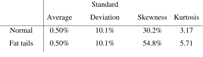
The first portfolio that I consider is an unhedged portfolio, with qS=1, qP=0. I report statistics

from the distribution of returns under both the normal and fat tail model in Table 1. The table

shows that the average and standard deviation of returns are equal for the normal and fat tail

models, but the skewness and kurtosis is larger in the fat tail model. These two features occur by

Table 1: Statistics for returns with unhedged portfolio

Average

Standard

Deviation Skewness Kurtosis

Normal 0.50% 10.1% 30.2% 3.17

Fat tails 0.50% 10.1% 54.8% 5.71

Table 2 describes returns with a tail hedge, qS=1, qP=1, and K=0.8S0. The statistics suggest

that the tail hedge has a very small effect on the distribution of returns, but the effect is apparent.

Notice how the skewness increases and kurtosis decreases for both the normal and fat tail model,

this occurs because the tail option removes extreme downward move in portfolio. Notice also

how the average returns increase and standard deviation of returns decrease under the fat tail

model. In other words, the tail hedge improves the risk adjusted returns under the fat tail model.

This encouraging result suggests it may be valuable to consider a larger tail hedge where qP>1.

Table 2: Statistics for returns with tail hedge

Average

Standard

Deviation Skewness Kurtosis

Normal 0.50% 9.99% 35.4% 3.09

Fat tails 0.53% 9.94% 69.8% 5.61

Table 3 describes returns with an extremely large tail hedge, qS=1, qP=10, and K=0.8S0. The

results show that a large tail hedge decreases average returns under the normal model, but

actually increases them under fat tails. Although the standard deviation of returns increase in

this case, the average returns increase even faster, which suggests that a large tail hedge can

improve risk adjusted returns even further. However, these gains may be due to the fact that the

TAIL HEDGING 7

Table 3: Statistics for returns with large tail hedge

Average Standard Deviation Skewness Kurtosis

Normal 0.45% 9.99% 62% 4.63

Fat tails 0.82% 11.1% 311% 41.72

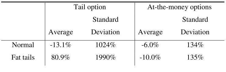
Table 4 describes returns when an investor buys put options with no stock, qS=0 and qP=1.

One section of the results describes returns with a tail option K=0.8S0 and the other describes an

option with strike at-the-money K=S0. The average returns are generally negative because

options function as insurance. However, the results show that buying tail options under the fat

tail model provides large positive average returns relative to the cost of option (80.9%). This

large return is due to the mispricing of options under fat tails, which is related to the trading

activities of Spitznagel and Nassim Taleb at Empirica Capital.

Table 4: Statistics for returns with buying naked put options

Tail option At-the-money options

Average

Standard

Deviation Average

Standard

Deviation

Normal -13.1% 1024% -6.0% 134%

Fat tails 80.9% 1990% -10.0% 135%

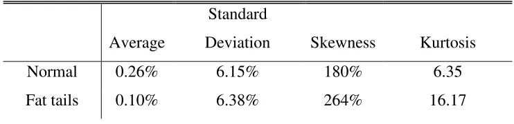
Table 5 describes returns with an at-the-money hedge, qS=1, qP=1, K=S0. The average

returns are much lower than the unhedged portfolio for both models because at-the-money

options are much more expensive than tail options. However, the options also cause the standard

deviation of returns to decrease substantially. These results begin to show just how different it

Table 5: Statistics for returns with at-the-money hedge

Average

Standard

Deviation Skewness Kurtosis

Normal 0.26% 6.15% 180% 6.35

Fat tails 0.10% 6.38% 264% 16.17

Although the differences between the average returns in this section are generally very small,

keep in mind that 1/100th of one percent is known as a basis points in finance and serves a useful

function for measuring returns. Furthermore, it is not clear from my analysis that the differences

described here are statistically significant. However, I would suggest that the differences are

economically significant because I am working with a model of one time step. In practice, these

differences can be compounded over many periods and grow to a large amount.

4. Discussion

I present a simple theoretical model to explore the distribution of returns for portfolios with

tail hedging. I compare portfolio returns when prices are generated according to a normal

probability model versus one with fat tails and show that tail hedging is associated with an

increase in risk adjusted returns under the fat tail model, which may be driven by the fact that the

options are underpriced in this model.

It is possible to extend the analysis presented here in several ways. One way is to use

another measure of risk to compare portfolios. Spitznagel, Yarckin, Mann (2015) use

semi-variance instead of semi-variance because it only measures downward variation in prices and the

benefits of tail hedging may be even more apparent using that measure than standard deviation.

TAIL HEDGING 9

theoretical model with more time steps would allow for a more sophisticated tail hedging

strategy, such as scaling in or out of options positions over time, and important stylized features

of financial time series, such as volatility clustering. I believe there are many opportunities to

develop theory to better understand the empirical results described by Spitznagel, Yarckin, Mann

References

Spitznagel, M., Yarckin, B., Mann, C. (2015, January). Capital asset pricing mistakes.