ConnotationWordNet: Learning Connotation over the Word+Sense Network

ConnotationWordNet:

Learning Connotation over the Word+Sense Network

Department of Computer Science Stony Brook University Stony Brook, NY 11794-4400

junkang, songfeng, leman, [email protected]

Abstract

We introduceConnotationWordNet, a con-notation lexicon over the network ofwords

in conjunction withsenses. We formulate the lexicon induction problem as collec-tive inference over pairwise-Markov Ran-dom Fields, and present a loopy belief propagation algorithm for inference. The key aspect of our method is that it is thefirst unified approach that assigns the polarity of both word- and sense-level connotations, exploiting the innate bipar-tite graph structure encoded in WordNet. We present comprehensive evaluation to demonstrate the quality and utility of the resulting lexicon in comparison to existing connotation and sentiment lexicons. 1 Introduction

We introduceConnotationWordNet, a connotation lexicon over the network ofwordsin conjunction withsenses, as defined in WordNet. A connotation lexicon, as introduced first by Feng et al. (2011), aims to encompass subtle shades of sentiment a word may conjure, even for seemingly objective words such as “sculpture”, “Ph.D.”, “rosettes”. Understanding the rich and complex layers of con-notation remains to be a challenging task. As a starting point, we study a more feasible task of learning thepolarityof connotation.

For non-polysemous words, which constitute a significant portion of English vocabulary, learning the general connotation at the word-level (rather than at the sense-level) would be a natural oper-ational choice. However, for polysemous words, which correspond to most frequently used words, it would be an overly crude assumption that the same connotative polarity should be assigned for all senses of a given word. For example, consider

“abound”, for which lexicographers of WordNet

prescribe two different senses:

• (v)abound: (be abundant of plentiful; exist in large quantities)

• (v)abound, burst, bristle: (be in a state of movement or action) “The room abounded with screaming children”;“The garden bris-tled with toddlers”

For the first sense, which is the most commonly used sense for“abound”, the general overtone of the connotation would seem positive. That is, al-though one can use this sense in both positive and negative contexts, this sense of“abound” seems to collocate more often with items that are good to be abundant (e.g.,“resources”), than unfortunate items being abundant (e.g.,“complaints”).

However, as for the second sense, for which

“burst”and“bristle”can be used interchangeably with respect to this particular sense,1 _{the general}

overtone is slightly more negative with a touch of unpleasantness, or at least not as positive as that of the first sense. Especially if we look up the Word-Net entry for“bristle”, there are noticeably more negatively connotative words involved in its gloss and examples.

This word sense issue has been a universal chal-lenge for a range of Natural Language Processing applications, including sentiment analysis. Recent studies have shown that it is fruitful to tease out subjectivity and objectivity corresponding to dif-ferent senses of the same word, in order to improve computational approaches to sentiment analysis (e.g. Pestian et al. (2012), Mihalcea et al. (2012) Balahur et al. (2014)). Encouraged by these recent successes, in this study, we investigate if we can attain similar gains if we model the connotative polarity of senses separately.

There is one potential practical issue we would like to point out in building a sense-level lexical resource, however. End-users of such a lexicon may not wish to deal with Word Sense Disam-1_{Hence asensein WordNet is defined bysynset (=} syn-onym set), which is the set of words sharing the same sense.

biguation (WSD), which is known to be often too noisy to be incorporated into the pipeline with re-spect to other NLP tasks. As a result, researchers often would need to aggregate labels across differ-ent senses to derive the word-level label. Although such aggregation is not entirely unreasonable, it does not seem to be the most optimal and princi-pled way of integrating available resources.

Therefore, in this work, we present the first uni-fied approach that learns both sense- and word-level connotations simultaneously. This way, end-users will have access to more accurate sense-level connotation labels if needed, while also having ac-cess to more general word-level connotation la-bels. We formulate the lexicon induction problem as collective inference over pairwise-Markov Ran-dom Fields (pairwise-MRF) and derive a loopy be-lief propagation algorithm for inference.

The key aspect of our approach is that we ex-ploit the innate bipartite graph structure between words and senses encoded in WordNet. Although our approach seems conceptually natural, previous approaches, to our best knowledge, have not di-rectly exploited these relations between words and senses for the purpose of deriving lexical knowl-edge over words and senses collectively. In ad-dition, previous studies (for both sentiment and connotation lexicons) aimed to produce only ei-ther of the two aspects of the polarity: word-level or sense-level, while we address both.

Another contribution of our work is the intro-duction of loopy belief propagation (loopy-BP) as a lexicon induction algorithm. Loopy-BP in our study achieves statistically significantly better performance over the constraint optimization ap-proaches previously explored. In addition, it runs much faster and it is considerably easier to imple-ment. Last but not least, by using probabilistic rep-resentation of pairwise-MRF in conjunction with Loopy-BP as inference, the resulting solution has the natural interpretation as the intensity of con-notation. This contrasts to approaches that seek discrete solutions such as Integer Linear Program-ming(Papadimitriou and Steiglitz, 1998).

ConnotationWordNet, the final outcome of our study, is a new lexical resource that has conno-tation labels over both words and senses follow-ing the structure of WordNet. The lexicon is pub-licly available at: http://www.cs.sunysb.

edu/˜junkang/connotation_wordnet.)

In what follows, we will first describe the

net-memberships)

antonyms)

Pred1Arg)

Arg1Arg)

…)

…)

prevent)

suffer)

enjoy)

achieve)

pain)

losses)

life)

profit)

success) win)

investment) injure) accident)

wound) ache)

word) sense)

gain) hurt)

put)on) lose)

injure,)) wound)

gain,)) put)on) win,)gain,) acquire) win,)profits,))) winnings)

ConnotaAve)

Predicates) Arguments) Senses)

Figure 1: GWORD+SENSE_{with words and senses.}

work of words and senses (Section 2), then intro-duce the representation of the network structure as pairwise Markov Random Fields, and a loopy be-lief propagation algorithm as collective inference (Section 3). We then present comprehensive eval-uation (Section 4 & 5 & 6), followed by related work (Section 7) and conclusion (Section 8). 2 Network of Words and Senses

The connotation graph, called GWORD+SENSE_{, is a}

heterogeneous graph with multiple types of nodes and edges. As shown in Figure 1, it contains two types of nodes; (i) lemmas (i.e., words, 115K) and (ii) synsets (63K), and four types of edges; (t1) predicate-argument (179K), (t2) argument-argument (144K), (t3) argument-synset (126K), and (t4) synset-synset (3.4K) edges.

The predicate-argument edges, first introduced by Feng et al. (2011), depict the selectional prefer-ence of connotative predicates (i.e., the polarity of a predicate indicates the polarity of its arguments) and encode their co-occurrence relations based on the Google Web 1T corpus. The argument-argument edges are based on the distributional similarities among the arguments. The argument-synset edges capture the synonymy between argu-ment nodes through the corresponding synsets. Fi-nally, the synset-synset edges depict the antonym relations between synset pairs.

receive the same connotation label. Conversely, we expect that these edges will also encourage

words that belong to the same sense (i.e., synset definition) to receive the same connotation label.

Another benefit of our approach is that for var-ious WordNet relations (e.g., antonym relations), which are defined over synsets (not over words), we can add edges directly between corresponding synsets, rather than projecting (i.e., approximat-ing) those relations over words. Note that the lat-ter, which has been employed by several previous studies (e.g., Kamps et al. (2004), Takamura et al. (2005), Andreevskaia and Bergler (2006), Su and Markert (2009), Lu et al. (2011), Kaji and Kit-suregawa (2007), Feng et al. (2013)), could be a source of noise, as one needs to assume that the semantic relation between a pair of synsets trans-fers over the pair of words corresponding to that pair of synsets. For polysemous words, this as-sumption may be overly strong.

3 Pairwise Markov Random Fields and Loopy Belief Propagation

We formulate the task of learning sense- and word-level connotation lexicon as a graph-based clas-sification task (Sen et al., 2008). More formally, we denote the connotation graph GWORD+SENSE_by

G= (V, E), in which a total ofnword and synset nodes V = {v1, . . . , vn} are connected with

typed edges e(vi, vj, t) ∈ E, where edge types t ∈ {pred-arg, arg-arg, syn-arg, syn-syn} de-pict the four edge types as described in Section 2. A neighborhood function N, where Nv =

{u|e(u, v) ∈ E} ⊆ V, describes the underlying network structure.

In our collective classification formulation, each node inV is represented as a random variable that takes a value from an appropriate class label do-main; in our case, L = {+,−} for positive and negative connotation. In this classification task, we denote byYthe nodes the labels of which need to be assigned, and letyirefer toYi’s label.

3.1 Pairwise Markov Random Fields

We next define our objective function. We pro-pose to use an objective formulation that utilizes pairwise Markov Random Fields (MRFs) (Kinder-mann and Snell, 1980), which we adapt to our problem setting. MRFs are a class of probabilistic graphical models that are suited for solving infer-ence problems in networked data. An MRF

con-sists of an undirected graph where each node can be in any of a finite number of states (i.e., class labels). The state of a node is assumed to be de-pendent on each of its neighbors and indede-pendent of other nodes in the graph.2 _{In pairwise MRFs,}

the joint probability of the graph can be written as a product of pairwise factors, parameterized over the edges. These factors are referred to as clique potentials in general MRFs, which are essentially functions that collectively determine the graph’s joint probability.

Specifically, let G = (V, E)denote a network of random variables, whereV consists of the un-observed variablesYthat need to be assigned val-ues from label setL. LetΨdenote a set of clique potentials that consists of two types of factors:

• For eachYi ∈ Y, ψi ∈ Ψ is a prior map-pingψi :L →R≥0, whereR≥0denotes non-negative real numbers.

• For eache(Yi, Yj, t)∈E,ψt

ij ∈Ψis a com-patibilitymappingψt

ij :L × L →R≥0.

Objective formulation Given an assignmenty

to all the unobserved variables Y and x to ob-served ones X (variables with known labels, if any), our objective function is associated with the following joint probability distribution

P(y|x) = _Z(1_x) Y Yi∈Y

ψi(yi) Y

e(Yi,Yj,t)∈E

ψt_ij(yi, yj)

(1) whereZ(x)is the normalization function. Our goal is then to infer the maximum likelihood as-signment of states (i.e., labels) to unobserved vari-ables (i.e., nodes) that will maximize Equation (1).

Problem Definition Having introduced our graph-based classification task and objective for-mulation, we define our problem more formally.

Given

- a connotation graph G = (V, E) of words and synsets connected withtypededges, - priorknowledge (i.e., probabilities) of (some

or all) nodes belonging to each class,

- compatibilityof two nodes with a given pair of labels being connected to each other;

Classifythe nodesYi∈ Y, into one of two classes; L = {+,−}, such that the class assignments yi

maximize our objective in Equation (1).

We can furtherrankthe network objects by the probability of their connotation polarity.

3.2 Loopy Belief Propagation

Finding the best assignments to unobserved vari-ables in our objective function is the inference problem. The brute force approach through enu-meration of all possible assignments is exponen-tial and thus intractable. In general, exact in-ference is known to be NP-hard and there is no known algorithm which can be theoretically shown to solve the inference problem for gen-eral MRFs. Therefore in this work, we em-ploy a computationally tractable (in fact linearly scalable with network size) approximate infer-ence algorithm called Loopy Belief Propagation (LBP) (Yedidia et al., 2003), which we extend to handle typed graphs like our connotation graph.

Our inference algorithm is based on iterative message passing and the core of it can be concisely expressed as the following two equations:

mi→j(yj) =α X

yi∈L

ψt

ij(yi, yj)ψi(yi)

Y

Yk∈Ni∩Y\Yj

mk→i(yi)

, ∀yj ∈ L (2)

bi(yi) =β ψi(yi) Y

Yj∈Ni∩Y

mj→i(yi),∀yi ∈ L

(3) A messagemi→j is sent from nodeito nodej

and captures the belief of iaboutj, which is the probability distribution over the labels of j; i.e. whati “thinks”j’s label is, given the current la-bel ofi and the type of the edge that connects i

and j. Beliefs refer to marginal probability dis-tributions of nodes over labels; for examplebi(yi)

denotes thebeliefof nodeihaving labelyi.αand β are the normalization constants, which respec-tively ensure that each message and each set of marginal probabilities sum to1. At every iteration, each node computes its belief based on messages received from its neighbors, and uses the compat-ibility mapping to transform its belief into mes-sages for its neighbors. The key idea is that after enough iterations of message passes between the nodes, the “conversations” are likely to come to a consensus, which determines the marginal proba-bilities of all the unknown variables.

The pseudo-code of our method is given in Al-gorithm 1. It first initializes all messages to 1

and priors to unbiased (i.e., equal) probabilities for all nodes except the seed nodes for which the sentiment is known (lines 3-9). It then proceeds by making each Yi ∈ Y communicate messages

Algorithm 1:CONNOTATIONINFERENCE

1 Input:Connotation graphG=(V, E), prior

potentialsψsfor seed wordss∈S, and compatibility potentialsψt

ij

2 Output: Connotation label probabilities for

each nodei∈V\P

3 foreache(Yi, Yj, t)∈Edo//initialize msg.s 4 foreachyj ∈ Ldo

5 m_i→j(y_j)←1

6 foreachi∈V do//initialize priors 7 foreachy_j ∈ Ldo

8 ifi∈Sthenφi(yj)←ψi(yj)else

φi(yj)←1/|L|

9 repeat //iterative message passing

10 foreache(Y_i, Y_j, t)∈E,Y_j ∈ YV\Sdo

11 foreachyj ∈ Ldo

12 Use Equation (2)

13 untilall messages stop changing

14 foreachYi∈ YV\Sdo//compute final beliefs 15 foreachy_i∈ Ldo

16 Use Equation (3)

with their neighbors in an iterative fashion until the messages stabilize (lines 10-14), i.e. conver-gence is reached.3 _{At convergence, we calculate}

the marginal probabilities, that is of assigning Yi

with labelyi, by computing the final beliefsbi(yi)

(lines 15-17). We use these maximum likelihood probabilities for label assignment; for each nodei, we assign the labelLi ←maxyibi(yi).

To completely define our algorithm, we need to instantiate the potentialsΨ, in particular the priors and the compatibilities, which we discuss next.

Priors Thepriorbeliefsψiof nodes can be suit-ably initialized if there is any prior knowledge for their connotation sentiment (e.g.,enjoy is posi-tive, sufferis negative). As such, our method is flexible to integrate available side information. In case there is no prior knowledge available, each node is initialized equally likely to have any of the possible labels, i.e., 1

|L| as in Algorithm 1 (line 9).

Compatibilities The compatibility potentials can be thought of as matrices, with entries

3_{Although convergence is not theoretically guaranteed, in} practice LBP converges to beliefs within a small threshold of change (e.g.,10−6_{) fairly quickly with accurate results}

ψt

ij(yi, yj)that give the likelihood of a node

hav-ing labelyi, given that it has a neighbor with label yj to which it is connected through a typetedge. A key difference of our method from earlier mod-els is that we use clique potentials that differ for edge types, since the connotation graph is hetero-geneous. This is exactly because the compatibil-ity of class labels of two adjacent nodes depends on the type of the edge connecting them: e.g.,

+ −−−−−→syn-arg + is highly compatible, whereas + syn-syn

−−−−−→+is unlikely; assyn-arg edges capture synonymy; i.e., words-sense memberships, while

syn-synedges depict antonym relations.

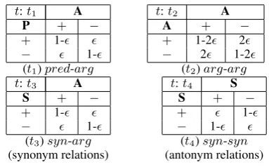
A sample instantiation of the compatibilities is shown in Table 1. Notice that the potentials forpred-arg, arg-arg, andsyn-arg capture ho-mophily, i.e., nodes with the same label are likely to connect to each other through these types of edges.4 _{On the other hand, syn-syn edges}

con-nect nodes that are antonyms of each other, and thus the compatibilities capture the reverse rela-tionship among their labels.

Table 1: Instantiation of compatibility potentials. Entry ψt

ij(yi, yj) is the compatibility of a node

with labelyi having a neighbor labeledyj, given

the edge betweeniandjis typet, for small.

t:t1 A

P + −

+ 1-

− 1-

t:t2 A

A + −

+ 1-2 2

− 2 1-2

(t1)pred-arg (t2)arg-arg t:t3 A

S + −

+ 1-

− 1-

t:t4 S

S + −

+ 1-

− 1-

(t3)syn-arg (t4)syn-syn

(synonym relations) (antonym relations)

Complexity analysis Most demanding compo-nent of Algorithm 1 is the iterative message pass-ing over the edges (lines 10-14), with time com-plexity O(ml2_{r), where m = |E| is the} num-ber of edges in the connotation graph, l = |L|, the classes, andr, the iterations until convergence. Often, l is quite small (in our case, l = 2) and

rm. Thus running time grows linearly with the number of edges and is scalable to large datasets.

4_{arg-argedges are based on co-occurrence (see Section} 2), which does not carry as strong indication of the same con-notation as e.g., synonymy. Thus, we enforce less homophily for nodes connected through edges ofarg-argtype.

4 Evaluation I: Agreement with Sentiment Lexicons

ConnotationWordNetis expected to be the super-set of a sentiment lexicon, as it is highly likely for any word with positive/negative sentiment to carry connotation of the same polarity. Thus, we use two conventional sentiment lexicons, General In-quirer (GENINQ) (Stone et al., 1966) and MPQA (Wilson et al., 2005b), as surrogates to measure the performance of our inference algorithm.

4.1 Variants of Graph Construction

The construction of the connotation graph, de-noted by GWORD+SENSE_{, which includes words and}

synsets, has been described in Section 2. In ad-dition to this graph, we tried several other graph constructions, the first three of which have previ-ously been used in (Feng et al., 2013). We briefly describe these graphs below, and compare perfor-mance on all the graphs in the proceeding.

GWORD _{W/ PRED-ARG: This is a (bipartite)}

subgraph of GWORD+SENSE_{, which only includes}

the connotative predicates and their arguments. As such, it contains only type t1 edges. The edges between the predicates and the arguments can be weighted by their Point-wise Mutual Information (PMI)5_{based on the Google Web 1T corpus.}

GWORD_{W/ OVERLAY: The second graph is also}

a proper subgraph of GWORD+SENSE_{, which}

in-cludes the predicates and all the argument words. Predicate words are connected to their arguments as before. In addition, argument pairs (a1,a2) are connected if they occurred together in the “a1 and

a2” or “a2anda1” coordination (Hatzivassiloglou and McKeown, 1997; Pickering and Branigan, 1998). This graph contains both type t1 and t2 edges. The edges can also be weighted based on the distributional similarities of the word pairs.

GWORD_{: The third graph is a super-graph of}

GWORD _{W/ OVERLAY, with additional edges,}

where argument pairs in synonym and antonym relation are connected to each other. Note that un-like the connotation graph GWORD+SENSE_{, it does}

not contain any synset nodes. Rather, the words that are synonyms or antonyms of each other are directly linked in the graph. As such, this graph contains all edge typest1throught4.

GWORD+SENSE _{W/ SYNSIM: This is a}

super-graph of our original GWORD+SENSE _{graph; that}

is, it has all the predicate, arguments, and synset nodes, as well as the four types of edges between them. In addition, we add edges of a fifth typet5 between the synset nodes to capture their similar-ity. To define similarity, we use the glossary def-initions of the synsets and derive three different scores. Each score utilizes thecount(s1, s2) of overlapping nouns, verbs, and adjectives/adverbs among the glosses of the two synsetss1 ands2.

GWORD+SENSE _{W/ SYNSIM1: We discard edges}

withcountless than 3. The weighted version has thecounts normalized between 0 and 1.

GWORD+SENSE _{W/ SYNSIM2: We normalize}

the counts by the length of the gloss (the avg of two lengths), that is, p = count /

avg(len gloss(s1), len gloss(s2))

and discard edges with p < 0.5. The weighted version containspvalues as edge weights.

GWORD+SENSE_{W/ SYNSIM3: To further sparsify}

the graph we discard edges with p < 0.6. To weigh the edges, we use the cosine similarity be-tween the gloss vectors of the synsets based on the TF-IDF values of the words the glosses contain.

Note that the connotation inference algorithm, as given in Algorithm 1, remains exactly the same for all the graphs described above. The only dif-ference is the set of parameters used; while GWORD W/ PRED-ARGand GWORD W/ OVERLAYcontain one and two edge types, respectively and only use compatibilities(t1)and(t2), GWORDuses all four as given in Table 1. The GWORD+SENSE _{W/ SYN}

-SIMgraphs use an additional compatibility matrix for the synset similarity edges of typet5, which is the same as the one used fort1, i.e., similar synsets are likely to have the same connotation label. This flexibility is one of the key advantages of our al-gorithm as new types of nodes and edges can be added to the graph seamlessly.

4.2 Sentiment-Lexicon based Performance

In this section, we first compare the performance of our connotation graph GWORD+SENSE _{to graphs}

that do not include synset nodes but only words. Then we analyze the performance when the addi-tional synset similarity edges are added. First, we briefly describe our performance measures.

The sentiment lexicons we use as gold standard are small, compared to the size (i.e., number of words) our graphs contain. Thus, we first find the overlap between each graph and a

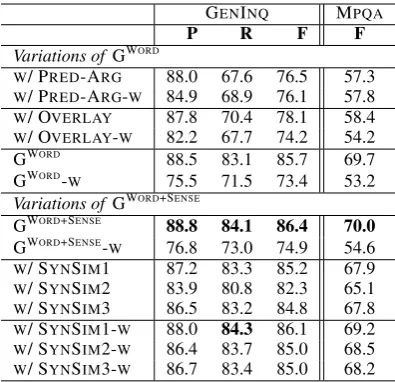
senti-GENINQ MPQA

P R F F

Variations of GWORD

W/ PRED-ARG 88.0 67.6 76.5 57.3 W/ PRED-ARG-W 84.9 68.9 76.1 57.8 W/ OVERLAY 87.8 70.4 78.1 58.4

W/ OVERLAY-W 82.2 67.7 74.2 54.2

GWORD _{88.5 83.1 85.7 69.7}

GWORD_{-W 75.5 71.5 73.4 53.2}

Variations of GWORD+SENSE

GWORD+SENSE _{88.8 84.1 86.4 70.0}

GWORD+SENSE_{-W 76.8 73.0 74.9 54.6} W/ SYNSIM1 87.2 83.3 85.2 67.9 W/ SYNSIM2 83.9 80.8 82.3 65.1 W/ SYNSIM3 86.5 83.2 84.8 67.8 W/ SYNSIM1-W 88.0 84.3 86.1 69.2

W/ SYNSIM2-W 86.4 83.7 85.0 68.5

W/ SYNSIM3-W 86.7 83.4 85.0 68.2 Table 2: Connotation inference performance on various graphs. ‘-W’ indicates weighted versions (see§4.1).P: precision,R: recall,F: F1-score (%).

ment lexicon. Note that theoverlapsize may be smaller than the lexicon size, as some sen-timent words may be missing from our graphs. Then, we calculate the number of correct la-bel assignments. As such, precision is defined as (correct/overlap), and recall as (correct

/lexicon size). Finally, F1-score is their har-monic mean and reflects the overall accuracy.

As shown in Table 2 (top), we first observe that including the synonym and antonym relations in the graph, as with GWORD _{and G}WORD+SENSE_,

im-prove the performance significantly, almost by an order of magnitude, over graphs GWORD_{W/ PRED}

-ARGand GWORD W/ OVERLAYthat do not contain those relation types. Furthermore, we notice that the performances on the GWORD+SENSE _{graph are}

better than those on the word-only graphs. This shows that including the synset nodes explicitly in the graph structure is beneficial. What is more, it gives us a means to obtain connotation labels for the synsets themselves, which we use in the evaluations in the next sections. Finally, we note that using the unweighted versions of the graphs provide relatively more robust performance, po-tentially due to noise in the relative edge weights.

Next we analyze the performance when the new edges between synsets are introduced, as given in Table 2 (bottom). We observe that connecting the synset nodes by their gloss-similarity (at least in the ways we tried) does not yield better perfor-mance than on our original GWORD+SENSE _graph.

perfor-mance than their unweighted counterparts. This suggests that glossary similarity would be a more robust means to correlate nodes; we leave it as fu-ture work to explore this direction for predicate-argument and predicate-argument-predicate-argument relations.

4.3 Parameter Sensitivity

Our belief propagation based connotation senti-ment inference algorithm has one user-specified parameter(see Table 1). To study the sensitivity of its performance to the choice of, we reran our experiments for = {0.02,0.04, . . . ,0.24}6 _and

report the accuracy results on our GWORD+SENSE_in

Figure 2 for the two lexicons. The results indicate that the performances remain quite stable across a wide range of the parameter choice.

precision recall F-score

Pe

rf

o

rma

n

ce

0 20 40 60 80 100

ε

0.02 0.06 0.10 0.14 0.18 0.22

precision recall F-score

Pe

rf

o

rma

n

ce

0 20 40 60 80 100

ε

0.02 0.06 0.10 0.14 0.18 0.22

(a) GENINQEVAL (b) MPQA EVAL Figure 2: Performance is stable across various.

5 Evaluation II: Human Evaluation on ConnotationWordNet

In this section, we present the result of human evaluation we executed using Amazon Mechani-cal Turk (AMT). We collect two separate sets of labels: a set of labels at the word-level, and an-other set at the sense-level. We first describe the labeling process of sense-level connotation: We selected 350 polysemous words and one of their senses, and each Turker was asked to rate the con-notative polarity of a given word (or of a given sense), from -5 to 5, 0 being the neutral.7_{For each}

word, we asked 5 Turkers to rate and we took the average of the 5 ratings as the connotative inten-sity score of the word. We labeled a word as nega-tiveif its intensity score is less than 0 andpositive

otherwise. For word-level labels we apply similar procedure as above.

6_{Note that for >0.25, compatibilities ofψ}t2_{in Table 1}

are reversed, hence the maximum of0.24.

7_{Because senses in WordNet can be tricky to understand,} care should be taken in designing the task so that the Turkers will focus only on the corresponding sense of a word. There-fore, we provided the part of speech tag, the WordNet gloss of the selected sense, and a few examples as given in Word-Net. As an incentive, each Turker was rewarded $0.07 per hit which consists of 10 words to label.

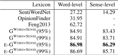
Lexicon Word-level Sense-level SentiWordNet 27.22 14.29

OpinionFinder 31.95

-Feng2013 62.72

-GWORD+SENSE_{(95%) 84.91 83.43}

GWORD+SENSE_{(99%) 84.91 83.71} E-GWORD+SENSE_{(95%) 86.98 86.29} E-GWORD+SENSE(99%) 86.69 85.71

Table 3: Word-/Sense-level evaluation results

5.1 Word-Level Evaluation

We first evaluate the word-level assignment of connotation, as shown in Table 3. The agreement between the new lexicon and human judges varies between 84% and 86.98%. Sentiment lexicons such as SentiWordNet (Baccianella et al. (2010)) and OpinionFinder (Wilson et al. (2005a)) show low agreement rate with human, which is some-what as expected: human judges in this study are labeling for subtle connotation, not for more ex-plicit sentiment. OpinionFinder’s low agreement rate was mainly due to the low hit rate of the words (successful look-up rate, 33.43%). Feng2013 is the lexicon presented in (Feng et al., 2013) and it showed a relatively higher 72.13% hit rate.

Note that belief propagation was run until 95% and 99% of the nodes were converged in their beliefs. In addition, the seed words with known connotation labels originally consist of 20 positive and 20 negative predicates. We also extended the seed set with the sentiment lexicon words and de-note these runs withE- for ‘Extended’.

5.2 Sense-Level Evaluation

We also examined the agreement rates on the sense-level. Since OpinionFinder and Feng2013 do not provide the polarity scores at the sense-level, we excluded them from this evaluation. Be-cause sense-level polarity assignment is a harder (more subtle) task, the performance of all lexicons decreased to some degree in comparison to that of word-level evaluations.

5.3 Pair-wise Intensity Ranking

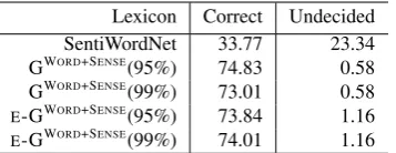
Lexicon Correct Undecided SentiWordNet 33.77 23.34 GWORD+SENSE_{(95%) 74.83 0.58}

GWORD+SENSE_{(99%) 73.01 0.58} E-GWORD+SENSE_{(95%) 73.84 1.16} E-GWORD+SENSE(99%) 74.01 1.16

Table 4: Results of pair-wise intensity evaluation, for intensity difference threshold = 2.0

already have this information at hand. Because different human judges have different notion of scales however, subtle differences are more likely to be noisy. Therefore, we experiment with vary-ing degrees of differences in their scales, as shown in Figure 3. Threshold values (ranging from 0.5 to 3.0) indicate the minimum differences in scales for any pair of words, for the pair to be included in the test set. As expected, we observe that the perfor-mance improves as we increase the threshold (as pairs get better separated). Within range [0.5, 1.5] (249 pairs examined), the accuracies are as high as 68.27%, which shows that even the subtle differ-ences of the connotative intensities are relatively well reflected in the new lexicons.

SentiWordNet GWord+Sense(95%) GWord+Sense_(99%) e-GWord+Sense(95%) e-GWord+Sense(99%)

Accu

ra

cy

(%

)

40 60 80

Threshold

0.5 1.0 2.0 3.0

Figure 3: Trend of accuracy for pair-wise intensity evaluation over threshold

The results for pair-wise intensity evaluation (threshold=2.0, 1,208 pairs) are given in Table 4. Despite that intensity is generally a harder prop-erty to measure (than the coarser binary catego-rization of polarities), our connotation lexicons perform surprisingly well, reaching up to 74.83% accuracy. Further study on the incorrect cases re-veals that SentiWordNet has many pair of words with the same polarity score (23.34%). Such cases seems to be due to the limited score patterns of SentiWordNet. The ratio of such cases are ac-counted asUndecidedin Table 4.

6 Evaluation III: Sentiment Analysis using ConnotationWordNet

Finally, to show the utility of the resulting lexi-con in the lexi-context of a lexi-concrete sentiment analysis

task, we perform lexicon-based sentiment analy-sis. We experiment with SemEval dataset (Strap-parava and Mihalcea, 2007) that includes the hu-man labeled dataset for predicting whether a news headline is agood newsor abad news, which we expect to have a correlation with the use of con-notativewords that we focus on in this paper. The good/bad news are annotated with scores (ranging from -100 to 87). We construct several data sets by applying different thresholds on scores. For exam-ple, with the threshold set to 60, we discard the in-stances whose scores lie between -60 and 60. For comparison, we also test the connotation lexicon from (Feng et al., 2013) and the combined senti-ment lexicon GENINQ+MPQA.

Note that there is a difference in how humans judge the orientation and the degree of connota-tion for a given word out of context, and how the use of such words in context can be perceived as

good/bad news. In particular, we conjecture that humans may have a bias toward the use of posi-tive words, which in turn requires calibration from the readers’ minds (Pennebaker and Stone, 2003). That is, we might need to tone down the level of positiveness in order to correctly measure the ac-tual intended positiveness of the message.

With this in mind, we tune the appropriate cali-bration from a small training data, by using 1 fold from N fold cross validation, and using the re-mainingN −1folds as testing. We simply learn the mixture coefficientλto scale the contribution of positive and negative connotation values. We tune this parameterλ8_{for other lexicons we}

com-pare against as well. Note that due to this param-eter learning, we are able to report better perfor-mance for the connotation lexicon of (Feng et al., 2013) than what the authors have reported in their paper (labeled with *) in Table 5.

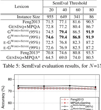
Table 5 shows the results for N=15, where the new lexicon consistently outperforms other com-petitive lexicons. In addition, Figure 4 shows that the performance does not change much based on the size of training data used for parameter tuning (N={5,10,15,20}).

7 Related Work

Lexicon SemEval Threshold

20 40 60 80

Instance Size 955 649 341 86 Feng2013 71.5 77.1 81.6 90.5 GENINQ+MPQA 72.8 77.2 80.4 86.7

GWORD+SENSE_{(95%) 74.5 79.4 86.5 91.9}

GWORD+SENSE_{(99%) 74.6 79.4 86.8 91.9} E-GWORD+SENSE_{(95%) 72.5 76.8 82.3 87.2} E-GWORD+SENSE_{(99%) 72.6 76.9 82.5 87.2}

Feng2013* 70.8 74.6 80.8 93.5 GENINQ+MPQA* 64.5 69.0 74.0 80.5

Table 5: SemEval evaluation results, forN=15

Feng2013 MPQA+GenInq GWord+Sense(95%) GWord+Sense(99%) e-GWord+Sense_(95%)

e-GWord+Sense(99%)

Accu

ra

cy

(%

)

50 60 70 80

N

5 10 15 20

Figure 4: Trend of SemEval performance overN, the number of CV folds

induction (Feng et al., 2013). Our work intro-duces the use of loopy belief propagation over pairwise-MRF as an alternative solution to these tasks. At a high-level, both approaches share the general idea of propagating confidence or belief over the graph connectivity. The key difference, however, is that in our MRF representation, we can explicitly model various types of word-word, sense-sense and word-sense relations as edge po-tentials. In particular, we can naturally encode re-lations that encourage the same assignment (e.g., synonym) as well as the opposite assignment (e.g., antonym) of the polarity labels. Note that integra-tion of the latter is not straightforward in the graph propagation framework.

There have been a number of previous studies that aim to construct a word-level sentiment lex-icon (Wiebe et al., 2005; Qiu et al., 2009) and a sense-level sentiment lexicon (Esuli and Sebas-tiani, 2006). But none of these approaches con-sidered to induce the polarity labels at both the word-level and sense-level. Although we focus on learning connotative polarity of words and senses in this paper, the same approach would be applica-ble to constructing a sentiment lexicon as well.

There have been recent studies that address word sense disambiguation issues for sentiment analysis. SentiWordNet (Esuli and Sebastiani, 2006) was the very first lexicon developed for

sense-level labels of sentiment polarity. In recent years, Akkaya et al. (2009) report a successful em-pirical result where WSD helps improving senti-ment analysis, while Wiebe and Mihalcea (2006) study the distinction between objectivity and sub-jectivity in each different sense of a word, and their empirical effects in the context of sentiment analysis. Our work shares the high-level spirit of accessing the sense-level polarity, while also de-riving the word-level polarity.

In recent years, there has been a growing re-search interest in investigating more fine-grained aspects of lexical sentiment beyond positive and negative sentiment. For example, Mohammad and Turney (2010) study the affects words canevoke

in people’s minds, while Bollen et al. (2011) study various moods, e.g., “tension”, “depression”, be-yond simple dichotomy of positive and negative sentiment. Our work, and some recent work by Feng et al. (2011) and Feng et al. (2013) share this spirit by targeting more subtle, nuanced sentiment even from those words that would be considered as objective in early studies of sentiment analysis.

8 Conclusion

We have introduced a novel formulation of lexicon induction operating over both words and senses, by exploiting the innate structure between the words and senses as encoded in WordNet. In addi-tion, we introduce the use of loopy belief propaga-tion over pairwise-Markov Random Fields as an effective lexicon induction algorithm. A notable strength of our approach is its expressiveness: var-ious types of prior knowledge and lexical relations can be encoded as node potentials and edge po-tentials. In addition, it leads to a lexicon of bet-ter quality while also offering fasbet-ter run-time and easiness of implementation. The resulting lexi-con, called ConnotationWordNet, is the first lex-icon that has polarity labels over both words and senses. ConnotationWordNetis publicly available for research and practical use.

Acknowledgments

References

Cem Akkaya, Janyce Wiebe, and Rada Mihalcea. 2009. Subjectivity word sense disambiguation. In

Proceedings of the 2009 Conference on Empirical Methods in Natural Language Processing: Volume 1-Volume 1, pages 190–199. Association for Com-putational Linguistics.

Leman Akoglu, Rishi Chandy, and Christos Faloutsos. 2013. Opinion fraud detection in online reviews by network effects.

Alina Andreevskaia and Sabine Bergler. 2006. Min-ing wordnet for a fuzzy sentiment: Sentiment tag extraction from wordnet glosses. In EACL, pages 209–216.

Stefano Baccianella, Andrea Esuli, and Fabrizio Sebas-tiani. 2010. Sentiwordnet 3.0: An enhanced lexical resource for sentiment analysis and opinion mining. InLREC, volume 10, pages 2200–2204.

Alexandra Balahur, Rada Mihalcea, and Andr´es Mon-toyo. 2014. Computational approaches to subjec-tivity and sentiment analysis: Present and envisaged methods and applications. Computer Speech & Lan-guage, 28(1):1–6.

Johan Bollen, Huina Mao, and Alberto Pepe. 2011. Modeling public mood and emotion: Twitter senti-ment and socio-economic phenomena. InICWSM.

K. W. Church and P. Hanks. 1990. Word association norms, mutual information, and lexicography. Com-putational Linguistics, 1(16):22–29.

Andrea Esuli and Fabrizio Sebastiani. 2006. Sen-tiwordnet: A publicly available lexical resource for opinion mining. In In Proceedings of the 5th Conference on Language Resources and Evaluation (LREC06, pages 417–422.

Song Feng, Ritwik Bose, and Yejin Choi. 2011. Learn-ing general connotation of words usLearn-ing graph-based algorithms. In Proceedings of the Conference on Empirical Methods in Natural Language Process-ing, pages 1092–1103. Association for Computa-tional Linguistics.

Song Feng, Jun Seok Kang, Polina Kuznetsova, and Yejin Choi. 2013. Connotation lexicon: A dash of sentiment beneath the surface meaning. In The Association for Computer Linguistics, pages 1774– 1784.

Vasileios Hatzivassiloglou and Kathleen McKeown. 1997. Predicting the semantic orientation of adjec-tives. InProceedings of the Joint ACL/EACL Con-ference, pages 174–181.

Nobuhiro Kaji and Masaru Kitsuregawa. 2007. Build-ing lexicon for sentiment analysis from massive col-lection of html documents. In EMNLP-CoNLL, pages 1075–1083.

Jaap Kamps, MJ Marx, Robert J Mokken, and Maarten De Rijke. 2004. Using wordnet to measure seman-tic orientations of adjectives.

Ross Kindermann and J. L. Snell. 1980. Markov Ran-dom Fields and Their Applications.

Yue Lu, Malu Castellanos, Umeshwar Dayal, and ChengXiang Zhai. 2011. Automatic construction of a context-aware sentiment lexicon: an optimiza-tion approach. InProceedings of the 20th interna-tional conference on World wide web, pages 347– 356. ACM.

Mary McGlohon, Stephen Bay, Markus G. Anderle, David M. Steier, and Christos Faloutsos. 2009. Snare: a link analytic system for graph labeling and risk detection. In John F. Elder IV, Franoise Fogelman-Souli, Peter A. Flach, and Mohammed Zaki, editors,KDD, pages 1265–1274. ACM.

Rada Mihalcea, Carmen Banea, and Janyce Wiebe. 2012. Multilingual subjectivity and sentiment anal-ysis. InTutorial Abstracts of ACL 2012, pages 4–4. Association for Computational Linguistics.

Saif Mohammad and Peter Turney. 2010. Emotions evoked by common words and phrases: Using me-chanical turk to create an emotion lexicon. In Pro-ceedings of the NAACL HLT 2010 Workshop on Computational Approaches to Analysis and Genera-tion of EmoGenera-tion in Text, pages 26–34, Los Angeles, CA, June. Association for Computational Linguis-tics.

David Newman, Sarvnaz Karimi, and Lawrence Cave-don. 2009. External evaluation of topic models. In Australasian Document Computing Symposium, pages 11–18, Sydney, December.

Shashank Pandit, Duen Horng Chau, Samuel Wang, and Christos Faloutsos. 2007. Netprobe: a fast and scalable system for fraud detection in online auction networks. InWWW, pages 201–210.

Christos H Papadimitriou and Kenneth Steiglitz. 1998.

Combinatorial optimization: algorithms and com-plexity. Courier Dover Publications.

James W Pennebaker and Lori D Stone. 2003. Words of wisdom: language use over the life span.Journal of personality and social psychology, 85(2):291.

John P Pestian, Pawel Matykiewicz, Michelle Linn-Gust, Brett South, Ozlem Uzuner, Jan Wiebe, K Bre-tonnel Cohen, John Hurdle, Christopher Brew, et al. 2012. Sentiment analysis of suicide notes: A shared task. Biomedical Informatics Insights, 5(Suppl. 1):3.

Guang Qiu, Bing Liu, Jiajun Bu, and Chun Chen. 2009. Expanding domain sentiment lexicon through double propagation. In IJCAI, volume 9, pages 1199–1204.

Prithviraj Sen, Galileo Namata, Mustafa Bilgic, Lise Getoor, Brian Gallagher, and Tina Eliassi-Rad. 2008. Collective classification in network data. AI Magazine, 29(3):93–106.

Philip J. Stone, Dexter C. Dunphy, Marshall S. Smith, and Daniel M. Ogilvie. 1966. The General In-quirer: A Computer Approach to Content Analysis. MIT Press, Cambridge, MA.

Carlo Strapparava and Rada Mihalcea. 2007. Semeval-2007 task 14: Affective text. In Proceedings of the 4th International Workshop on Semantic Evalu-ations, pages 70–74. Association for Computational Linguistics.

Fangzhong Su and Katja Markert. 2009. Subjectiv-ity recognition on word senses via semi-supervised mincuts. InProceedings of Human Language Tech-nologies: The 2009 Annual Conference of the North American Chapter of the Association for Computa-tional Linguistics, pages 1–9. Association for Com-putational Linguistics.

Hiroya Takamura, Takashi Inui, and Manabu Okumura. 2005. Extracting semantic orientations of words us-ing spin model. InProceedings of the 43rd Annual Meeting on Association for Computational Linguis-tics, pages 133–140. Association for Computational Linguistics.

Peter D. Turney. 2001. Mining the Web for synonyms: PMI-IR versus LSA on TOEFL. In Proceedings of the Twelfth European Conference on Machine Learning (ECML-01), pages 491–502, Freiburg, Germany.

Leonid Velikovich, Sasha Blair-Goldensohn, Kerry Hannan, and Ryan McDonald. 2010. The via-bility of web-derived polarity lexicons. InHuman Language Technologies: The 2010 Annual Confer-ence of the North American Chapter of the Associa-tion for ComputaAssocia-tional Linguistics. Association for Computational Linguistics.

Janyce Wiebe and Rada Mihalcea. 2006. Word sense and subjectivity. In Proceedings of the 21st Inter-national Conference on Computational Linguistics and the 44th annual meeting of the Association for Computational Linguistics, pages 1065–1072. Asso-ciation for Computational Linguistics.

Janyce Wiebe, Theresa Wilson, and Claire Cardie. 2005. Annotating expressions of opinions and emo-tions in language. Language Resources and Eval-uation (formerly Computers and the Humanities), 39(2/3):164–210.

Theresa Wilson, Paul Hoffmann, Swapna Somasun-daran, Jason Kessler, Janyce Wiebe, Yejin Choi,

Claire Cardie, Ellen Riloff, and Siddharth Patward-han. 2005a. Opinionfinder: A system for subjec-tivity analysis. InProceedings of HLT/EMNLP on Interactive Demonstrations, pages 34–35. Associa-tion for ComputaAssocia-tional Linguistics.

Theresa Wilson, Janyce Wiebe, and Paul Hoffmann. 2005b. Recognizing contextual polarity in phrase-level sentiment analysis. InProceedings of Human Language Technologies Conference/Conference on Empirical Methods in Natural Language Processing (HLT/EMNLP 2005), Vancouver, CA.