Heuristic Cube Pruning in Linear Time
Andrea Gesmundo
Department of Computer Science University of Geneva
Giorgio Satta
Department of Information Engineering
University of Padua
James Henderson
Department of Computer Science University of Geneva
Abstract
We propose a novel heuristic algorithm for Cube Pruning running in linear time in the beam size. Empirically, we show a gain in running time of a standard machine translation system, at a small loss in accuracy.
1 Introduction
Since its first appearance in (Huang and Chiang, 2005), the Cube Pruning (CP) algorithm has quickly gained popularity in statistical natural language pro-cessing. Informally, this algorithm applies to sce-narios in which we have thek-best solutions for two input sub-problems, and we need to compute thek -best solutions for the new problem representing the combination of the two sub-problems.
CP has applications in tree and phrase based ma-chine translation (Chiang, 2007; Huang and Chi-ang, 2007; Pust and Knight, 2009), parsing (Huang and Chiang, 2005), sentence alignment (Riesa and Marcu, 2010), and in general in all systems combin-ing inexact beam decodcombin-ing with dynamic program-ming under certain monotonic conditions on the def-inition of the scores in the search space.
Standard implementations of CP run in time
O(klog(k)), with k being the size of the in-put/output beams (Huang and Chiang, 2005). Ges-mundo and Henderson (2010) propose Faster CP (FCP) which optimizes the algorithm but keeps the
O(klog(k))time complexity. Here, we propose a novel heuristic algorithm for CP running in time
O(k) and evaluate its impact on the efficiency and performance of a real-world machine translation system.
2 Preliminaries
LetL = hx0, . . . , xk−1i be a list over R, that is, an ordered sequence of real numbers, possibly with repetitions. We write|L|=kto denote the length of
L. We say thatLis descending ifxi ≥xjfor every i, j with0 ≤i < j < k. LetL1 = hx0, . . . , xk−1i and L2 = hy0, . . . , yk′−1i be two descending lists overR. We writeL1⊕ L2to denote the descending list with elementsxi+yjfor everyi, jwith0≤i < kand0≤j < k′.
In cube pruning (CP) we are given as input two descending listsL1,L2 overRwith|L1| =|L2| =
k, and we are asked to compute the descending list consisting of the firstkelements ofL1⊕ L2.
A problem related to CP is the k-way merge problem (Horowitz and Sahni, 1983). Given de-scending lists Li for every iwith 0 ≤ i < k, we
writemergek−1
i=0 Li to denote the “merge” of all the
listsLi, that is, the descending list with all elements
from the listsLi, including repetitions.
For∆ ∈Rwe defineshift(L,∆) =L ⊕ h∆i. In words,shift(L,∆)is the descending list whose ele-ments are obtained by “shifting” the eleele-ments ofL
by∆, preserving the order. LetL1,L2 be descend-ing lists of length k, with L2 = hy0, . . . , yk−1i. Then we can express the output of CP onL1,L2 as the list
mergek−1
i=0 shift(L1, yi) (1)
truncated after the firstkelements. This shows that the CP problem is a particular instance of thek-way merge problem, in which all input lists are related by
kindependent shifts.
Computation of the solution of thek-way merge problem takes time O(qlog(k)), where q is the size of the output list. In case each input list has lengthkthis becomesO(k2
log(k)), and by restrict-ing the computation to the firstk elements, as re-quired by the CP problem, we can further reduce to
O(klog(k)). This is the already known upper bound on the CP problem (Huang and Chiang, 2005; Ges-mundo and Henderson, 2010). Unfortunately, there seems to be no way to achieve an asymptotically faster algorithm by exploiting the restriction that the input lists are all related by some shifts. Nonethe-less, in the next sections we use the above ideas to develop a heuristic algorithm running in time linear ink.
3 Cube Pruning With Constant Slope
Consider listsL1,L2defined as in section 2. We say thatL2has constant slope ifyi−1−yi= ∆>0for
everyiwith0< i < k. Throughout this section we assume thatL2 has constant slope, and we develop an (exact) linear time algorithm for solving the CP problem under this assumption.
For each i ≥ 0, let Ii be the left-open interval (x0−(i+ 1)·∆, x0 −i·∆]ofR. Let also s =
⌊(x0 −xk−1)/∆⌋+ 1. We split L1 into (possibly empty) sublistsσi,0≤i < s, called segments, such
that eachσi is the descending sublist consisting of
all elements fromL1that belong toIi. Thus, moving
down one segment inL1 is the closest equivalent to moving down one element inL2.
Let t = min{k, s}; we define descending lists
Mi, 0 ≤ i < t, as follows. We set M0 =
shift(σ0, y0), and for1≤i < twe let
Mi=merge{shift(σi, y0),shift(Mi−1,−∆)} (2)
We claim that the ordered concatenation of M0,
M1, . . . , Mt−1 truncated after the first k elements is exactly the output of CP on inputL1,L2.
To prove our claim, it helps to visualize the de-scending listL1⊕ L2(of sizek2) as ak×kmatrix
Lwhose j-th column is shift(L1, yj), 0 ≤ j < k.
For an intervalI = (x, x′], we define shift(I, y) = (x+y, x′+y]. Similarly to what we have done with L1, we can split each column ofLintossegments. For eachi, j with0≤i < sand0≤j < k, we de-fine thei-th segment of thej-th column, writtenσi,j,
as the descending sublist consisting of all elements of that column that belong toshift(Ii, yj). Then we
haveσi,j =shift(σi, yj).
For any d with 0 ≤ d < t, consider now all segments σi,j with i + j = d, forming a
sub-antidiagonal inL. We observe that these segments contain all and only those elements ofLthat belong to the interval Id. It is not difficult to show by
in-duction that these elements are exactly the elements that appear in descending order in the listMidefined
in (2).
We can then directly use relation (2) to iteratively compute CP on two lists of lengthk, under our as-sumption that one of the two lists has constant slope. Using the fact that the merge of two lists as in (2) can be computed in time linear in the size of the output list, it is not difficult to implement the above algo-rithm to run in timeO(k).
4 Linear Time Heuristic Solution
In this section we further elaborate on the exact al-gorithm of section 3 for the constant slope case, and develop a heuristic solution for the general CP prob-lem. LetL1,L2, Landkbe defined as in sections 2 and 3. Despite the fact thatL2does not have a con-stant slope, we can still split each column ofLinto segments, as follows.
LetIei,0 ≤ i < k −1, be the left-open interval (x0+yi+1, x0+yi]ofR. Note that, unlike the case
of section 3, intervalsIei’s are not all of the same size
now. Let alsoIek−1 = [xk−1 +yk−1, x0+yk−1]. For eachi, j with0 ≤ j < k and 0 ≤ i < k − j, we define segmentσei,j as the descending sublist
consisting of all elements of thej-th column ofL
that belong to Iei+j. In this way, the j-th column
of Lis split into segments Iej, Iej+1, . . . , Iek−1, and we have a variable number of segments per column. Note that segmentseσi,jwith a constant value ofi+j
contain all and only those elements ofLthat belong to the left-open intervalIei+j.
Similarly to section 3, we define descending lists
f
Mi, 0 ≤ i < k, by setting Mf0 = eσ0,0 and, for
1≤i < k, by letting
f
Mi =merge{eσi,0, path(Mfi−1, L)} (3)
1: Algorithm 1 (L1,L2) :Le⋆ 2: Le⋆.insert(L[0,0]);
3: referColumn←0; 4: xfollow ←L[0,1]; 5: xdeviate ←L[1,0]; 6: C ←CircularList([0,1]); 7: C-iterator← C.begin(); 8: while|Le⋆|< kdo
9: ifxfollow > xdeviatethen
10: Le⋆.insert(xfollow);
11: ifC-iterator.current()=[0,1]then
12: referColumn++; 13: [i, j]← C-iterator.next(); 14: xfollow ←L[i,referColumn+j]; 15: else
16: Le⋆.insert(xdeviate); 17: i←xdeviate.row();
18: C-iterator.insert([i,−referColumn]); 19: xdeviate ←L[i+ 1,0];
case of (2). This is because input listL2 does not have constant slope in general. In an exact algo-rithm,path(Mfi−1, L)should return the descending listL⋆
i−1 =mergeij=1 eσi−j,j: Unfortunately, we do
not know how to compute such ai-way merge with-out introducing a logarithmic factor.
Our solution is to definepath(Mfi−1, L)in such a way that it computes a listLei−1 which is a permu-tation of the correct solutionL⋆
i−1. To do this, we consider the “relative” path starting atx0+yi−1that we need to follow inLin order to collect all the el-ements ofMfi−1 in the given order. We then apply such a path starting atx0+yiand return the list of
collected elements. Finally, we compute the output listLe⋆ as the concatenation of all listsMf
i up to the
firstkelements.
It is not difficult to see that whenL2has constant slope we haveMfi = Mi for alliwith0 ≤i < k,
and list Le⋆ is the exact solution to the CP
prob-lem. WhenL2 does not have a constant slope, list
e
L⋆ might depart from the exact solution in two
[image:3.612.314.539.62.274.2]re-spects: it might not be a descending list, because of local variations in the ordering of the elements; and it might not be a permutation of the exact so-lution, because of local variations at the end of the list. In the next section we evaluate the impact that
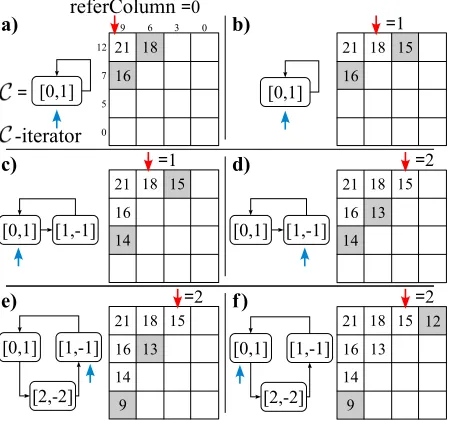
Figure 1: A running example for Algorithm 1.
our heuristic solution has on the performance of a real-world machine translation system.
Algorithm 1 implements the idea presented in (3). The algorithm takes as input two descending lists
L1,L2 of length k and outputs the list Le⋆ which approximates the desired solution. ElementL[i, j]
denotes the combined valuexi +yj, and is always
computed on demand.
We encode a relative path (mentioned above) as a sequence of elements, called displacements, each of the form[i, δ]. Hereiis the index of the next row, andδrepresents the relative displacement needed to reach the next column, to be summed to a variable called referColumn denoting the index of the col-umn of the first element of the path. The reason why only the second coordinate is a relative value is that we shift paths only horizontally (row indices are preserved). The relative path is stored in a circu-lar listC, with displacement[0,1]marking the start-ing point (paths are always shifted one element to the right). When merging the list obtained through the path for Mfi−1 with segment eσi,0, as specified in (3), we updateCaccordingly, so that the new rel-ative path can be used at the next round forMfi. The
-5 0 5 10 15 20 25 30 35 40 45
1 10 100 1000
score loss (%)
beam size
[image:4.612.315.533.61.215.2]Baseline score loss over CP LCP score loss over CP FCP score loss over CP
Figure 2: Search-score loss relative to standard CP.
else depart visiting an element fromσei,0in the first column ofL(lines 16 to 19). In the latter case, we updateCwith the new displacement (line 18), where the function insert() inserts a new element before the one currently pointed to. The function next() at line 13 moves the iterator to the next element and then returns its value.
A running example of algorithm 1 is reported in Figure 1. The input lists are L1 = h12,7,5,0i,
L2=h9,6,3,0i. Each of the picture in the sequence represents the state of the algorithm when the test at line 9 is executed. The value in the shaded cell in the first column isxdeviate, while the value in the other shaded cell isxfollow.
5 Experiments
We implement Linear CP (LCP) on top of Cdec (Dyer et al., 2010), a widely-used hierarchical MT system that includes implementations of standard CP and FCP algorithms. The experiments were ex-ecuted on the NIST 2003 Chinese-English parallel corpus. The training corpus contains 239k sentence pairs. A binary translation grammar was extracted using a suffix array rule extractor (Lopez, 2007). The model was tuned using MERT (Och, 2003). The algorithms are compared on the NIST-03 test set, which contains 919 sentence pairs. The features used are basic lexical features, word penalty and a 3-gram Language Model (Heafield, 2011).
Since we compare decoding algorithms on the same search space, the accuracy comparison is done in terms of search score. For each algorithm we
0 5 10 15 20 25
1 10 100 1000
speed gain (%)
beam size
LCP speed gain over CP LCP speed gain over FCP
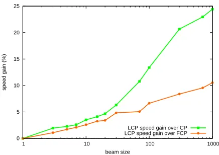
Figure 3: Linear CP relative speed gain.
compute the average score of the best translation found for the test sentences. In Figure 2 we plot the score-loss relative to standard CP average score. Note that the FCP loss is always<3%, and the LCP loss is always<7%. The dotted line plots the loss of a baseline linear time heuristic algorithm which assumes that both input lists have constant slope, and that scans L along parallel lines whose steep is the ratio of the average slope of each input list. The baseline greatly deteriorates the accuracy: this shows that finding a reasonable linear time heuristic algorithm is not trivial. We can assume a bounded loss in accuracy, because for larger beam size all the algorithms tend to converge to exhaustive search.
We found that these differences in search score resulted in no significant variations in BLEU score (e.g. withk = 30, CP reaches 32.2 while LCP 32.3). The speed comparison is done in terms of algo-rithm run-time. Figure 3 plots the relative speed gain of LCP over standard CP and over FCP. Given the log-scale used for the beam sizek, the linear shape of the speed gain over FCP (and CP) in Figure 3 em-pirically confirms that LCP has alog(k)asymptotic advantage over FCP and CP.
In addition to Chinese-English, we ran experi-ments on translating English to French (from Eu-roparl corpus (Koehn, 2005)), and find that the LCP score-loss relative to CP is< 9%while the speed relative advantage of LCP over CP increases in aver-age by11.4%every time the beam size is multiplied by10 (e.g. with k = 1000 the speed advantage is
[image:4.612.77.296.63.215.2]References
David Chiang. 2007. Hierarchical phrase-based transla-tion. Computational Linguistics, 33(2):201–228. Chris Dyer, Adam Lopez, Juri Ganitkevitch, Jonathan
Weese, Hendra Setiawan, Ferhan Ture, Vladimir Ei-delman, Phil Blunsom, and Philip Resnik. 2010. cdec: A decoder, alignment, and learning framework for finite-state and context-free translation models. In ACL ’10: Proceedings of the ACL 2010 System
Demonstrations, Uppsala, Sweden.
Andrea Gesmundo and James Henderson. 2010. Faster Cube Pruning. In IWSLT ’10: Proceedings of the 7th
International Workshop on Spoken Language Transla-tion, Paris, France.
Kenneth Heafield. 2011. KenLM: Faster and smaller language model queries. In WMT ’11: Proceedings of
the 6th Workshop on Statistical Machine Translation,
Edinburgh, Scotland, UK.
E. Horowitz and S. Sahni. 1983. Fundamentals of data structures. Computer software engineering
se-ries. Computer Science Press.
Liang Huang and David Chiang. 2005. Better k-best parsing. In IWPT ’05: Proceedings of the 9th
Interna-tional Workshop on Parsing Technology, Vancouver,
British Columbia, Canada.
Liang Huang and David Chiang. 2007. Forest rescor-ing: Faster decoding with integrated language mod-els. In ACL ’07: Proceedings of the 45th
Confer-ence of the Association for Computational Linguistics,
Prague, Czech Republic.
Philipp Koehn. 2005. Europarl: A parallel corpus for statistical machine translation. In Proceedings of the
10th Machine Translation Summit, Phuket, Thailand.
Adam Lopez. 2007. Hierarchical phrase-based transla-tion with suffix arrays. In EMNLP-CoNLL ’07:
Pro-ceedings of the 2007 Joint Conference on Empirical Methods in Natural Language Processing and Com-putational Natural Language Learning, Prague, Czech
Republic.
Franz Josef Och. 2003. Minimum error rate training in statistical machine translation. In ACL ’03:
Pro-ceedings of the 41st Conference of the Association for Computational Linguistics, Sapporo, Japan.
Michael Pust and Kevin Knight. 2009. Faster MT decod-ing through pervasive laziness. In NAACL ’09:
Pro-ceedings of the 10th Conference of the North American Chapter of the Association for Computational Linguis-tics, Boulder, CO, USA.
Jason Riesa and Daniel Marcu. 2010. Hierarchical search for word alignment. In ACL ’10: Proceedings