Application of a Tritium Imaging Plate Technique to Depth Profiling of Hydrogen in
Metals and Determination of Hydrogen Diffusion Coefficients
Teppei Otsuka
1,*and Tetsuo Tanabe
21Department of Electric and Electronic Engineering, Faculty of Science and Engineering, Kindai University,
Higashi-Osaka 577–8502, Japan
2Interdisciplinary Graduate school of Engineering Sciences, Kyushu University, Kasuga 816–8580, Japan
A new methodology for depth profiling of hydrogen in metals is developed applying a tritium imaging plate technique (TIPT) with cross sectional observation. Owing to its high sensitivity and wide dynamic range for tritium detection, depth distribution of hydrogen dissolved in the BCC metals such as tungsten (W) and steels are successfully obtained. The depth distributions enable us to determine reliable lattice diffu-sion coefficients of hydrogen in W and a ferritic/martensitic steel (F82H) within 20% errors taking into account three dimensional desorption/ release from the surfaces of the sample metals. Hydrogen trapped at surface and subsurface are clearly separated from the dissolved one. In BCC metals, since the former could be much larger than the latter, observation of overall hydrogen behavior without knowing detailed depth distributions could lead to wrong estimation of diffusion coefficients and solubility. [doi:10.2320/matertrans.M2017175]
(Received June 14, 2017; Accepted July 21, 2017; Published September 25, 2017)
Keywords: hydrogen, tritium, tungsten, ferritic steel, imaging plate, depth profile, diffusion coefficient, trapping
1. Introduction
Hydrogen (H) diffusion coefficients in metals have been determined mostly by permeation or desorption, owing to easy detection of permeated or desorbed hydrogen. However, permeation and desorption are often disturbed by trapping effects, resulting in significant reduction of appar-ent diffusion coefficiappar-ents. The trapping effects are apprecia-ble particularly in BCC metals like iron (Fe) and tungsten
(W)1,2) in which H solubility is much less than that of FCC
metals like nickel (Ni). Furthermore, a tiny H flux permeated or desorbed from the metals surfaces are easily affected by surface impurities like oxygen (O) and carbon (C), which are segregated from bulk or taken from surrounding atmo-sphere; even H2 gas includes H2O3). In order to avoid the
ef-fects of trapping and surface impurities, diffusion analysis based on depth distribution would be better compared to those based on H release.
However, observation of H depth distribution in metals is quite hard. Although various ion beam techniques give the H depth distribution, they are limited in near surface region. Only a sectioning method allows us to determine the H depth distribution, in which a H loaded sample is sectioned into small pieces parallel to the sample surface toward a depth direction and H retained in the sectioned pieces is de-termined by thermal desorption or other H detection tech-niques. Several problems still remain in the sectioning method; time consuming for the sectioning process accom-panying possible H release, difficulty of detection of small amount of H, and very poor depth resolution. Applying a tri-tium (T) tracer technique, diffusional behaviors of T diluted in H in hydride forming metals have been investigated by
the sectioning method4,5). However, metals which absorb H
endothermically, such as Fe and W (referred as endothermic H occluders, hereafter) having very low solubility, were quite hard to observe the H depth distribution by the
time-consuming sectioning method.
In previous studies, we have applied a tritium imaging plate technique (TIPT) to get H depth distributions in mm to
cm scale in depth with a depth resolution of several tens μm
by a cross-sectioning method. In this method, a T loaded sample was bisected perpendicular to the loaded surface to appear a cross-sectional surface and an areal T distribution on the surface (T profile) was observed by TIPT. With this method, we have succeeded to get reliable depth distribu-tions of H (T) loaded in hydride forming metals like
zirco-nium and vanadium alloys6–10). In the present study, we have
established TIPT to observe T surface profile and depth dis-tribution with the cross-sectioning method and successfully applied to investigate solution, trapping, diffusion and
de-sorption/permeation behaviors of H in endothermic
hydro-gen occluders of pure W11) and a ferritic/martensitic
steel12,13) which are candidates of plasma facing wall and/or
a structure in a nuclear fusion reactor.
2. Principle of Tritium Imaging Plate Technique (TIPT)
Quantification of the absolute amount of T in metals by radiation measurements is not easy because energy of
emit-ted electrons by β-decay of T (hereinafter referred as T
β-electrons) is too low to pass through materials (even in air) in a long distance. TIPT is a good method to detect T exist-ing on metal s surface and have been used for surface profil-ing of T. Nevertheless, to quantify T concentration with the
detection of the T β-electrons by TIPT, their energy loss
during passing through materials before coming in a detec-tor (IP) should be taken into account.
This section describes how the T β-electrons lose their
en-ergy during passing through a metal and deposit their re-maining energy on IP attached to the surface of the metal.
2.1 Detection of β-electrons emitted from the surface of metals retaining T
When an electron having energy is emitted by β-decay
of a T atom in a material and travels in it to the z direction, it loses energy as,
−∂z =S( ), (1)
where S( ) is referred as a stopping power (eV·m−1), which
is determined experimentally and/or theoretically. When the
electron comes up to the surface after travelling distance z in a material with its initial energy 0 , its energy is reduced to
(z)= 0− z
0
(S ( ))dz. (2)
The energy of the β-electron ranges from 0 to 18.6 keV
with the average of 5.7 keV. When T atoms are distributed in depth with their areal density of ρ(z), they emit β-electrons
with areal energy density of λρ(z) in a unit time. Here λ
(s−1) is the disintegration constant of T. Then energy flux
carried by escaping electrons from the surface is given by,
=
z
0
18.6keV
0 0−
z
0 (S ( )) λρ(z)d dz. (3) When an imaging plate (IP) made of a plastic substrate
coated with phosphor layers (BaFBr:Eu2+) contacts to the
surface of the metal retaining T for a certain time duration, all emitted energy given by eq. (3) is absorbed (deposited) in the phosphor layers, since their thickness is enough to stop all electrons escaping from the surface. Certain parts of the deposited energy in IP is used to excite electrons in the phosphors from the ground state to an quasi-stable exited
state14). When the excited electrons are further excited to a
little higher energy level by violet photons, they are relaxed with photon emission referred as Photo-Stimulated Luminescence (PSL). An IP reader makes this process to give digitized PSL intensity from IP exposed to a T retaining sample. The PSL intensity shows a good linear relationship with the deposited energy in IP over five orders of magni-tude. Then the deposited energy profile determined from the PSL intensity profile is correlated to a T depth distribution,
ρ(z), in the metal according to eq. (3). It should be noted that some of the electrons in the quasi-stable excited state are thermally relaxed, resulting in fading phenomena, i.e. loss of the reliability. Therefore, IP measurements should be con-ducted at lower temperatures than room temperature (RT) and the PSL intensity must be read immediately after the ex-posure of IP to radiation sources or some correction for the fading is required for absolute T activity measurements.
Equation (3) is one-dimensional analysis or assuming a uniform areal T density in a plane perpendicular to the depth direction. In case the areal T density is not uniform, energy losses caused by three-dimensional electron transport in a metal should be taken into account. However, owing to the
short escaping depth of the T β-electrons, the inhomogeneity
of the areal T density within the length equivalent to the
pro-jected range of the T β-electrons in the metal (within a few
μm) is hardly observed. In other words, an areal PSL
inten-sity distribution (referred as an IP image hereafter) does not reflect the areal (planar) inhomogeneity within the projected range. Since the range is shorter than the width of one pixel
(the minimum detection area) of IP, around 25 μm, the IP
image projects well areal inhomogeneity over 25 μm i.e. the
space resolution of IP. In the stopping power, energy losses due to photon emissions, such as characteristic X-rays, Bremsstrahlung and other secondary photons are included. Although IP detects energy deposition by both electrons and photons, more than 90% of energy deposited in IP is given
by the electrons (including primary β-electrons and
second-ary electrons). Hence, the effects caused by the photon emis-sion on IP were neglected in the present work. If a shielding film with its thickness enough to shield the electrons and to allow penetration of the photons is placed between a sample
metal and IP, detection of T in deeper region is possible15).
This is realized as BIXS (Beta ray Induced X-ray Spectrometry)16).
2.2 Quantification of T at a surface and in subsurface and bulk of metals
As described above, the advantage of TIPT is to give areal T profiles. According to eq. (3), in principle, an IP image can be converted to the absolute amount of deposited energy profiles taking various corrections, such as fading, and depth distributions of T in a metal, into account.
In case, T is uniformly dissolved in a metal, its T activity can be determined considering the fading only. H including T, H(T), once dissolved in exothermic H occluders, i.e. hy-dride forming metals, like zirconium (Zr) is not easily re-leased and its dissolved amount is far larger than that in the endothermic H occluders by several orders of magnitude. Two insets of Fig. 1 shows surface T profiles of the Zr disk samples dissolving H (including T with T/H = 1.2 × 10⁻⁶)
homogeneously with 2300 and 4600 appm. The averaged T intensity over the whole sample surface area is plotted against the H concentration in Fig. 1. A good linear relation-ship starting from the origin is found in the figure. Assuming that the T concentration against H in Zr is same as that in the loading gas, the concentration of T dissolved homoge-neously in Zr can be determined. This is used for quantita-tive determination of T concentration by TIPT and referred as the master curve method.
Since the projected range of the T β-electron is less than a
few μm in most of solid metals, detection of T located at a
[image:2.595.323.526.574.752.2]depth beyond a few μm is hardly possible. In other words, the deposited energy in IP measured as PSL intensity corre-sponds to deposited energy of all electrons and photons es-caping from the surface of the metals and surrounding mate-rials. Therefore, an IP image shows an areal intensity
distribution of T existing in surface region within a few μm
in depth and with a few μm areal resolution. Hereinafter, the
areal PSL intensity distribution evaluated by IP is referred as a surface T profile.
According to eq. (3), deconvolution of the deposited en-ergy in IP makes non-destructive depth profiling of T
possi-ble within a few μm, the range of the T β-electron. To do
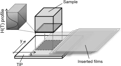
this, a film insertion technique is used as shown in Fig. 2. Electrons escaping from the surface are screened by the in-serted film, depending on their energies. Changing the thick-ness of the inserted film, IP measurements are repeated. Considering all the geometries and the stopping powers of the metal retaining T, the inserted film and IP, the deposited energy in IP given by eq. (3) is calculated with Monte-Carlo simulation program codes. By fitting the calculated results to the experimental ones, the areal T density in depth can be determined. This method has been verified to give the reli-able depth distribution of T concentration in carbon materi-als by Sugiyama et al.17)
3. Experimental
3.1 Samples
The samples used were FCC metals of pure copper (Cu) and pure nickel (Ni), and BCC metals of pure iron (Fe), pure molybdenum (Mo) and pure tungsten (W). Nominal purities of them were above 99.8 mass% except for W which was powder-metallurgical polycrystalline W with the nominal purity of 99.99 mass% (procured from A.L.M.T. Corp.). A
ferritic/martensitic stainless steel (F82H) was also examined
for a future application as first wall of fusion devices. The chemical compositions of the F82H steel were described
elsewhere18); main elements are 8 mass%Cr, 2 mass%W and
balanced Fe. Details of a shape and a size of the sample were described in the following section.
3.2 Hydrogen and tritium loading
H(T) was loaded to the samples either by a gas absorption method or by a glow discharge method. Initial H(T) distribu-tions were set to be homogeneous for the gas absorption, while only surface loaded for the glow discharge.
The gas absorption method with H2 gas of 13.3 kPa and at
873 K for 1 h was conducted for sample sheets of Cu, Ni, Fe
and Mo (10 mm × 10 mm × 0.1 mm) to establish
homoge-neous H(T) distribution in the whole sample volume. The H2
gas contained T with T/H = 1.2 × 10⁻⁶. To observe a depth
profile in near surface region of Cu by the film insertion method, another H(T) loading was conducted with a higher T concentration of T/H = 1.4 × 10⁻⁴.
In order to observe diffusion process in metals, H(T) sur-face loading with a glow discharge method was conducted at
one edge surface of a rod-shaped sample. A cube (6 × 6 ×
6 mm3) of F82H and a disk (ϕ 25.6 mm × 3 mm in
thick-ness) of pure W were exposed to a direct current glow dis-charged (DCGD) plasma in a limited area at one of their
side surfaces through a hole (ϕ 5 mm) of molybdenum mask
as schematically shown in Fig. 3. The temperature of the sample was kept constant during DCGD between 298 K to 674 K. DCGD was carried out with 400 V in voltage under H(T) gas pressure of 62 Pa (T/H = 1.4 × 10⁻⁴). After the
loading, the sample was cooled down to RT with a rate of
about 1 K s−1 by water-quenching of the outside of the
dis-charge vessel to inhibit H diffusion after the loading.
3.3 Surface and depth profiling of T retained in metals
The IP measurements of the loaded surfaces of the Cu, Ni, Fe and Mo samples were conducted for 1 h or 2 h at RT in a light-tight container to obtain surface T profiles. Depth pro-filing of T near the surface region was conducted for the Cu sample by the film-insertion method described in Sec. 2.
After the surface profiling of T, the sample was bisected perpendicular to the H(T) loaded surface using a dia-mond-wire saw in a ventilated glove box and finished within a few hours at RT. The T profiles of the cross-sectional sur-face of F82H and W were determined by the IP
measure-ment for 24 h at a temperature of liquid N2 or below 273 K
in a refrigerator. During the IP measurement, all sample
sur-faces were shielded to avoid the T β-electrons getting in
from other surfaces than the measured cross-sectional sur-face. This method to get the T depth distribution is referred as a cross-sectioning method, hereafter.
Fig. 2 Schematic of depth profiling of T by the film insertion method with
[image:3.595.325.528.620.771.2] [image:3.595.62.274.645.761.2]4. Results
4.1 Surface T distribution of pure Cu, Ni, Fe and Mo
In Fig. 4(a), surface photographs and T profiles for all samples are compared in the same geometrical scale. In the T profiles, relative T intensity is higher as their colors change from blue, yellow and green to red. One can see that the T profiles are quite inhomogeneous with localized high intensity area appeared as small spots all over the surfaces and lines near the edges of the samples. T intensities were averaged over the whole sample surface area and compared with H concentrations calculated with using the reported H
solubility of respective metals19–21) under the present H
loading condition in Fig. 4(b). There is no correlation be-tween the T intensities and the H concentrations at all. The T intensity of Cu was highest, while its H solubility the small-est, i.e. one tens less than that of Ni. This indicates that T observed by TIPT is decoupled from T dissolved in bulk, in other words, most of T observed on the Cu surface is very
likely localized at its surface and/or subsurface but not in
the bulk.
Figure 5(a) shows T depth distribution within a detectable depth of the sample determined by the film insertion method. In the figure, the T intensity averaged over the whole surface area are plotted against the thickness of the inserted film for eight different thicknesses. The insets in the figure are observed surface T profiles for four different thicknesses.Employing reported values of the stopping pow-ers of electrons in Cu and the inserted films, the deposited
energy in IP for the T β-electrons emitted in Cu and passed
through the inserted films were calculated by a Monte-Carlo simulation code (PHITS 2.64, Japan Atomic Energy
Agency22)). In the calculation, compositions of the materials
are chosen as (-(C6H5)-S-) for the inserted film, BaFBr for
the phosphor in IP and pure Cu, and their densities were
1.35, 4.51 and 8.94 g cm−3, respectively. The thickness of
the phosphor in IP was 50 μm. The energy profile of the T
β-electrons was given in the literature23). The cut-off energy
employed in the calculation was 1 keV. In Fig. 5(a), depos-ited energies in IP thus calculated were given for two ex-treme cases, (1) T is fully localized at the top surface given as a dashed line, (2) T is uniformly distributed in Cu given as a dotted line (see also Fig. 5(b)). As clearly seen in the figure, the observed data are between the two but closer to the latter case (the dotted line) than the former case (the dashed line). This indicates depletion of T in the shallower region from the uniform distribution (except the top surface) in the actual T depth profile.
As described in Sec. 2, the deposited energy plotted against the inserted film thickness can be deconvoluted to a T depth distribution. Black dots and line (3) in Fig. 5(b)
show the T depth distribution within 1 μm thus determined.
Lines (1) and (2) in the figure correspond to the two extreme cases in the depth profile discussed above. The T depth pro-file thus obtained is convoluted into the T intensity propro-file against the thickness of the inserted films. The result is given as the solid line in Fig. 5(a) and reproduces the experimental data quite well. The T depth distribution in Fig. 5(b) indi-cates that T was highly localized near the top surface, sig-nificantly depressed within 0.6 μm, and restored a little to a
homogeneous level in the deeper region. Because of the
lim-ited range of the T β-electrons, the T distribution beyond
1 μm in depth could not be determined. Nevertheless, the
decaying distribution from the deep inside to the top surface is quite natural, suggesting diffusive release of homoge-neously dissolved hydrogen in the bulk. The surface local-ized component should be separated from the diffusional component. The cause could be attributed to surface
adsorp-tion of some molecules including hydrogen like H2O, or
trapping at surface defects and/or impurities like surface
oxides.
4.2 Depth distribution of T with a concentration gradi-ent in bulk of F82H and W
It is generally quite difficult to determine H depth distri-butions in endothermic H occluders, because their H solubil-ity is quite small. As noted above, however, quite high sensi-tivity and wider dynamic range in detection of T by TIPT compared to other H detection methods allow depth profil-ing of T in them. In the followprofil-ing, we have observed T depth distribution by the cross-sectioning method to investigate H behaviors in F82H12,13) and pure W11).
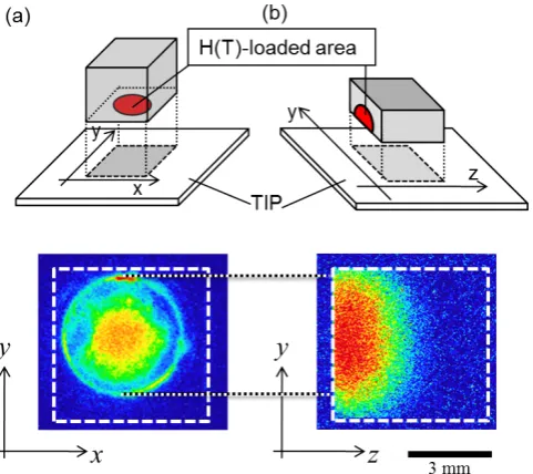
Figures 6 (a) and (b) respectively show T profiles of as-loaded surface and the cross-sectional surface together with schematics of TIPT procedures (Sec. 3.3). The T intensity of the as loaded surface shows two levels with higher density in the central area, while that on the cross-section (Fig. 7(b)) gradual change. The cause of the two levels profile of the as loaded surface is attributed to T trapping at deposited mate-rials (impurities) on a central area owing to a hollow profile in a DCGD column which cause deposition at the central
area, while erosion at surrounding area24). Figure 6 (b)
clearly shows that T diffused into bulk from the loaded sur-face to all other sursur-faces of the cube.
Figure 7 shows a T depth distribution along the central axis of the F82H cube just after the loading for 1 h at 573 K. The T intensity was highest at around 0.8 mm in depth with-out showing the surface accumulation as observed in Cu (Fig. 5(b)). The surface peak caused by surface absorption
and/or trapping was hindered by quite high hydrogen
con-centration in F82H loaded by the plasma discharge. Accordingly the depth distribution decayed towards both di-rections of the loaded surface and the other side surface. The cause of the decay is attributed to diffusional release of T owing to larger hydrogen diffusion coefficients in F82H. Determination of hydrogen diffusion coefficients form the depth distribution in F82H is described later.
5. Discussion
5.1 Determination of hydrogen diffusion coefficients from depth distributions in the endothermic H occluders
It should be noted that TIPT gives profiles of T diluted in H but not pure H nor T. Nevertheless, the T profile reflects the H profile within errors caused by mass difference of H and T, i.e. isotopic effects. In a following section, we have used the term of depth distribution of H concentration (sim-ply as H depth distribution) instead of depth distribution of concentration of T diluted in H and diffusion coefficients of H instead of diffusion coefficient of T diluted in H and discussed H behavior instead of behavior of T diluted in H, allowing errors caused by the isotopic effects (∼√3 ). That is
Fig. 4 (a) Surface photographs and T profiles determined by TIPT for pure Cu, Ni, Fe and Mo after the T loading with using H2 gas including T (T/H = 1.2 × 10⁻⁶) at 13.3 kPa, 873 K for 1 h. (b) Averaged T intensi-ties obtained from T profiles in Fig. 2 and equilibrium H concentration given by H solubility of respective metals under H2 gas at 13.3 kPa and 873 K.
Fig. 5 (a) Dependence of T intensity determined by TIPT on inserted film thickness for a Cu sample with T loaded by the gas absorption method at 873 K for 5 h. Insets are surface T profiles obtained with insertion of four different thickness films. Dashed line (1), dotted line (2) and solid line (3) are theoretical relations corresponding to depth profiles given in (b), (b) Depth profiles; (1) T localized at the surface, (2) T dissolved ho-mogenously in whole thickness, and (3) T profile determined by decon-volution of eq. (3) showing the best fit to the observed dependence (See text).
Fig. 6 Areal distributions of T loaded at 373 K for 3 h to F82H steel by DCGD plasma on (a) the loaded surface and (b) the cross-sectional surface.
[image:5.595.308.549.69.283.2] [image:5.595.47.293.69.202.2] [image:5.595.57.282.294.666.2] [image:5.595.322.530.343.525.2]because temperature dependence of diffusion coefficients of H in most metals usually includes large errors caused by data scattering, and accordingly the errors coming from the isotopic effects are mostly within the experimental errors of the present work. In this section, H diffusion coefficients in F82H and W were determined from the T depth distributions and the validity of the obtained data was discussed in com-parison with the literature data.
H concentration at the loaded surface was constant during the loading since an H influx from plasma and a release flux from the loaded surface were balanced in a steady-state con-dition. Therefore, we selected surface concentration constant as the boundary condition in following diffusion analysis of H loaded by plasma discharge.
Since T diffuses three dimensionally (3d) as appeared in Fig. 6 (b), one dimensional (1d) analysis from the cross-sec-tional surface could have certain error. Therefore,
verifica-tion of the 1d diffusion analysis for a cube (10 × 10 ×
10 mm3) with H loaded by discharge was made. Assuming
that H concentration is zero at all cube surfaces except for the loaded one where the H concentration is kept constant during the loading, H concentration in the cube, c(x, y, z), was determined by numerically solving 3d Fick s diffusion equation using H diffusion coefficient of 1 × 10⁻¹¹ m2 s−1
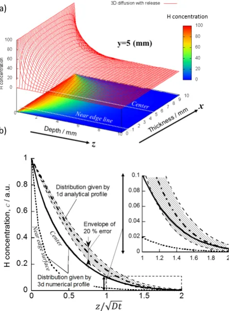
for a diffusion time of 2 h at 473 K as in the case for pure W. Figure 9(a) shows a profile of the H concentrations on the
central plane of the cube, c(x, 5, z), as contours and planer projection with colors changing from red, yellow, green and blue corresponding to higher to lower concentrations. The figure clearly shows concentration decays towards all side surfaces, indicating diffusional release from the all surfaces. The H depth distributions along the central axis, x = 5, and a near edge line, x = 0.5 indicated in Fig. 9(a) are shown in Fig. 9(b) in which z axis is converted to the normalized dif-fusion length (z/√Dt ). In the figure, an analytical solution of 1d Fick s equation given below is also plotted for comparison,
c(z)=c0er f c z
2√Dt , (4)
where c0 is the constant H concentration at the loaded
sur-face during the loading and D is an H diffusion coefficient. Although the 1d analytical solution deviates from the 3d nu-merical solution in shallower region, the former becomes closer to the latter in deeper region and the latter lies within the envelope of 20% errors of the former as depicted in the enlarged inset of Fig. 9(b). In deeper region, or with increas-ing the depth (thickness perpendicular to the loaded surface) the error becomes less. Considering the geometry of the present samples, the values of D determined with the 1d analysis given below have errors less than 20% error. Note that release of H after the loading and during a cooling could
Fig. 8 T depth distributions in pure W just after the loading by plasma dis-charge at (a) 473 K and (b) 773 K for 2 h. Insets are enlarged in vertical axis and shortened in horizontal axis to make the depth distribution near surface clearer. Diffusion coefficients given in the figures are determined by data fitting (see text).
[image:6.595.52.287.69.400.2] [image:6.595.310.546.70.390.2]also change H depth distributions, which is discussed in sec-tions of 5.1.1 and 5.2.
5.1.1 H diffusion coefficients in F82H
Although H diffusion coefficients determined by the 1d diffusion analysis of the T depth distribution obtained from the cross-sectioning method include some errors as dis-cussed above, the analysis using the T depth distribution limited for deeper region reduces the error. In the following, H diffusion coefficients are determined from the 1d analysis of the T depth distributions obtained by TIPT for more than 1 mm deeper region. Accordingly, the error would be much less than 20% as depicted in Fig. 9(b).
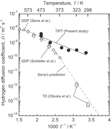
Figure 10 shows thus determined H diffusion coefficients from the T depth distributions given in Fig. 7 for F82H. The figure also contains some literature data determined by a
gas-driven permeation (GDP) by Serra21) and Schliefer25)
and a tritium desorption by Otsuka26). The latter two
appre-ciably deviate downward from the extrapolation of the Serra s data in lower temperature range, while the present data are just on the extrapolation. This indicates that the present data are most likely corresponding to interstitial dif-fusion of H dissolved in F82H within 20% of uncertainty.
As noted in Fig. 7, the experimental H depth distribution near surface region appreciably deviates from the analytical solution (eq. (4)) given as a dashed line. This is most likely caused by H release from the loaded surface during the cool-ing (around 1 minute) after termination of the loadcool-ing. Assuming that H was released by diffusion for 1 min at the loading temperature just after termination of the loading, a depth distribution was numerically calculated by the 1d dif-fusion analysis resulting in solid line in Fig. 7. Although the near surface concentration in the calculated distribution is less than the observed one, the maximum H concentration at the depth of 1 mm and the distribution in the 1–3 mm range represent well the observed one. The distribution in the deeper region was not subjected to change by the surface re-lease, so as the diffusion coefficients determined from the depth distribution in the deeper region.
The appearance of excess H (remaining H) near surface region can be attributed to H trapped in the near surface
re-gion or H2O adsorbed at the surface, suggesting that the data
deviating downwards in Fig. 10 are influenced by the surface H in determination of their diffusion coefficients. Because of its endothermic nature, dissolved H in F82H should decrease exponentially with decreasing temperature, while the surface localized H stays rather constant. Hence, the deviation of the apparent diffusion coefficients become more appreciable at lower temperatures.
5.1.2 H diffusion coefficients in pure W
H diffusion coefficients in W are also determined with us-ing the same 1d diffusion analysis as F82H from the T depth distributions beyond 0.5 mm in depth. In Figs. 8 (a) and (b) are plotted the 1d analytical solutions showing the best fit to reproduce the observed distributions. Figure 11 shows tem-perature dependence of H diffusion coefficients in pure W thus determined. In the figure, literature data determined by
GDP by Frauenfelder27) and Zakhalov28), an ion-driven
per-meation (IDP) by Nakamura29), Lee30) and Gasparyan31), and
a thermal desorption spectroscopy (TDS) by Esteban32) and
Franzen33) including our previous studies using TIPT11), are
also given for comparison. The data obtained by TIPT agree quite well with the extrapolated values of the Frauenfelder s data obtained above 1173 K to the present temperature range. Including the Frauenfelder s data, the Ikeda s data and the present data, a reliable set of diffusion coefficients of H interstitially dissolved in W is given by
D=(3.8±0.4×10⁻⁷)exp −0.39±0.03[eV]
kBT , (5)
where kB is the Boltzman constant in eV·K−1, and T is tem-perature in K.
[image:7.595.312.540.516.733.2]As seen in Figs. 8 (a) and (b), significantly large amount of H was retained in near surface regions at both the loaded
Fig. 10 Temperature dependence of H diffusion coefficients in the F82H steel. Literature data determined by GDP by Serra21) and Schliefer25) and a tritium desorption by Otsuka26) are also given for comparison.
[image:7.595.79.261.544.753.2]surface and the opposite (back) surface compared to the amount of H retained in the deeper region. Assuming the de-cay of the near surface-localized component was also caused by diffusion, another set of diffusion data, D ∗ and D ∗∗, were
determined and plotted in Fig. 11. These diffusion data for the surface-localized components are roughly two orders of magnitude smaller than that for the interstitial diffusion (D). In addition, their temperature dependence is quite weak. Therefore, we can conclude that the surface-localized com-ponent is strongly trapped.
It is important to note that the apparent diffusion coeffi-cients determined from the surface-localized component are close to most of the literature data. Furthermore, the amount of H retained in the near surface region was much larger than that in the deeper region by orders of magnitude. If dif-fusion coefficients were determined by observation of H lease, the values would correspond to the release of H re-tained in the near surface region, but not to H dissolved interstitially in the bulk. This suggests that most of the diffu-sion coefficients in previous works determined by release behaviors of H are not likely correspond to the bulk diffu-sion coefficients.
[image:8.595.48.290.439.705.2]5.2 Release behaviors of H retained at surface, and in subsurface and bulk of metals
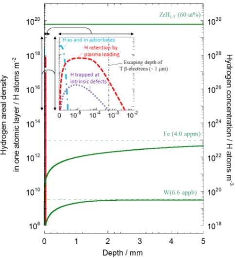
Figure 12 compares calculated H depth distributions within 5 mm from the surface for Zr, Fe and W with the loading by gas absorption at 13.3 kPa and 573 K up to their solubility limits and followed H release afterwards for
10 min at the same temperature. The calculation was made assuming diffusion controlled dissolution and release with diffusion coefficients expected form extrapolation of the re-liable literature data obtained at higher temperatures27,34) to
573 K.
Owing to exothermic nature, H is not released from Zr keeping the original uniform distribution of zirconium
hy-dride (ZrH1.5), while in Fe and W, the endothermic H
oc-cluding metals, appreciable amount of H once dissolved is released by diffusion showing the distribution decay from the deep inside to the surface. Actually, the decaying distri-butions in the deeper region of Fe and W obtained by TIPT agree well with the calculated H distributions to give reliable bulk diffusion coefficients.
At surface and in subsrface, depth distributions deter-mined by TIPT, particularly for the endothermic occluders appreciably deviate from those of dissolved H, as shown in the inset of Fig. 12. Within a few atomic layers of the sur-face including the top sursur-face to a few nm in depth, there
al-ways exist adsorbed H atoms and/or H included in
adsor-bates such as ubiquitous water molecules (distribution given by a dashed and dotted line). Furthermore there could be chemically modified layers by impurities included in metals as often appearing as surface precipitates like oxide, carbide, nitride and some others, which also absorb H. Beneath such the surface layers, H is rather densely trapped in various de-fects introduced by surface preparation such as cutting, grinding and polishing and also in the oxide layers (distribu-tion given by a dotted line).
In case of plasma loading, there appears plasma-induced H saturated layers not only within a projection range of
im-pinged ions or atoms but also spreading into 10 μm in depth
owing to excess loading of H from plasma11) (distribution
given by a dashed line).
The significant H retention in the surface and subsurface is appreciable mainly in endothermic H occluders as de-picted in the figure. H is chemically bound in the layers and hardly released at the loaded temperature. Integrated amount
of H retained in the surface layers within a few μm is likely
much larger than that of the dissolved H. Accordingly, diffu-sion coefficients determined by thermal desorption of the whole retained H or depth distributions in near surface re-gions could underestimate diffusion coefficients compared with those determined from H dissolved in bulk.
6. Conclusions
We have established TIPT as a new tool to observe depth distributions of H in metals with the cross-sectioning method. Owing to its very wide dynamic range for detection of T by TIPT, 4–5 digits, it gives quite detailed depth distri-butions of H in a metals from its top surface to deep inside (over cm range). Such detailed depth distribution allows us to separate H diffusive species from trapped ones and to de-termine reliable diffusion coefficients in metals having very low H solubility like F82H and W.
The depth distributions are quite different depending on heat of solution of H in metals, i.e. (1) endothermic or (2) exothermic: (1) High H concentration in exothermic H oc-cluding metals hinders surface localized H. Correspondingly
the H depth distributions determined by the cross-sectioning method with TIPT well represents distributions of H dis-solved or chemically bound to metal atoms (forming hy-drides) in bulk. (2) In endothermic H occluding metals, the H depth distributions determined by the cross-sectioning method shows surface localization of H with quite tiny H dissolved in bulk. Because of endothermic nature with large H diffusion coefficients, H once occluded in the metals is desorbed via H diffusion in near surface regions. Accordingly, H remained in near surface region is limited to trapped ones or H with other different chemical forms. Moreover, owing to their low solubility, the amount of H or concentration of H in their bulk is quite small and only TIPT allows to observe. Although such near surface profiles of H can be obtained by ion beam analyses, their behavior does not correspond to that of H dissolved in bulk. Accordingly, apparent diffusion coefficients determined from the near
sur-face profiles and/or their desorption might be different from
bulk diffusion coefficients.
Acknowledgement
This work was supported by Grant-in-Aid for Scientific Research on Priority Area 467 Tritium for Fusion The Ministry of Education, Culture, Sports, Science and Technology (MEXT) No. 190550088, 20049006 and 22017005.
REFERENCES
1) J. Völkl and G. Alefeld: Diffusion of hydrogen in metals, (Springer-Verlag, Berlin Heidelberg New York, 1978) pp. 321–348.
2) R.A. Causey: J. Nucl. Mater. 300 (2002) 91–117.
3) T. Tanabe, Y. Yamanishi and S. Imoto: J. Jpn. Inst. Metals 25 (1984) 1–10.
4) K. Hashizume, M. Sugisaki, K. Hatano, T. Ohmori and K. Ogi: J. Nucl. Sci. Technol. 31 (1994) 1294–1300.
5) K. Fujii, K. Hashizume, Y. Hatano and M. Sugisaki: J. Alloy. Compd.
270 (1998) 42–46.
6) H. Saitoh, T. Misawa, Y. Noya and T. Ohnishi: Mater. Trans., JIM 40 (1999) 692–695.
7) H. Saitoh, H. Homma, T. Misawa and T. Ohnishi: Mater. Trans. 42 (2001) 399–402.
8) T. Hirano, Y. Saruwatari, K. Hashizume, T. Otsuka and T. Tanabe: Proc. E-MRS IUMRS ICEM 2006 (2006).
9) K. Hashizume, J. Masuda, T. Otsuka, T. Tanabe, Y. Hatano, Y. Nakamura, T. Nagasaka and T. Muroga: J. Nucl. Mater. 367–370 (2007) 876–881.
10) K. Hashizume, K. Ogushi, T. Otsuka and T. Tanabe: J. Nucl. Mater.
417 (2011) 1175–1178.
11) T. Otsuka, T. Hoshihira and T. Tanabe: Phys. Scr. T138 (2009) 014052.
12) T. Otsuka and T. Tanabe: J. Alloy. Compd. 580 (2013) S44–S46. 13) M. Higaki, T. Otsuka, K. Tokunaga, K. Hashizume, K. Ezato, S.
Suzuki, M. Enoeda and M. Akiba: Fus. Sci. Technol. 67 (2015) 379–381.
14) Y. Iwabuchi, N. Mori, K. Takahashi, T. Matsuda and S. Shionoya: Jpn. J. Appl. Phys. 33 (1994) 178–185.
15) H. Ohuchi-Yoshida, Y. Hatano, Y. Kino and Y. Kondo: Fusion Eng. Des. 87 (2012) 423–426.
16) M. Matsuyama, T. Murai and K. Watanabe: Fus. Sci. Technol. 41 (2002) 505–509.
17) K. Sugiyama, T. Tanabe, K. Miyasaka, K. Masaki, K. Tobita, N. Miya, V. Philipps, M. Rubel, C.H. Skinner, C.A. Gentile, T. Saze and K. Nishizawa: J. Nucl. Mater. 329–333 (2004) 874–879.
18) M. Tamura, H. Hayakawa, M. Tanimura, A. Hishinuma and T. Kondo: J. Nucl. Mater. 141–143 (1986) 1067.
19) W.M. Robertson: Z. Metallk. 64 (1973) 436–443.
20) T. Tanabe, K. Sawada and S. Imoto: T. Jpn. I. Met. 27 (1986) 321–327.
21) E. Serra, G. Benamati and O.V. Ogorodnikova: J. Nucl. Mater. 255 (1998) 105–115.
22) T. Sato, K. Niita, N. Matsuda, et al.: J. Nucl. Sci. Technol. 50 (2013) 913–923.
23) P. C. Souers: Hydrogen properties for fusion energy, (University of California Press, Berkley and Los Angels, 1984) pp. 1–14.
24) T. Otsuka, M. Shimada, T. Tanabe and J.P. Sharpe: Fus. Sci. Technol.
60 (2011) 1539–1542.
25) F. Schliefer, C. Liu and P. Jung: J. Nucl. Mater. 283–287 (2000) 540–544.
26) T. Otsuka and T. Tanabe: Fus. Sci. Technol. 54 (2008) 541–544. 27) R. Frauenfelder: J. Vac. Sci. Technol. 6 (1969) 388–397.
28) A.P. Zakharov, V.M. Sharapov and E.I. Evko: Fiz. Khim. Mekh. Mater. 9 (1973) 29–33.
29) H. Nakamura, W. Shu, T. Hayashi and M. Nishi: J. Nucl. Mater. 313–
316 (2003) 679–684.
30) H.T. Lee, E. Markina, Y. Otsuka and Y. Ueda: Phys. Scri. T145 (2011) 014045.
31) Y.M. Gasparyan, A.V. Golubeva, M. Mayer, A.A. Pisarev and J. Roth: J. Nucl. Mater. 390–391 (2009) 606–609.
32) G.A. Esteban, A. Perujo, L.A. Sedano and K. Douglas: J. Nucl. Mater.
295 (2001) 49–56.
33) P. Franzen, C. Garcia-Rosales, H. Plank and V.K. Alimov: J. Nucl. Mater. 241–243 (1997) 1082.