A Three Dimensional Cellular Automaton Model for the Prediction of Solidification Morphologies of Brass Alloy by Horizontal Continuous Casting and Its Experimental Verification

The purpose of this study is to predict the morphologies of the solidification process for brass alloys (Cu70Zn30 and Cu65Zn35) by horizontal continuous casting (HCC) and to verify its accuracy by the observed experimental results. This study was extended from previous study (predict the solidification microstructure of pure copper rod by vertical continuous casting process). In numerical simulation aspect, finite difference method (FDM) and cellular automaton (CA) model were utilized to solve the macro-temperature field and micro-nucleation and grain growth of brass alloy respectively. From the observed casting experiment, the unidirectionally solidified brass rod could be fabricated by the HCC process with using cooled mold. The cast grain morphology by CAFD model was corresponding to the result of actual casting experiment well. [doi:10.2320/matertrans.M2010402]

(Received November 30, 2010; Accepted January 21, 2011; Published April 1, 2011)

Keywords: brass alloy, horizontal continuous casting, solidification microstructure, cellular automaton model, finite difference method

1. Introduction

Brass has higher malleability than copper or zinc. The relatively low melting point of brass and its flow character-istics make it a relatively easy material to cast. By varying the proportions of copper and zinc, the properties of the brass can be changed, allowing hard and soft brasses. Horizontal Continuous Casting (HCC) is one of the main methods used to produce brass rods. After further mechanical processing, such as drawing, wires and tubes with high purity and homogeneity can be directly applied to various devices. Brass has many advantages via HCC, such as the direct cold rolling processing, less equipment investment and environmental pollution, shorter period of construction cycle and technical process, quick, effective, energy conservation, flexibly producing, high rate of finished products, the lower produc-tion cost, the better economic efficiency, etc. The malle-ability and acoustic properties of brass have made it the metal of choice for brass musical instruments.

Solidification, the most important process in HCC, deter-mines the formation of the bulk microstructure, which is directly related to the mechanical and chemical properties. In the HCC process, various casting conditions such as casting speed are manipulated, which in turn affects the temperature gradient and growth rate, to control the microstructure formation during solidification and thus serves to improve the specified properties. Earlier studies were conducted on the basis of physical observation and metallurgical analysis on actual casts under various operating conditions. Although viable, these methods involve a lot of manpower, resources, and time. It is thus desirable to utilize numerical modeling techniques to simulate the solidification microstructure. Using numerical simulation, predictions can be made for microstructural changes with respect to casting conditions.

Two major methods can be used to model cast micro-structure, deterministic and probabilistic. The deterministic

method is based on the kinetics of solid-state transformation during solidification, with nuclei density and growth rate considered as a function of undercooling. In 1966, Oldfield associated heat transfer with grain growth to simulate the crystallization of grey iron, in which nucleation changes constantly in proportion to the square of undercooling.1)In 1984, Hunt published a model for instantaneous nucleation in continuation with applying the deterministic methods.2) In terms of categorizing the crystals formed, Dunstin and Kurz assumed the growth of spherical, columnar, and cylindrical equiaxed grains.3)_{Their revised method focused on} simulat-ing the number of grains and average grain size in several zones of interest. Although the deterministic method is derived from solidification kinetics and physically satisfies conditions for grain growth, it fails to consider heat flow and the general randomness of the nucleation process.

More recently, emphasis has been put on integrating the advantages of the two models. Rappaz and Gandin developed a Cellular Automation (CA) method based on the heteroge-neous nucleation and the continuous nucleation models.4–7) The continuous nucleation model integrates the Gaussian distribution between nucleation densities and undercooling. In the CA model, nucleation locations and preferential growth orientation are determined using the probabilistic model; whereas the growth rate of dendrite tips is modeled with the deterministic model based on physics theories.

developed a CA method that can simulate microstructure evolution during eutectic and peritectic solidification.11) Some modified CA models that directly solve the transport equations at the solid-liquid interface have been developed to simulate dendritic growth patterns.12)_{Further developments} of the CA model are coupling the phase-field method (PF-CA model) for the simulation of formation of macrostructures in multi-component alloy systems.13) _{The effect of} macro-segregation also has been developed to account for structure formation compared to purely macroscopic models.14)

In the present study, a microstructure prediction system for the HCC process based on the Cellular Automaton (CA) model is developed. The system is then tested by comparing the actual cast observations with simulation results on microstructural changes of brass alloys.

2. Experimental Method

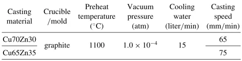
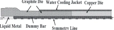
The proposed study adopted the HCC process to fabricate brass rods. In the HCC process, a vacuum furnace and continuous casting techniques are used to develop products with a high level of cleanliness and purity. The HCC device is shown in Fig. 1, and the experimental parameters used in this study are shown in Table 1. Graphite moulds made of carbon IG15 and copper mould were used for the HCC process. As shown in Fig. 2, one graphite mould was 2 cm in diameter and 12 cm in height, the other was 2 cm in diameter and 10 cm in height and the copper mould was 2 cm in diameter and 17 cm in height. A typical experimental procedure began with the vacuum smelting of pure copper and zinc metals at a pressure of 1:0104atm and the carbon crucible being preheated to 1100C. The drawing was conducted at a constant casting speed with a cooling water flow rate of 15 L/min, resulting in a brass rod with a diameter of 6 mm. The

temperature profiles at various locations were measured and recorded throughout the experiment. As shown in Fig. 3, the point #1 was set to gain the temperature when the procedure reached stable. The casting was cut into multiple sections and embedded in epoxy-based modules. Grinding, polishing, and etching with HNO3 + H2O (1 : 1) were then performed (etching time of 17 s). An optical microscope was used to observe the microstructures of the brass rod fabricated under various casting conditions.

Fig. 1 Schematic illustration of the casting equipment of HCC.

Table 1 Experimental parameters of HCC process.

Casting material

Crucible /mold

Preheat temperature

(_C)

Vacuum pressure (atm)

Cooling water (liter/min)

Casting speed (mm/min) Cu70Zn30

graphite 1100 1:0104 ₁₅ 65

Cu65Zn35 75

(a)

(b)

Fig. 2 Photograph of mould used in HCC process (a) graphite mould (b) copper mould.

simulation in this study is shown in Fig. 4. The symmetry of cylinder is considered. Liquid metal is shown at the centre and a dummy bar with the diameter of 6 mm is used to continuously draw a brass rod through the graphite mould in a vacuum, with water cooling surrounding the model. The related numerical simulation methods are described below.

3.1 Heat flow calculation in HCC process

In the present simulation, the finite difference method was used to calculate transient heat transfer in the HCC process. The governing equation is given by

Cp

@T @t ¼

@2_T

@r2 þ

1

r @T @r þ

@2_T

@z2

Cpvc

@T

@zþqq_ ð1Þ

whererandzare the grid size with the length of 0.5 mm,is the density, Cp is the specific heat, is the thermal conductivity,vcis the casting speed, andqq_is the latent heat obtained using the modified temperature recovery method.15) The boundary conditions at the melt/mould interface and the mould/water interface are given by:

Melt/mould:

q¼hintðTmouldTmeltÞ ð2Þ

Mould/water:

q¼hwðTwaterTmouldÞ ð3Þ

where q is the heat flux, Tmelt, Tmould and Twater are the temperatures of the melt, the mould, and the cooling water, respectively, and hint and hw are the interfacial heat coefficients at the melt/mould and the mould/water inter-faces, respectively. The governing equation and boundary condition for heat transfer shown in eqs. (1), (2), and (3) are solved using an explicit difference algorithm.

3.2 Nucleation and growth algorithm

Nucleation is the dominant stage of microstructural evolution in solidification, which leads to the establishment of the final grain population. From previously mentioned theories, a heterogeneous nucleation model is adopted to explain the nuclei density increasedninduced by an increase in the undercooling dðTÞ according to the following Gaussian distribution:

dn

dðTÞ¼ nmax

ffiffiffiffiffiffi 2 p

ðTÞexp

1 2

TTN

T

2

" #

ð4Þ

The Gaussian distribution is determined by three parameters:

nmax: maximum density of nuclei given by the integral of the Gaussian distribution from01

other two relationships to the undercooling. Finally, we can gain the simultaneous equations and solve them to obtain the nucleation parameters.

Thus, the density of grain nðTÞ formed at a certain undercoolingT is given by:

nðTÞ ¼

ZT

0

dn

dðTÞdðTÞ ð5Þ

Certain CA cells would start nucleation when sufficient undercooling is provided. During any time-step, t, the temperature of the specimen decreases by an amount,T, and thus the undercooling increases by an amount, ðTÞ. The density of new grains which are nucleated within the volume of melt is given by

n¼n½TþðTÞ nðTÞ ¼

ZTþðTÞ

T

dn

dðTÞdðTÞ

ð6Þ

Meanwhile, new grain would lead to the increase in grain density, randomly distributed inside the CA cell. n is then multiplied by the total volume of the specimen to give the number of grains, N, which is divided by the number of cells, NCA to give the probability of nucleation, Pn, where

VCA is the volume of cell. During each time step, cells defining the volume of the specimen are scanned and a random number is givento each one of them (055_1).

CA cells transform from liquid to solid when5_Pn.

Pn¼

N

NCA

¼nVCA ð7Þ

Pn: Probability of nucleation

N: Number of newly formed nuclei

NCA: Total number of cells

VCA: The volume of an individual cell

n: The increase of grain density

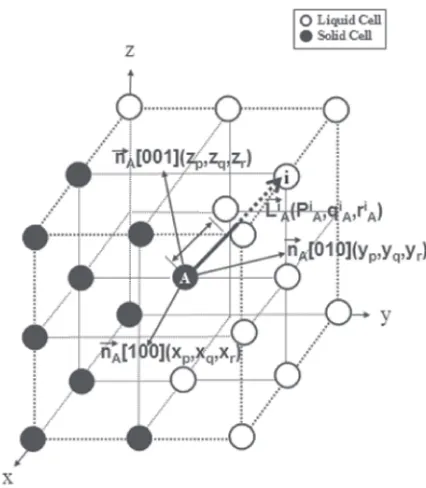
Once a cell has nucleated, it grows with a preferential direction corresponding to its crystallographic orientation. An algorithm for grain growth with various preferred orientations constructed using three Euler angles was embedded into the CA growth algorithm by Hong.16,17)_The algorithm randomly reproduces the preferentialh100igrowth direction of FCC or BCC metals. Thus, during a time step interval used for integrating the growth kinetics of the dendrite tips, the growth length of the solidified cell v with respect to its liquid neighbor cell i (as shown in Fig. 5) is

Li_vðtÞ, which can be calculated using:

Li_vðtÞ ¼W_viX N

n¼1

where t is the time step, Wi

v is the orientation weight coefficient, and N is the iteration number. The orientation weight coefficientW_vi is given by:

W_vi ¼Max½jXwj;jYwj;jZwj ð9Þ

whereXw,YwandZwcan be calculated using

Xw

Yw

Zw

2 6 4

3 7 5¼

xpxqxr

ypyqyr

zpzqzr

2 6 4

3 7 5

pi v

qi v

ri v

2 6 4

3 7

5 ð10Þ

whereðxp;xq;xrÞ,ðyp;yq;yrÞ andðzp;zq;zrÞare the direction cosines of the [100], [010], and [001] dendrite arms related to the coordinate x,y, andzaxes, respectively. ðpi

v;qiv;rviÞare the direction cosines of the vector LL~i

v, related to the coordinatex,y, andzaxes, respectively. For a more detailed description of the growth algorithm, refer to Ref. 15). The growth kinetics of both columnar and equiaxed grains can be calculated with the aid of the Kurz-Giovanola-Trivedi (KGT) model.18)The dendrite tip radius,R, and growth velocity,v, are determined by the two relationships

¼ C

_C 0

C_ð1k 0Þ

¼IvðPeÞ ð11Þ

and

R¼2

ffiffiffiffiffiffiffiffiffiffiffiffiffiffiffiffiffiffiffiffiffiffiffiffiffiffi

ðmGccGÞ

s

ð12Þ

is the solute supersaturation,C_{is the liquid concentration} at the tip,C0 is the initial concentration, k0 is the partition coefficient, is the Gibbs-Thomson coefficient, m is the liquidus slope, Gc is the solute gradient, G is the thermal gradient, Dl is the solute diffusion coefficient in the liquid phase andcis a function of the solute Peclet number, which value is close to unity.IvðPeÞis the Ivantsov function of the solute Peclet number. The solute Peclet number,Pe, is given by

Pe¼ R

2Dl

ð13Þ

Therefore, the relationship between the growth rate of the dendrite tip, v, and its undercooling, T, is given by the solution of eqs. (11)–(13).

vðTÞ ¼ Dl

5:512_ðmð1k 0ÞÞ1:5

T2:5

C1:5 0

ð14Þ

In order to simplify the calculation of growth velocity, the eq. (14) is turned into a polynominal regression expression as a function of the degree of local undercooling, as shown in Figs. 6 and 7.

For the Cu70Zn30:

vðTÞ ¼3:0106T3þ1:0105T2

4:0105Tþ3:0105 ð15Þ

For the Cu65Zn35:

vðTÞ ¼3:0106T3þ8:0106T2

3:0105Tþ2:0105 ð16Þ

Then, the solid fraction of the liquid cell i at a certain time

fi

sðtÞcan be expressed by:

f_siðtÞ ¼L

i vðtÞ

L ð17Þ

whereLis the spacing between the cell v and liquid cell i. When f_siðtÞ=_{1, which means that the growth front of cell v}

can touch the center of the liquid cell i, the liquid cell i transforms its state from liquid to solid and adopts the same orientation index as that of cell v.

Fig. 5 Schematic diagram of the growth algorithm used in the CA model.

Fig. 6 Growth kinetics of a dendrite tip, as calculated using the KGT model for Cu70Zn30. (R2_{is the square of the correlation coefficient)}

3.3 Determination of the time step

In order to reduce the computational time, two time steps were used, one for the macroscopic heat transfer calculation and the other for the microscopic CA calculation.

macro time step:

tT¼

r2_C p

5 ð18Þ

micro time step:

tCA¼

dx

5Vmax

ð19Þ

wheredxis the cell size andVmax is the maximum growth velocity obtained by scanning the growth velocities of all interface liquid cells during each time step.

The flowchart for the microstructure simulation of a brass rod under the HCC process is shown in Fig. 8. The simulation procedure using the coupled macro-micro model are as follows: first, the simulation system is initialized with the domain length, mesh size, and initial temperature; second, the energy equations in the liquid and the solid regions are solved; third, whether a certain liquid cell nucleates or a certain solid cell grows with a certain growth velocity is estimated using the CA model based on the calculated temperature in the CA cells. At this stage, the liberation of latent heat in the solidifying cells is estimated using the temperature recovery method. Finally, using the updated temperature calculation for the new liquid region can be continued. This series of calculations is repeated until the end of solidification. The thermal and physical properties used in the present calculations are listed in Tables 2 and 3. The actual nucleation parameters are important and should be determined by the DTA experiment. However, in this study the most appropriate values to be used for the parameters were obtained from related papers as cited and then verified by the computer simulation results. These appropriate

nucleation parameters were obtained from Ref. 19). The simulated and experimentally observed microstructures were compared to examine the reliability of the proposed simulation technique.

4. Results and Discussion

The examination of the HCC process is described in two parts. In the first part, the actual process of HCC is used to observe changes in the evolution mechanism of solidification microstructure with respect to casting speed. In the second part, the finite difference method is used to calculate the macroscopic temperature fields and the CA method is used to compute microscopic nucleation and growth mechanism; thus, the macro and micro scale effects are coupled on the final microstructure.

4.1 HCC process of brass alloy

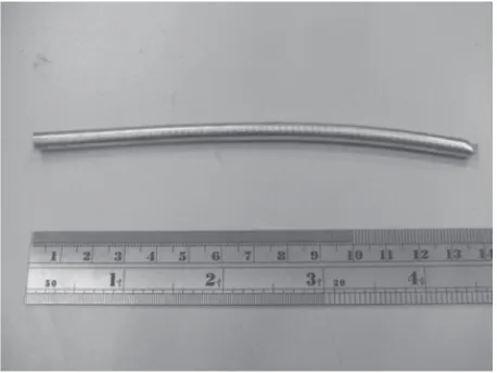
First, using the dummy bar with different casting speeds to draw the brass rod horizontally and then twist the brass rod by the coil device. Figure 9 describes the actual HCC process. Figure 10 displays the finished 6mm diameter brass rod (Cu70Zn30) of 65 mm/min casting speed. The metal surface appeared smooth and flat. The measured temperature of point #1 is between 635 and 639_{C when the casting situation is} stable. In order to examine the versatility of the simulation system in HCC process, taking another case into consider-ation.

4.2 Temperature distribution in HCC process

For the macroscopic purpose of this study, finite difference methods were used to solve the two dimensional heat transfer equations. The resulting temperature distribution is shown in

Fig. 8 Numerical simulation flowchart of microstructure modeling for HCC process.

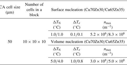
Table 3 Parameters for microstructure modeling of HCC process.

CA cell size (mm)

Number of cells in a

block

Surface nucleation (Cu70Zn30/Cu65Zn35)

TN

(_C)

T

(_C)

nmax

(m2₎

1.0/1.0 0.1/0.1 5:2106_=8:3106

50 101010 Volume nucleation (Cu70Zn30/Cu65Zn35)

TN

(_C)

T

(_C)

nmax

(m3₎

Fig. 11(a), where obvious observations can be made, the heat transfer mechanism is along axial direction. The location of point #2 is equal to the location of point #1 and the temperature of point #2 is 632_{C when the temperature field} reaches the steady state. The temperature result of numerical simulation approaches the temperature of actual HCC process. Figure 12(a) shows that when casting speed is

increased (75 mm/min), the position of the S/L interface moves closer to the exit of the mould. Figures 11(b) and 12(b) describes the solid fraction of brass rod and show the size of mush zone. The mush zone size of the brass rod is narrow, so the effect of microsegregation is not serious in the brass rod. The symmetry in cylindrical coordinates allows the (a)

(b)

Fig. 9 The actual situation of brass rod in HCC process (a) rod-drawing process (b) coil device.

Fig. 10 Withdrawal6mm brass rod (Cu70Zn30) after HCC process.

(b) (a)

Fig. 11 6mm brass rod (Cu70Zn30) for a casting speed of 65 mm/min in HCC process (a) temperature field (b) solid fraction.

(b) (a)

2-D temperature to be expanded to a 3-D temperature in the 3D-CA model to simplify the calculation of the simulation process and to speed up the calculation time. The 3-D macroscopic temperature field is used as the basis for the development of microscopic nucleation and growth models.

4.3 Verification of Brass alloy microstructure simula-tion

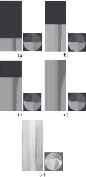
Since a 3-D model requires large storage resources for proper results, it is beneficial to simplify the methodology and combine the results of two dimensional cross sections to create a three dimensional model. Figure 13 shows the microstructure of the6mm brass (Cu70Zn30) rod obtained from casting with a 65 mm/min casting speed and 15 L/min flow rate of cooling water. Figure 13(a), (b), (c) and (d) show the simulation results of the transverse and longitudinal sections, respectively. In the longitudinal section, the grains have a parallel columnar structure and the grain growth follows the axial direction with different time steps. The evolution of grain growth is similar to that predicted from the temperature gradient direction. In the transverse section, the smaller grains are eliminated and the bigger ones are getting thick. Figures 13(e) shows the metallography of the brass (Cu70Zn30) rod. It’s obvious that the grain morphogy is unidirectionally solidified in the longitudinal section and there are only two grains exist in the transverse section. Comparing with the metallography, it could be found that the simulated results were similar to the actual casting.

Figure 14 shows the microstructure of the 8mm brass (Cu65Zn35) rod obtained from casting with a 75 mm/min casting speed and 15 L/min flow rate of cooling water. As shown in Figs. 14(a), (b), (c) and (d), there are some parallel columnar grains keep the axial growth in the longitudinal section and several grains get coarser in the transverse section. Figures 14(e) shows the metallography of the brass (Cu65Zn35) rod. Comparing with Figs. 13(e), it’s obvious that there is a rise in grain number. This result could be attributed to an increase in casting speed and cast size, leading to reduce the effect of grain growth competition.20) The predictions of the solidification microstructures obtained using the proposed numerical simulation system based on a CAFD model are similar to the results of the actual casting experiment.

5. Conclusions

(1) Using the finite difference method to obtain the macro temperature field, then coupling the CA model to calculate the nucleation and grain growth could effectively predict the microstructure morphology of brass alloy by HCC process.

(2) The unidirectionally solidified brass rod could be fabricated by optimization of withdrawal speed during the HCC process using cooled mold.

(c)

(e)

(d)

Fig. 13 Solidification microstructure of6mm brass rod (Cu70Zn30) for a casting speed of 65 mm/min. (a) Simulated microstructure at 378 s, (b) simulated microstructure at 387 s, (c) simulated microstructure at 396 s, (d) simulated microstructure at 399 s, and (e) metallograph of actual cast. (Left: longitudinal section, Right: transverse section)

(c) (d)

(e)

Acknowledgment

The authors would like to thank Wan-Lung Corporation and Technology Development Program for Academia (98-EC-17-A-05-S1-122) in Taiwan for the financial support of this study.

REFERENCES

1) W. Oldfield: ASM Trans.59(1966) 945. 2) J. D. Hunt: Mater. Sci. Eng.65(1984) 75. 3) I. Dustin and W. Kurz: Z. Metallkd.77(1986) 265. 4) C. A. Gandin and M. Rappaz: Acta Mater.42(1994) 2233.

5) C. A. Gandin, J. L. Desbiolles, M. Rappaz and P. Thevoz: Metall. Mater. Trans. A30(1999) 3153.

6) M. Rappaz and C. A. Gandin: Acta Mater.41(1993) 345.

7) M. Rappaz, C. A. Gandin, J. L. Desbiolles and P. Thevoz: Metall. Mater. Trans. A27(1996) 695.

8) Y. Hirokazu and O. Itsuo: J. Japan Inst. Metals61(1997) 342. 9) K. Harkki and J. Miettinen: Metall. Trans. B30(1999) 75. 10) Y. T. Ding and G. J. Xu: Foundry Technology26(2005) 1075. 11) M. F. Zhu and C. P. Hong: Metall. Mater. Trans. A35(2004) 1555. 12) H. B. Dong and P. D. Lee: Acta Mater.53(2005) 659.

13) Y. Natsume and K. Ohsasa: ISIJ Int.46(2006) 896.

14) G. Guillemot, C. A. Gandin and M. Bellet: J. Crystal Growth 303

(2007) 58.

15) X. G. Qu and X. Q. Li: Machin. Design Manuf.1(2008) 109. 16) Y. H. Chang, S. M. Lee, K. Y. Lee and C. P. Hong: ISIJ Int.38(1998)

63.

17) M. F. Zhu and C. P. Hong: ISIJ Int.42(2002) 520.