Evaluation of Dislocation Density in a Mg Al Mn Ca Alloy Determined by X ray Diffractometry and Transmission Electron Microscopy

Evaluation of Dislocation Density in a Mg-Al-Mn-Ca Alloy

Determined by X-ray Diffractometry and Transmission Electron Microscopy

Takashi Shintani

_{, Yoshinori Murata}

_{, Yoshihiro Terada and Masahiko Morinaga}

Department of Materials, Physics and Energy Engineering, Graduate School of Engineering, Nagoya University, Nagoya 464-8603, Japan

Metallic materials suffering deformation store elastic strain. Evaluation of this strain energy is important for understanding the mechanical and physical properties of the materials. Although direct evaluation of the stored energy is difficult, it can be evaluated by determining the defect energy of dislocations induced by the deformation. Thus, a practicable method of evaluating the strain energy is to measure the dislocation density in metallic materials. The average and representative dislocation density can be estimated by X-ray diffraction (XRD) analysis. We have estimated the dislocation density of a magnesium alloy with hexagonal crystals by amodifiedWarren–Averbach analysis based on amodified

Williamson–Hall plot using XRD profiles. The dislocation density value obtained by this method agrees with those reported previously. We found that themodifiedWarren–Averbach method is still a powerful method for evaluating the dislocation density in hexagonal crystals. [doi:10.2320/matertrans.M2010021]

(Received January 21, 2010; Accepted March 8, 2010; Published April 21, 2010)

Keywords: X-ray diffraction, transmission electron microscopy, magnesium alloys, dislocations

1. Introduction

In the past decade, owing to its extremely light weight, magnesium alloys have been used in the automotive industry for improving fuel efficiency through vehicle mass reduction. However, low temperature capability of the alloys has restricted their practical use. It is therefore desirable to develop magnesium alloys with high temperature capability.1)

AM (Mg-Al-Mn) series alloys are commonly used in automobiles because of a good combination of their mecha-nical properties, corrosion resistance and die-castability. Calcium is a cost-effective, lighter alternative to rare-earth elements for improving the resistance to high temperatures of AM series alloys.1)_{The creep strength of AM50 die-cast}

alloys has been improved by the additions of calcium. AM50 +xCa (x¼0:47, 0.95 and 1.72 mass%) die-cast alloys are superior in high temperature capability to AM50, as reported by Itohet al.1)Also, the value of the dislocation density of AX52 (AM50 + 1.72Ca) die-cast alloy has been measured with transmission electron microscopy (TEM) techniques. The chemical composition of AX52 is shown in Table 1.1)

The dislocation density can be measured by direct methods, such as TEM techniques, and by indirect methods, such as X-ray diffraction (XRD) or neutron techniques. These experimental techniques are complementary. Direct tech-niques can reveal microstructural information over extremely small areas of samples, whereas the latter two techniques can reveal average and representative data. However, the sample preparation procedures for TEM studies are more difficult and complicated than those for XRD or neutron studies. Furthermore, it is known that the small thickness of TEM samples results in low dislocation density.

In recent years, XRD profile analysis has been developed to reveal microstructural details, such as dislocation density and crystallite size. The measurement of microstructural details in hexagonal crystals is more difficult than in cubic crystals because of the complexity of their crystal structures. The multiple whole-profile (MWP) fitting procedure2)_{is the}

principal analysis method for measuring microstructural details in hexagonal crystals, such as Mg,3,4)_Ti5,6) _{and Zr.}7)

However, the principle of the procedure is complicated, and also the results depend strongly on the input data with arbitrary properties. The purpose of this study is to apply a simpler method proposed originally by Unga´r et al.8) _to

analyse microstructural details in Mg-based alloys. The results are compared with those obtained by TEM and their validity is discussed.

2. Method of Analysing X-ray Diffraction Profiles

2.1 Calculation ofb2_C

In hexagonal crystals, the average contrast factor of dislocation, Chk:l corresponding to (hk.l) reflections can be written as9)

Chk:l¼Chk:0ð1þq1xþq2x2Þ; ð1Þ

where x¼ ð2=3Þðl=gaÞ2, and q1 and q2 are parameters that depend on the elastic properties of the material.Chk:0 is the average contrast factor corresponding to (hk.0) reflections. aandlare the lattice constant in the basal plane and the last index of the (hk.l) reflection, respectively.gis the diffraction vector, which is a function of the fourth-order invariant of the (hk.l) indices and the lattice constants. Hereafter, Chk:l is represented asCfor simplicity.

Table 1 Chemical composition of AX 52 die-cast alloy (mass%).

Al Ca Mn Mg

4.98 1.72 0.29 bal.

*1_{Graduate Student, Nagoya University}

*2_{Corresponding author, E-mail: [email protected]}

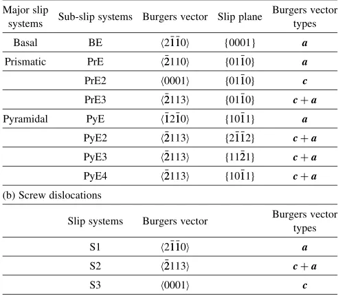
b2_CðmÞ _{is the measured b}2_{C of the sample. b represents} the magnitude of Burgers vector. Table 2 shows the most common slip systems in hexagonal crystals. There are three types of fundamental Burgers vectors represented asatype, ctype andcþatype in hexagonal crystals. In the analysis, therefore, averaged value of the magnitude of Burgers vector is used.b2_{represents the averaged value of squareb.}

b2_CðmÞ _{can be written as}9)

b2_CðmÞ_¼X

N

i¼1 fiC

ðiÞ

b2_i; ð2Þ

whereN is the number of different sub-slip systems. In the case of hexagonal crystals, N is equal to 11, as shown in Table 2.5)_CðiÞ _andb

i are the average contrast factor and the Burgers vector corresponding to theith sub-slip system, respectively. fi are the fractions of the particular sub-slip systems, where PN_i¼1fi¼1 and fi0. For a hexagonal crystal structure, eq. (2) can be written using three types of fundamental Burgers vectors, defined as b1 ¼1=3h2110i

(a type), b2¼1=3h0001i (c type) and b3 ¼1=3h2113i

(cþatype),

b2_C

hk:l

ðmÞ

¼b2₁X

Nhai

i¼1

fiCðiÞþb22

X Nhci

j¼1

fjCðjÞþb23

X Nhcþai

n¼1 fnCðnÞ;

ð3Þ

whereNhai,Nhci andNhcþai are the number of sub-slip systems with Burgers vector types a, c and cþa, respec-tively. The values of fi were determined by the relative fractions of the population of the Burgers vectors types,a,c and cþa, on the basis of the number of sub-slip systems. As a result, eq. (3) can be written as5,9)

b2_C

hk:l

ðmÞ

¼X

3

i¼1 hiC

ðiÞ

b2_i; ð4Þ

wherehiare the fractions of the dislocation population in the sample with the same Burgers vector,ba,bcandbcþa. Now,

CðiÞare the average contrast factors over the sub-slip systems

for the same Burgers vector types. Substituting eq. (1) in eq. (4), the following three equations are obtained:

qð₁mÞ¼1

P

X3

i¼1 hiChk:0

ðiÞ b2_iqð₁iÞ;

qð₂mÞ¼1

P

X3

i¼1 hiChk:0

ðiÞ

b2_iqð₂iÞ; ð5Þ

X3

i¼1 hi¼1;

where

P¼X

3

i¼1 hiChk:0

ðiÞ

b2_i ¼b2_C

hk:0 ðmÞ

; ð6Þ

0hi1: ð7Þ

q1ðmÞ and q2ðmÞ are the measured q1 and q2, respectively, which are determined from the modified Williamson–Hall plot mentioned in section 2.2. They can be obtained from the XRD profiles. Chk:0

ðiÞ

, q1ðiÞ _{and q2}ðiÞ _{are the numerically} calculated values for all sub-slip systems.

To evaluate the three unknowns,ha,hcandhcþathe values of the abovementioned parametersChk:0

ðiÞ

,q1ðiÞ _andq2ðiÞ _are required for solving the simultaneous equations of eq. (5). They were published previously for the most common sub-slip systems.9)Using the average values ofha,hc andhcþa,

b2_{Ccan be determined from eq. (6).}

2.2 Calculation of the values of q1ðmÞ and q2ðmÞ by the

modifiedWilliamson–Hall plot

The value of the full width at half-maximum (FWHM) obtained from each peak is substituted into the following modifiedWilliamson–Hall equation:10)

K¼0:9

D þ

M2_b2

2

1=2

1=2KC1=2þOðK2CÞ; ð8Þ

where K¼2sin= and K¼2cosðÞ=. Here, ,

andare the FWHM, diffraction angle and wavelength of the X-rays, respectively. In the case of Cu, ¼0:15405nm.D,

andbare the average particle size, the dislocation density and the magnitude of the Burgers vector, respectively. M is a constant depending on both the effective outer cut-off radius of dislocations and the dislocation density. O stands for higher-order terms inKC1=2. Equation (8) is converted into the quadratic form, in which its high-order term becomes negligible. Modifying eq. (1) into the quadratic form, the following equation is obtained:

½ðKÞ2=K2¼Chk:0ð1þq1xþq2x2Þ; ð9Þ

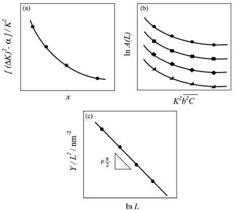
where¼ ð0:9=DÞ2 and¼M2_b2_{=2. The value of is} determined while keeping the left-hand side of eq. (9) as a quadratic function of x, as shown in Fig. 1(a). As a result, the measured values ofq1ðmÞ _andq2ðmÞ_{are obtained from the} coefficients ofxin the quadratic function.

2.3 Evaluation of the dislocation density by themodified

Warren–Averbach analysis

ThemodifiedWarren–Averbach equation is written as11) Table 2 The most common slip systems in hexagonal crystals.

(a) Edge dislocations

Major slip

systems Sub-slip systems Burgers vector Slip plane

Burgers vector types

Basal BE h211110i {0001} a

Prismatic PrE h22110i f01110g a

PrE2 h0001i f01110g c

PrE3 h22113i f01110g cþa

Pyramidal PyE h112110i f10111g a

PyE2 h22113i f211112g cþa

PyE3 h22113i f11221g cþa

PyE4 h22113i f10111g cþa

(b) Screw dislocations

Slip systems Burgers vector Burgers vector types

S1 h211110i a

S2 h22113i cþa

lnAðLÞ ¼lnASðLÞ b

2

2 L

2_ln Re

L ðK 2_CÞ

þQ b

2

2

2

L4ln R1

L ln R2

L ðK

4_C2_{Þ: ð10Þ}

For hexagonal crystals, eq. (10) can be arranged as

lnAðLÞ ¼lnASðLÞ

2L

2_ln Re L ðK

2_b2_CÞ

þQ

2

2

L4ln R1

L ln R2

L ðK

4_b2_C2_{Þ: ð11Þ}

Here, AðLÞis the real part of the Fourier coefficients of the XRD profiles. SuperscriptSin the termlnAðLÞindicates the crystallite size, andLis the Fourier variable.Lis defined as12)

L¼na3; ð12Þ

wherea3¼=f2ðsin2sin1Þg,nare integers starting from 0 and (21) is the angular range of the measured diffraction profiles.12)Reis the effective outer cut-off radius of dislocations.Q,R1 andR2 are all constants.

lnAðLÞ can be considered as a function of K2b2_{C from} eq. (11), and hence the dislocation density is determined from the lnAðLÞ versus K2_b2_C

hk:0 ðmÞ

plot, as shown in Fig. 1(b), as the coefficient of the second term in eq. (11)Y, which is arranged as

Y L2 ¼

2lnRe

2lnL: ð13Þ

The value of is evaluated from the gradient of the linear relationship betweenY=L2_{andlnL, as shown in Fig. 1(c).}

3. Experimental Procedures

A sample of AX52 die-cast alloy was cut into the proper size and polished mechanically with emery papers down to #2000, followed by buff polishing with Al2O3 powders

down to 0.3mm. Further, electropolishing was performed to remove the extra dislocations introduced into the sample surface by the earlier mechanical polishing.

For the XRD analysis, the diffraction profiles of the (00.2), (10.1), (11.0), (20.0), (20.1) and (21.1) reflections were measured with a conventional diffractometer (Rigaku UltimaIV X-ray diffractometer), using Cu K1 and K2 radiation operating at 40 kV and 40 mA at a scan speed of 0.25_min1_.

In this study, themodifiedWilliamson–Hall as well as the modified Warren–Averbach plots were employed to obtain the microstructural details involved in dislocation densi-ty.9,10,13)In these plots, the peaks obtained from only Cu K1 radiation were needed. Therefore, each peak was separated into K1radiation and K2radiation using a Lorenz function, and the FWHM of all peaks were obtained. A representative result of peak deconvolution is shown in Fig. 2.

4. Results and Discussion

The XRD profile data obtained from AX52 alloy are listed in Table 3. Using these data, analysis was performed according to eqs. (8) and (9). As a result, ¼4:29

105nm2,q1ðmÞ _{¼ 0:266andq2}ðmÞ_{¼0:0184are obtained} from the½ðKÞ2=K2 versusxplot, as shown in Fig. 3. Although the plot data is localised, a smooth quadratic curve was obtained.

From the value of , the average particle size Dcan be determined as:D¼137nm. The value ofDis apparent grain Fig. 1 Schematic diagrams showing the method of analysis: (a)½ðKÞ2

=K2_{versusxplot following eq. (9); (b) themodifiedWarren–Averbach}

plot following eq. (11); (c)Y=L2_versuslnL.

Fig. 2 Measured data and deconvolution lines using a Lorenz function of the (21.1) reflection.

Table 3 The diffraction angles and FWHM of the diffraction profiles used in this study.

Bragg reflections 2/deg FWHM/deg

00.2 34.47 3:97102

10.1 36.76 4:32102

11.0 57.71 6:22102

20.0 67.50 7:17102

20.1 70.20 7:46102

size measured from themodifiedWilliamson–Hall plot. This value reflects the grain size but is not always identical to the real size. Therefore, it should be considered to be a measure of the grain size.14)

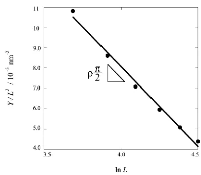
The values of q1ðmÞ _andq2ðmÞ _{are substituted into eq. (5),} and then the fractionshiof the three Burgers vector types are determined:ha¼0:84,hc¼0:10andhcþa¼0:06. Usinghi, themodifiedWarren–Averbach plot was prepared according to eq. (11). The result is shown in Fig. 4. A series of quadratic curves was obtained using several Lvalues. As a result,¼5:31013_m2_andR

e¼152nm were estimated, as shown in Fig. 5.

To discuss the validity of the results obtained in this study and the method employed, values reported previously on the dislocation density of magnesium alloys1,4) _{are listed in}

Table 4, together with the value obtained in this study. Itoh et al.reported the dislocation density of AX52 die-cast alloy,1) _{which is the same alloy used in this study.}

They measured the density with TEM techniques, and their reported value of is smaller than that of this study. In general, it is known that some dislocations leave the specimen surface, and a dislocation-free zone is formed in a very thin layer at the surface. The thickness of conventional TEM samples is roughly several tens of nm; hence, as

mentioned in section 1, the dislocation-free zone affects the number of dislocations and results in low density. Further-more, in TEM contrasts, it is not necessarily the case that all dislocations can be measured, because of the extinction law in TEM observations. The true value of in the sample must be larger than that reported by Itoh et al. With this interpretation, our result is consistent with the earlier results obtained by TEM observation and is considered to be practicable.

Ma´this et al. calculated the dislocation density of AZ91 alloys heat treated for 18 h at 686 K4)by XRD analysis. Their reported value ofis very close to that in this study. They used the MWP fitting procedure, which is the principal analysis method for obtaining the value of the dislocation density from XRD profiles.2)_{Although the alloy used in this}

study, AX52 is different in chemical composition from AZ91, the reported value is in good agreement with our result. Therefore, we conclude that the modified Warren– Averbach analysis is effective because of its simplicity and no arbitrary input data compared to the MWP fitting method.

5. Conclusion

The modified Warren–Averbach analysis method was revised and applied to the estimation of the dislocation density value in AX52 (Mg-Al-Mn-Ca) die-cast alloy from XRD profiles, and the validity of this analysis method was Fig. 3 The relationship between½ðKÞ2=K2_{andxin eq. (9).}

Fig. 4 ThemodifiedWarren–Averbach plot following eq. (11).

Fig. 5 Y=L2 _{versuslnLplot according to eq. (13). The gradient of the}

regression line provides the dislocation density. The effective outer cut-off radius of dislocations is also obtained from the intercept value of the horizontal scale.

Table 4 The comparison between the result of this study and others.

Specimen Method of analysis

Dislocation density

=1013_m2

This

study AX52 die-cast alloy

modifiedWarren-Averbach

plot 5.3

Itoh’s

study AX52 die-cast alloy TEM observation 2.0

Mathis’s study

AZ91 alloy (heat treated 18 h

at 686 K)

discussed. We found that this method is credible and accurate. A similar procedure using AX52 (Mg-Al-Mn-Ca) die-cast alloy in this study is also applicable to other hexagonal crystals, such as Ti, Zr and Zn, as well as MWP fitting.

Acknowledgement

This work was supported by Grant-in-Aid for Scientific Research of Japan Society for the Promotion of Science (JSPS), Japan.

REFERENCES

1) D. Itoh, Y. Terada and T. Sato: Mater. Trans.49(2008) 1957–1962. 2) G. Riba´rik, T. Unga´r and J. Gubicza: J. Appl. Cryst.34(2001) 669–

676.

3) K. Ma´this, K. Nyilas, A. Axt, I. Dragomir-Cernatescu, T. Unga´r and P.

Luka´cˇ: Acta Mater.52(2004) 2889–2894.

4) K. Ma´this, J. Gubicza and N. H. Nam: J. Alloy. Compd.394(2005) 194–199.

5) I. C. Dragomir, D. S. Li, G. A. Castello-Branco, H. Garmestani, R. L. Snyder, G. Riba´rik and T. Unga´r: Mater. Charact.55(2005) 66–74. 6) T. Unga´r, M. G. Glavicic, L. Balogh, K. Nyilas, A. A. Salem, G.

Riba´rik and S. L. Semiatin: Mater. Sci. Eng. A493(2008) 79–85. 7) T. Unga´r, O. Castelnau, G. Riba´rik, M. Drakopoulos, J. L. Be´chade, T.

Chauveau, A. Snigirev, I. Snigireva, C. Schroer and B. Bacroix: Acta Mater.55(2007) 1117–1127.

8) T. Unga´r, J. Gubicza, G. Riba´rik and A. Brobe´ly: J. Appl. Cryst.34

(2001) 298–310.

9) I. C. Dragomir and T. Unga´r: J. Appl. Cryst.35(2002) 556–564. 10) T. Unga´r and G. Tichy: Phys. Status. Solid.171(1999) 425–434. 11) T. Unga´r and A. Borbe´ly: Appl. Phys. Lett.69(1996) 3173–3175. 12) T. Kunieda, M. Nakai, Y. Murata, T. Koyama and M. Morinaga: ISIJ

Int.45(2005) 1909–1914.

13) T. Unga´r, J. Gubicza, G. Riba´rik and A. Borbe´ly: J. Appl. Cryst.34

(2001) 298–310.