A Kernel Independence Test for Geographical Language Variation

Language Variation

Dong Nguyen

Jacob Eisenstein

Georgia Institute of Technology

Quantifying the degree of spatial dependence for linguistic variables is a key task for analyzing dialectal variation. However, existing approaches have important drawbacks. First, they are based on parametric models of dependence, which limits their power in cases where the underly-ing parametric assumptions are violated. Second, they are not applicable to all types of lunderly-inguistic data: Some approaches apply only to frequencies, others to boolean indicators of whether a linguistic variable is present. We present a new method for measuring geographical language variation, which solves both of these problems. Our approach builds on Reproducing Kernel Hilbert Space (RKHS) representations for nonparametric statistics, and takes the form of a test statistic that is computed from pairs of individual geotagged observations without aggregation into predefined geographical bins. We compare this test with prior work using synthetic data as well as a diverse set of real data sets: a corpus of Dutch tweets, a Dutch syntactic atlas, and a data set of letters to the editor in North American newspapers. Our proposed test is shown to support robust inferences across a broad range of scenarios and types of data.

1. Introduction

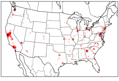
Figure 1 shows the geographical location of 1,000 Twitter posts containing the word hella, an intensifier used in expressions like I got hella studying to do and my eyes got hella big(Eisenstein et al. 2014). Although the word appears in major population centers throughout the United States, the map suggests that it enjoys a particularly high level of popularity on the west coast, in the area around San Francisco. But does this represent a real geographical difference in American English, or is it the result of chance fluctuation in a finite data set?

Regional variation of language has been extensively studied in sociolinguistics and dialectology (Lee and Kretzschmar, Jr. 1993; Chambers and Trudgill 1998; Grieve, Speelman, and Geeraerts 2011, 2013; Szmrecsanyi 2012; Nerbonne and Kretzschmar, Jr. 2013). A common approach involves mapping the geographic distribution of a linguistic variable (e.g., the choice ofsoda,pop, or coke to refer to a soft drink) and identifying boundaries between regions based on the data. The identification of linguistic variables that exhibit regional variation is therefore the first step in many studies of regional

∗E-mail:[email protected].

Submission received: 25 January 2016; revised version received: 29 August 2016; accepted for publication: 31 January 2017.

Figure 1

A map of 1,000 geolocated tweets containing the wordhella.

dialects. Traditionally, this step has been based on the manual judgment of the re-searcher; depending on the quality of the researcher’s intuitions, the most interesting or important variables might be missed.

The increasing amount of data available to study dialectal variation suggests a turn towards data-driven alternatives for variable selection. For example, researchers can mine social media data such as Twitter (Eisenstein et al. 2010; Doyle 2014; Huang et al. 2016) or product reviews (Hovy, Johannsen, and Søgaard 2015) to identify and test thousands of dialectal variables. Despite the large scale of available data, the well-known “long tail” phenomenon of language ensures that there will be many potential variables with low counts. A statistical metric for comparing the strength of geographi-cal associations across potential linguistic variables would allow linguists to determine whether finite geographical samples—such as the one shown in Figure 1—reveal a statistically meaningful association.

The use of statistical methods to analyze spatial dependence has been only lightly studied in sociolinguistics and dialectology. Existing approaches use classical statistics such as Moran’s I (e.g., Grieve, Speelman, and Geeraerts 2011), join count analysis (e.g., Lee and Kretzschmar Jr. 1993), and the Mantel Test (e.g., Scherrer 2012); we review these statistics in Section 2. These classical approaches suffer from a common problem: Each type of test can capture only a specific parametric form of spatial linguistic variation. As a result, these tests can incorrectly fail to reject the null hypothesis if the nature of the geolinguistic dependence does not match the underlying assumptions of the test.

To validate this approach, we compare it against three alternative spatial statistics: Moran’s I, the Mantel test, and join count analysis. For a controlled comparison, we use synthetic data to simulate different types of regional variation, and different types of linguistic data. This allows us to measure the capability of each approach to recover true geolinguistic associations, and to avoid type I errors even in noisy and sparse data. Next, we apply these approaches to three real linguistic data sets: a corpus of Dutch tweets, a Dutch syntactic atlas, and letters to the editor in North American newspapers.

To summarize, the contributions of this article are:

• We show how the Hilbert-Schmidt Independence Criterion can be applied to linguistic data. HSIC is a nonparametric test statistic that can handle both frequency and categorical data. It requires no discretization of geographic data, and is capable of detecting arbitrary geolinguistic dependencies (Section 3).

• We use synthetic data to compare the power and calibration of HSIC against three alternatives: Moran’s I, the Mantel Test, and join count analysis (Section 4).

• We apply these methods to analyze dialectal variation in three empirical data sets, in both English and Dutch, across a variety of registers

(Section 5).

2. Prior Work

This section describes prior work on global methods for quantifying the degree of spatial dependence in a geotagged corpus.1_{Although other global spatial statistics exist,}

we focus on the following three methods because they have been used in previous work on dialect analysis: Moran’s I (Grieve, Speelman, and Geeraerts 2011), join count analysis (Lee and Kretzschmar, Jr. 1993), and the Mantel test (Scherrer 2012).

We define a consistent notation across methods. Letxi represent a scalar linguistic

observation for unit i∈ {1. . .n} (typically, the presence or frequency of a linguistic variable), and letyirepresent a corresponding geolocation. For convenience, we define

dijas the spatial distance betweenyiandyj. Suppose we havenobservations, so that the

dataD={(x1,y1), (x2,y2),. . ., (xn,yn)}. Our goal is to test the strength of association

betweenXandY, against the null hypothesis that there is no association.

2.1 Moran’s I

Grieve, Speelman, and Geeraerts (2011) introduced the use of Moran’s I (Moran 1950; Cliff and Ord 1981) in the study of dialectal variation. To define the statistic, let W={wij}i,j∈{1...n} represent a spatial weighting matrix, such that larger values of wij

1 Global methods test for dependence over the entire data set. In some cases, there will be local

dependence in a few “hot spots,” even when global dependence is not detected, and local autocorrelation statistics have been proposed to capture such dependences (Anselin 1995). For example, Grieve (2016)

uses the Getis-OrdGistatistic (Getis and Ord 1992) in his analysis of regional American English. Local

indicate greater proximity, and wii=0. In their application of Moran’s I to a corpus

of newspaper letters to the editor, Grieve et al. defineWas

wij=

(

1, dij< τ,i6=j

0, dij≥τ, ori=j

(1)

where τis some critical threshold (Grieve, Speelman, and Geeraerts 2011). When the spatial weighting matrix is defined in this way, Moran’s I can be seen as a statistic that quantifies whether observationsxiandxjare more similar whenwij=1 than when

wij=0.2

Moran’s I is based on a hypothesized autoregressive processX=ρWX+, where Xis a vector of the linguistic observationsx1,. . .xn, andis a vector of uncorrelated

noise. BecauseXandWare given, the estimation problem is to findρso as to minimize the magnitude of. To take a probabilistic interpretation, it is typical to assume that consists of independent and identically distributed normal random variables with zero mean (Ord 1975). Under the null hypothesis of no spatial dependence between the observations inX, we would haveρ=0. Note, however, that we may fail to reject the possibility thatρ=0 even in the presence of spatial dependence, if the form of this dependence is not monotonic or nonlinear inW.

Becauseρis difficult to estimate exactly (Ord 1975), Moran’s I is used as an approx-imation. It is computed as

I= Pn n

i(xi−x)2

Pn

i

Pn

j wij(xi−x)(xj−x)

Pn

i

Pn

j wij

(2)

wherex= 1

nPixi. The ratio on the left is the inverse of the variance ofX; the ratio on

the right corresponds to the covariance between pointsiandjthat are spatially similar. Thus, the statistic rescales a spatially reweighted covariance (the ratio on the right of Equation (2)) by the overall variance (the ratio on the left of Equation (2)), giving an estimate of the overall spatial dependence of X. A compact alternative notation is to rewrite the statistic in terms of the vector ofresiduals R={ri}i∈1...n, where the residual

ri=xi−x. This yields the form I= R

>_WR

R>_R , with R> indicating the transpose of the column vectorR, and withWassumed to be normalized so thatP

i,jwij=n. Moran’s I

values often lie between−1 and 1, but the exact range depends on the weight matrixW, and is theoretically unbounded (de Jong, Sprenger, and van Veen 1984).

In hypothesis testing, our goal is to determine the p-value representing the likeli-hood that a value of Moran’s I at least as extreme as the observed value would arise by chance under the null hypothesis. The expected value of Moran’s I in the case of no spatial dependence is − 1

n−1. Grieve et al. compute p-values from a closed-form

approximation of the variance under the null hypothesis of total randomization. A nonparametric alternative is to perform apermutation test, calculating the empirical p-value by comparing the observed test statistic against the values that arise across multiple random permutations of the original data.

2 The matrixWcan be defined in other ways. We can define a continuous-valued version ofWby setting

wij=exp(−γdij), withdijequal to the geographical distance between unitsiandj. Alternatively, we

could define a topological spatial weighting matrix by settingwij=1 whenjis one of theknearest

In either case, Moran’s I does not test the null hypothesis of no statistical de-pendence between the linguistic featuresXand the geo-coordinatesY. Rather, it tests whether the estimated value ofρ would be likely to arise if there were no such de-pendence. If the nature of the geolinguistic dependence defies the assumptions of the statistic, however, then we risk incorrectly failing to reject the null hypothesis, a type II error. Put another way, there are forms of strong spatial dependence for whichρ=0, such as non-monotonic spatial relationships. This risk can be somewhat ameliorated by careful choice of the spatial weighting matrixW, which could in theory account for non-linear or even non-monotonic dependencies. However, an exhaustive search for someWthat obtains a low p-value would clearly be an invalid hypothesis test, and so Wmust be fixedbeforeany test is performed. In some cases, the researcher may bring substantive insights to the determination ofW, and so the flexibility of Moran’s I in this sense could be regarded as a positive feature. But there is little theoretical guidance, and a poor selection ofWwill result in inflated type II error rates.

From a practical standpoint, Moran’s I is applicable to only some types of linguistic data. In the study of dialect,Xtypically represents the frequency or presence of some linguistic variable, such as the use ofsodaversuspop. We are unaware of applications of Moran’s I to variables with more than two possibilities (e.g.,soda,pop,coke). One possible solution would be to perform multiple tests, with each alternant pitted against all the others. But it is not clear how the p-values from these multiple tests should be combined. For example, selecting the minimum p-value across the alternants would mean that the null hypothesis would be more likely to be rejected for variables with more alternants; averaging the p-values across alternants would have the opposite problem.

2.2 Join Count Analysis

If the linguistic dataXconsist of discrete observations,join count analysisis another approach for detecting spatial dependence. For each pair of points (i,j), we compute wijδ(xi=xj), where δ(xi=xj) returns a value of 1 if xi and xj are identical, and 0

otherwise. As in Moran’s I,wijis an element of a spatial weighting matrix, which could

be binary or continuous. The global sum of the counts is computed as

num-agree=

n

X

i n

X

j

wij(xixj+(1−xi)(1−xj)) (3)

= X>WX+(1−X)>W(1−X) (4)

with X> indicating the transpose of the column vector X. Note the similarity to the numerator of Moran’s I, which can be written asR>WR. The number of agreements can be compared with its expectation under the null hypothesis, yielding a hypothesis test for global autocorrelation (Cliff and Ord 1981).

Join count analysis has been applied to the study of dialect by Lee and Kretzschmar, Jr. (1993), who take each linguistic observation xi∈ {0, 1} to be a

bi-nary variable indicating the presence or absence of a dialect feature. They then build a binary spatial weighting matrix by performing a Delaunay triangulation over the geolocations of participants in dialect interviews, with wij=1 if the edge (i,j)

in low-density regions, the edges will be long. The method is therefore arguably more suitable to data in which the density of observations is highly variable—for example, between densely populated cities and sparsely populated hinterlands.

Because join count statistics are based on counts of agreements, this form of anal-ysis requires that each xi is a categorical variable—possibly non-binary—rather than

a frequency. In this sense, it is the complement of Moran’s I, which can be applied to frequencies, but not to non-binary discrete variables. Thus, join count analysis is best suited to cases where observations correspond to individual utterances (e.g., Twitter data, dialect interviews), rather than cases where observations correspond to longer texts (e.g., newspaper corpora).

2.3 The Mantel Test

The Mantel test can in principle be used to measure the dependence between any two arbitrary signals. In this test, we computedistancesfor each pair of linguistic variables, dx(xi,xj), and each pair of spatial locations,dy(yi,yj), forming a pair of distance matrices

Dx and Dy. We then estimate the element-wise correlation (usually, the Pearson

cor-relation) between these two matrices. Scherrer (2012) uses the Mantel test to correlate linguistic distance with geographical distance, and Gooskens and Heeringa (2006) cor-relate perceptual distance with linguistic distance. The Mantel test has also been applied to non-human dialect analysis, revealing regional differences in the call structures of Amazonian parrots by computing a linguistic distance matrixDxdirectly from spectral

measurements (Wright 1996).

Because it is built around distance functions, the Mantel test is applicable to binary, categorical, and frequency data—any kind of data for which a distance function can be constructed. For spatial locations, a typical choice is to compute the distance matrix based on the Euclidean distance between each pair of points. For binary or categorical linguistic data, the entries of the linguistic distance matrix can be set to 0 ifxi=xj, and

1 otherwise. For linguistic frequency data, we use the absolute difference between the frequency values.

The role of hypothesis testing in the Mantel test is to determine the likelihood that the observed test statistic—in this case, the correlation between the distance matrices DxandDy—could have arisen by chance under the null hypothesis. In the ideal case of

2.4 Other Related Work

Several computational studies have attempted to characterize linguistic differences across geographical regions, although most of these studies do not perform hypothesis testing on geographical dependence. A common approach is to aggregate geotagged social media content into geographical bins. Some studies rely on politically defined units such as nations and states (Hovy, Johannsen, and Søgaard 2015); however,

isoglosses (the geographical boundaries between linguistic features) need not align

with politically defined geographical units (Nerbonne and Kretzschmar, Jr. 2013). Other approaches rely on automatically defined geographical units, induced by computa-tional methods such as geodesic grids (Wing and Baldridge 2011), KD-trees (Roller et al. 2012), Gaussians (Eisenstein et al. 2010), and mixtures of Gaussians (Hong et al. 2012). While these approaches offer insights about the nature of geographical language variation, they do not provide test statistics that allow us to quantify the geographical dependence of various linguistic features.

As described in the next section, our approach is based on Reproducing Kernel Hilbert Spaces, which enable us to nonparametrically compare probability distribu-tions. Another way in which kernel methods can be applied to spatial analysis is in Gaussian Processes, which are often used to represent spatial data (Cressie 1988; Ecker and Gelfand 1997). Specifically, we can define a kernel over space, so that a response variable is distributed as a Gaussian with covariance defined by the kernel function. For example, it might be possible to model the popularity of linguistic features as a Gaussian Process, using the spatial covariance kernel to make smooth predictions at unknown locations. Our approach in this article is different, as we are interested in hypothesis testing, rather than modeling and prediction. Another difference is that we apply kernels to both the geographical and linguistic data sources, whereas a Gaussian Process approach would make the parametric assumption that the linguistic signal is Gaussian distributed with covariance defined by the spatial covariance kernel.

3. Hilbert-Schmidt Independence Criterion

Moran’s I, join count analysis, and the Mantel test share an important drawback: They do not directly test the independence of language and geography, but rather, they test for autocorrelation between X and Y, or between distances on these variables. Moran’s I tests whether the parameter of a linear autoregressive model is nonzero; the Mantel test is performed on the correlations between pairwise distances; join count statistics enable tests of whether spatially adjacent units tend to have the same linguistic features. In each case, rejection of the null hypothesis implies dependence between the geographical and linguistic signals. However, each test can incorrectly fail to reject the null hypothesis if its assumptions are violated, even if given an arbitrarily large amount of data.

We propose an alternative approach: directly test for the independence of geo-raphical and linguistic variables,PXY=? PXPY. Our approach, which is based on the

HSIC (Gretton et al. 2005a, 2008), makes no parametric assumptions about the form of these distributions. The proposed test isconsistent, in the sense that it will always reach the right decision, if provided enough data (Fukumizu et al. 2007).3

To test independence for arbitrary distributions PXY,PX, and PY, HSIC uses the

framework of RKHS. This framework will be familiar to the computational linguistics community through its application to support vector machines (Collins and Duffy 2001; Lodhi et al. 2002), wherekernel similarity functionsbetween pairs of instances are used to induce classifiers with highly non-linear decision boundaries. HSIC is a kernelized independence test, and it offers an analogous advantage: By computing kernel similar-ity functions on pairs of observations, it is possible to implicitly compare probabilsimilar-ity distributions across high-order moments, enabling nonparametric independence tests that are statistically consistent. An additional advantage of the RKHS framework is that it can be applied to arbitrary linguistic data—including dichotomous, polytomous, con-tinuous, and vector-valued observations—as long as an appropriate kernel similarity function can be defined.

Intuitively, HSIC tests independence by approximating a measure of the discrep-ancy between the joint geolinguistic distributionPXYand the product of independent

distributions PXPY. The forms of these distributions are unknown; for example, PY

might be Gaussian, or it might be some complicated multimodal distribution. The maximum mean discrepancy is a scalar function of the discrepancy between a pair of distributions, which makes no assumption about the distributions’ parametric forms. The maximum mean discrepancy will be large when linguistic similarity tends to co-occur with geographical similarity, indicating an association between language and geography that is unlikely to arise by chance. The key insight is that it is possible to approximate the maximum mean discrepancy from a finite sample of observations, by rewriting it as a sum of kernel similarity functions. These kernel functions should quantify the similarity between each pair of instances as a scalar; they must also obey some more technical properties, enumerated in Section 3.3. If the kernel functions are appropriately chosen, then the approximation is asymptotically consistent, meaning that it will approach the exact maximum mean discrepancy in the limit of infinite data, regardless of the forms ofPX,PY, and PXY. (This property is not shared by the

Mantel test, which is superficially similar in that it operates on distances between pairs of observations.) We now present the mathematical details of the method.

3.1 Comparing Probability Distributions

Themaximum mean discrepancy(MMD) is a nonparametric statistic that compares two

arbitrary probability distributions. In the HSIC test, this statistic is used to compare the joint distributionPXYwith the product of marginal distributionsPXPY. TheMMDis

defined as

MMD(P,Q)=sup

f

(EP[f(X)]−EQ[f(Y)]) (5)

where we take the supremum f over a set of possible functions, and compute the difference in the expected values under the distributions P and Q. Clearly, ifP=Q, thenMMD=0, but the challenge is to estimateMMDfor arbitraryPandQ, based only on finite samples from these distributions.

To explain how to do this, we introduce some concepts from RKHS. Let k:X×

X 7→R+denote a kernel function, mapping from pairs of observations (xi,xj) to reals.

A classical example is theradial basis function(RBF) kernel on vectors, wherek(xi,xj)=

exp −γ||xi−xj||22

For any instance x, the kernel function k defines a corresponding feature map

k(·,x) :X 7→_R+, which is the function that arises by fixing one of the arguments of the kernel function to the valuex. The “reproducing” property of RKHS implies an identity between kernel functions and inner products of feature maps:

k(xi,xj)=hk(·,xi),k(·,xj)i (6)

Thus, even though the feature map may be an arbitrarily complex function ofx, we can compute inner products of feature maps by computing the kernel similarity func-tion over the associated instances. TheMMD can be expressed in terms of such inner products, and thus, can be computed in terms of kernel similarity functions.

For a probability measure P, the mean element of P is defined as the expected feature map,µ_P=EPk(·,x). TheMMDcan then be computed in terms of kernel functions

of the mean elements,

MMD2(P,Q)=hµ_P,µ_Pi+hµ_Q,µ_Qi −2hµ_P,µ_Qi (7)

Ifµ_P=µ_Q, then theMMD is zero. The key observation is thatµ_P=µ_Qif and only ifP=Q, so long as an appropriate kernel similarity function is chosen (Fukumizu et al. 2007); see Section 3.3 for more on the choice of kernel functions.

Each of the inner products in Equation (7) corresponds to an expectation that can be estimated empirically from finite samples{x1,x2,. . .,xm}and{y1,y2,. . .,yn}:

MMD2(P,Q)= Ex,x0_∼Pk(x,x0)+_Ey,y0_∼Qk(y,y0)−2_Ex∼P,y∼Qk(x,y) (8)

\

MMD2(P,Q)= 1

m2

m

X

i,j

k(xi,xj)+ 1

n2

n

X

i,j

k(yi,yn)−_nm2 m

X

i=1

n

X

j=1

k(xi,yj) (9)

The full derivation is provided by Gretton et al. (2008). Having shown how to estimate a statistic on whether two probability measures are identical, we now use this statistic to test for independence.

3.2 Derivation of HSIC

To construct an independence test over random variablesXand Y, we test the MMD

between the joint distributionPXY and the product of marginalsPXPY. In this setting,

each observationicorresponds to a pair (xi,yi), so we require a kernel function on paired

observations,k((xi,yi), (xj,yj)). We define this as aproduct kernel,

k((xi,yi), (xj,yj))=kX(xi,xj)kY(yi,yj) (10)

wherekX andkYare kernels for the linguistic and geographic observations, respectively.

Using the product kernel, we can define mean embeddings for the distributions PXY andPXPY, enabling the application of the MMDestimator from Equation (9). The

Concretely, let us define theGram matrixKx so that (Kx)i,j=kX(xi,xj) for all pairs

i,jin the sample. Analogously, (Ky)i,j=kY(yi,yj). Then the HSIC can be estimated from

a finite sample ofmobservations as

\

HSIC= 1 n2

m

X

i,j

(Kx)i,j(Ky)i,j+ 1

n4

m

X

i,j,q,r

(Kx)i,j(Ky)q,r−_n2₃ m

X

i,j,q

(Kx)i,j(Ky)i,q (11)

= trKXHKYH

n2 (12)

wheretrindicates the matrix trace andHis a centering matrix,H=Im−1n11>. With

this definition ofH, we have

(KXH)ij= kX(xi,xj)−_n1

X

j0

kX(xi,xj0) (13)

(KYH)ij= kY(yi,yj)−_n1

X

j0

kY(yi,yj0) (14)

These two terms can be seen as mean-centered Gram matrices. By computing the trace of their matrix product, we obtain a cross-covariance between the Gram matrices. This trace is directly proportional to the maximum mean discrepancy betweenPXYand

PXPY. IfXandYare dependent, then large values ofkX(xi,xj) will imply large values

ofkY(yi,yj)—similar geography implies similar language—and so the cross-covariance

will be greater than zero. IfXandYare independent, then large values ofkX(xi,xj) are

not any more likely to correspond to large values ofkY(yi,yj), and so the expectation

of this cross-covariance will be zero.

3.3 Kernel Functions

To apply HSIC to the problem of detecting geolinguistic dependence, we must define the kernel functions kX andkY. In the RKHS framework, valid kernel functions must

be symmetric and positive semi-definite. To ensure consistency of the kernel-based estimator for MMD, the kernel must also be characteristic, meaning that it induces an injective mapping between probability measures and their corresponding mean elements (Fukumizu et al. 2007): Each probability measurePmust correspond to a single unique mean elementµ_P. Muandet et al. elaborate these and other properties of several well-known kernels (Muandet et al. 2016, Table 3.1).

For the spatial kernelkY, we use a Gaussian RBF, which is a widely used choice for

vector data. Specifically, we definekY(yi,yj;γ)=exp(−γd2i,j), where d2ij is the squared

Euclidean distance betweenyi andyj, andγis a parameter of the kernel function. We

also use the RBF inkX when the linguistic observations take on continuous values, such

as frequencies or phonetic data. The RBF kernel is symmetric, positive semi-definite, and characteristic.4

The parameterγcorresponds to the “length-scale” of the kernel. Intuitively, as this parameter increases, the kernel similarity drops off more quickly with distance. In this article, we follow the popular heuristic of settingγto the median of the data (y1,. . .yn),

as proposed by Gretton et al. (2005b). We empirically test the sensitivity of HSIC to this parameter in Section 4. More recent work offers optimization-based approaches for setting this parameter (Gretton et al. 2012), but we do not consider this possibility here.

Linguistic data are often binary or categorical. In this case, we use aDelta kernel

(also sometimes called a Dirac kernel). This kernel is simply defined askX(xi,xj)=1

if xi=xj and 0 otherwise. The Delta kernel has been used successfully in

combi-nation with HSIC for high-dimensional feature selection (Song et al. 2012; Yamada et al. 2014), and is symmetric, positive semi-definite, and characteristic for discrete data. For continuous or vector-valued linguistic variables, the RBF kernel can again be applied.

3.4 Scalability

The size of each Gram matrix is the square of the number of observations. For large data sets, this will be too expensive to compute. Following Gretton et al. (2005a), we use a low-rank approximation to each Gram matrix, using the incomplete Cholesky decomposition (Bach and Jordan 2002). Specifically, we approximate the symmetric matricesKX andKY as low-rank products,KX ≈AATandKY≈BBT, whereA∈Rn×rA

andB∈Rn×rB_{. The approximation quality is determined by the parametersr}

AandrB,

which are set to ensure that the magnitudes of the residualsK−AATandL−BBTare below a predefined threshold. HSIC may then be approximated as:

\

HSIC= trKXHKYH

n2 (15)

≈ tr(AA

T_)H(BBT_)H

n2 (16)

= tr(B

T_(HA))(BT_(HA))T

n2 (17)

where the matrix productHA can be computed without explicitly forming then×n matrixH, because of its simple structure. Alternative methods for scaling the computa-tion of HSIC are discussed in a recent note by Zhang et al. (2016).

4. Synthetic Data

We compare HSIC with specific instantiations of the methods described in Section 2, focusing on previous published applications of these methods to dialect analysis. Specifically, we consider the following methods:

Moran’s I We follow Grieve, Speelman, and Geeraerts (2011), using a binary spatial

weighting matrix with a distance thresholdτ, usually set to the median of the dis-tances between points in the data set.5_{This method is not applicable to categorical}

data.

Join counts We follow the approach of Lee and Kretzschmar, Jr. (1993), who define a

binary spatial weighting matrix from a Delaunay triangulation, and then compute join counts for linked pairs of observations. This method is not applicable to frequency data.

Mantel test We use Euclidean distance for the geographical distance matrix. For

con-tinuous linguistic data, we also use Euclidean distance; for discrete data, we use a delta function.

For all approaches, a one-tailed significance test is appropriate, because in nearly all conceivable dialectological scenarios we are testing only for the possibility that geo-graphically proximate units aremoresimilar than they would be under the null hypoth-esis. For some methods, it is possible to calculate a p-value from the test statistic using a closed form estimate of the variance. However, for consistency, we use a permutation approach to characterize the null distribution over the test statistic values. We permute the linguistic datax, breaking any link between geography and the language data, and then compute the distribution of the test statistic under many such permutations.

4.1 Data Generation

To ensure the verisimilitude of our synthetic data, we target the scenario of geotagged tweets in the Netherlands. For each municipality i, we stochastically determine the number and location of the tweets as follows:

Number of data points For each municipality, the number of tweetsniis chosen to be

proportional to the population, as estimated by Statistics Netherlands. Specifically, we draw ˜ni∼Poisson(µobs×populationi) and then setni=n˜i+1, ensuring that

each municipality has at least one data point. The parameter µ_obs controls the frequency of the linguistic variable. For example, a common orthographic variable (e.g., “g-deletion”) might have a high value ofµ_obs, whereas a rare lexical variable (e.g.,sodaversuspop) might have a much lower value. Note that µ_obs is shared across all municipalities.

Locations Next, for each tweet t, we determine the location yt by sampling without

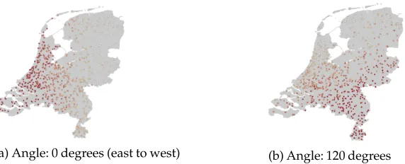
replacement from the set of real tweet locations in municipalityi(the data set is described in Section 5.3). This ensures that the distribution of geolocations in the synthetic data matches the real geographical distribution of tweets, rather than drawing from a parametric distribution that may not match the complexity of true geographical population distributions. Each location is represented as a latitude and longitude pair (Figure 2).

For each variable, each municipality is assigned a frequency vector θ_i, indicating the relative frequency of each variable form: for example 70% soda, 30%pop. We discuss

(a) Angle: 0 degrees (east to west) _{(b) Angle: 120 degrees}

Figure 2

Synthetic frequency data with dialect continua in two different angles.

methods for settingθ_isubsequently, which enable the simulation of a range of dialectal phenomena.

We simulate both counts data and frequency data. In counts data—such as geotagged tweets—the data points in each instance in municipalityiare drawn from a binomial or multinomial distribution with parameterθ_i. In frequency data, we observe only the relatively frequency of each variable form for each municipality. In this case, we draw the frequency from a Dirichlet distribution with expected value equal toθ_i, drawingφ_t∼Dirichlet(sθ_i), where the scale parameterscontrols the variance within each municipality.

4.2 Calibration

Our first use of synthetic data is to examine the p-values obtained from each method when the null hypothesis is true—that is, when there is no geographical variation in the data. The p-value corresponds to the likelihood of seeing a test statistic at least as extreme as the observed value, under the null hypothesis. Thus, if we repeatedly generate data under the null hypothesis, a well-calibrated test will return a distribution of p-values that is uniform in the interval [0, 1]. We would expect to observe p<0.05 in exactly 5% of cases, corresponding to the allowed rate of type I errors (incorrect rejection of the null hypothesis) at the thresholdα=0.05.

To measure the calibration of each of the proposed tests, we generate 1,000 ran-dom data sets using this procedure, and then compute the p-values under each test. In these random data sets, the relative frequency parametersθ_i are the same for all municipalities, which is the null hypothesis of complete randomization. To generate the binary and categorical data, we useµ_obs=10−5, meaning that the expected number of observations is 1 per 100, 000 individuals in the municipality; for comparison, this corresponds roughly to the tweet frequency of the lengthened spelling hellla in the 2009–2012 Twitter data set gathered by Eisenstein et al. (2014).

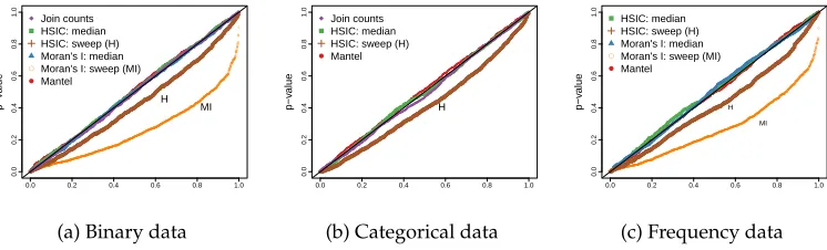
To visualize the calibration of each test, we use quantile-quantile (Q-Q) plots, com-paring the obtained p-values with a uniform distribution. A well-calibrated test should give a diagonal line from the origin to (1, 1). Figure 3 shows the Q-Q plots obtained from each method on each relevant type of data (recall that not all methods can be applied to all types of data, as described in the previous section).

●●●●●●●●●●●●●●●●●●●●●●●●●●●●●●●●●●●●●●●●●●●●●●●●●●●●●●●●●●●●●●●●●●●●●●●●●●●●●●●●●●●●●●●●●●●●●●●●●●●●●●●●●●●●●●●●●●●●●●●●●●●●●●●●●●●●●●●●●●●●●●●●●●●●●●●●●●●●●●●●●●●●●●●●●●●●●●●●●●●●●●●●●●●●●●●●●●●●●●●●●●●●●●●●●●●●●●●●●●●●●●●●●●●●●●●●●●●●●●●●●●●●●●●●●●●●●●●●●●●●●●●●●●●●●●●●●●●●●●●●●●●●●●●●●●●●●●●●●●●●●●●●●●●●●●●●●●●●●●●●●●●●●●●●●●●●●●●●●●●●●●●●●●●●●●●●●●●●●●●●●●●●●●●●●●●●●●●●●●●●●●●●●●●●●●●●●●●●●●●●●●●●●●●●●●●●●●●●●●●●●●●●●●●●●●●●●●●●●●●●●●●●●●●●●●●●●●●●●●●●●●●●●●●●●●●●●●●●●●●●●●●●●●●●●●●●●●●●●●●●●●●●●●●●●●●●●●●●●●●●●●●●●●●●●●●●●●●●●●●●●●●●●●●●●●●●●●●●●●●●●●●●●●●●●●●●●●●●●●●●●●●●●●●●●●●●●●●●●●●●●●●●●●●●●●●●●●●●●●●●●●●●●●●●●●●●●●●●●●●●●●●●●●●●●●●●●●●●●●●●●●●●●●●●●●●●●●●●●●●●●●●●●●●●●●●●●●●●●●●●●●●●●●●●●●●●●●●●●●●●●●●●●●●●●●●●●●●●●●●●●●●●●●●●●●●●●●●●●●●●●●●●●●●●●●●●●●●●●●●●●●●●●●●●●●●●●●●●●●●●●●●●●●●●●●●●●●●●●●●●●●●●●●●●●●●●●●●●●●●●●●●●●●●●●●●●●●●●●●●●●●●●●●●●●●●●●●●●●●●●●●●●●●●●●●●●●●●●●●●●●●●●●●●●●●●●●●●●●●●●●●●●●●●●●●●●●●●●●●●●●●●●●●●●●●●● ●●●●●●●●●●●●●●●●●●●●●●●●●●●●●●●●● ●●●●●●●●● ●●● ●● ●

0.0 0.2 0.4 0.6 0.8 1.0

0.0 0.2 0.4 0.6 0.8 1.0 p−v alue ● ● ●●●●●●●●●●●●●●●●●●●●●●●●●●●●●●●●●●●●●●●●●●●●●●●●●●●●●●●●●●●●●●●●●●●●●●●●●●●●●●●●●●●●●●●●●●●●●●●●●●●●●●●●●●●●●●●●●●●●●●●●●●●●●●●●●●●●●●●●●●●●●●●●●●●●●●●●●●●●●●●●●●●●●●●●●●●●●●●●●●●●●●●●●●●●●●●●●●●●●●●●●●●●●●●●●●●●●●●●●●●●●●●●●●●●●●●●●●●●●●●●●●●●●●●●●●●●●●●●●●●●●●●●●●●●●●●●●●●●●●●●●●●●●●●●●●●●●●●●●●●●●●●●●●●●●●●●●●●●●●●●●●●●●●●●●●●●●●●●●●●●●●●●●●●●●●●●●●●●●●●●●●●●●●●●●●●●●●●●●●●●●●●●●●●●●●●●●●●●●●●●●●●●●●●●●●●●●●●●●●●●●●●●●●●●●●●●●●●●●●●●●●●●●●●●●●●●●●●●●●●●●●●●●●●●●●●●●●●●●●●●●●●●●●●●●●●●●●●●●●●●●●●●●●●●●●●●●●●●●●●●●●●●●●●●●●●●●●●●●●●●●●●●●●●●●●●●●●●●●●●●●●●●●●●●●●●●●●●●●●●●●●●●●●●●●●●●●●●●●●●●●●●●●●●●●●●●●●●●●●●●●●●●●●●●●●●●●●●●●●●●●●●●●●●●●●●●●●●●●●●●●●●●●●●●●●●●●●●●●●●●●●●●●●●●●●●●●●●●●●●●●●●●●●●●●●●●●●●●●●●●●●●●●●●●●●●●●●●●●●●●●●●●●●●●●●●●●●●●●●●●●●●●●●●●●●●●●●●●●●●●●●●●●●●●●●●●●●●●●●●●●●●●●●●●●●●●●●●●●●●●●●●●●●●●●●●●●●●●●●●●●●●●●●●●●●●●●●●●●●●●●●●●●●●●●●●●●●●●●●●●●●●●●●●●●●●●●●●●●●●●●●●●●●●●●●●●●●●●●●●●●●●●●●●●●●●●●●●●●●●●●●●●●●●●●●●●●●●●●●●●●●●●●●●●●●●●●●●●●●●●●●●●●●●●●●●●●●●●●● ● ● Join counts HSIC: median HSIC: sweep (H) Moran's I: median Moran's I: sweep (MI) Mantel

MI H

(a) Binary data

●●●●●●●●●●●●●●●●●●●●●●●●●●●●●●●●●●●●●●●●●●●●●●●●●●●●●●●●●●●●●●●●●●●●●●●●●●●●●●●●●●●●●●●●●●●●●●●●●●●●●●●●●●●●●●●●●●●●●●●●●●●●●●●●●●●●●●●●●●●●●●●●●●●●●●●●●●●●●●●●●●●●●●●●●●●●●●●●●●●●●●●●●●●●●●●●●●●●●●●●●●●●●●●●●●●●●●●●●●●●●●●●●●●●●●●●●●●●●●●●●●●●●●●●●●●●●●●●●●●●●●●●●●●●●●●●●●●●●●●●●●●●●●●●●●●●●●●●●●●●●●●●●●●●●●●●●●●●●●●●●●●●●●●●●●●●●●●●●●●●●●●●●●●●●●●●●●●●●●●●●●●●●●●●●●●●●●●●●●●●●●●●●●●●●●●●●●●●●●●●●●●●●●●●●●●●●●●●●●●●●●●●●●●●●●●●●●●●●●●●●●●●●●●●●●●●●●●●●●●●●●●●●●●●●●●●●●●●●●●●●●●●●●●●●●●●●●●●●●●●●●●●●●●●●●●●●●●●●●●●●●●●●●●●●●●●●●●●●●●●●●●●●●●●●●●●●●●●●●●●●●●●●●●●●●●●●●●●●●●●●●●●●●●●●●●●●●●●●●●●●●●●●●●●●●●●●●●●●●●●●●●●●●●●●●●●●●●●●●●●●●●●●●●●●●●●●●●●●●●●●●●●●●●●●●●●●●●●●●●●●●●●●●●●●●●●●●●●●●●●●●●●●●●●●●●●●●●●●●●●●●●●●●●●●●●●●●●●●●●●●●●●●●●●●●●●●●●●●●●●●●●●●●●●●●●●●●●●●●●●●●●●●●●●●●●●●●●●●●●●●●●●●●●●●●●●●●●●●●●●●●●●●●●●●●●●●●●●●●●●●●●●●●●●●●●●●●●●●●●●●●●●●●●●●●●●●●●●●●●●●●●●●●●●●●●●●●●●●●●●●●●●●●●●●●●●●●●●●●●●●●●●●●●●●●●●●●●●●●●●●●●●●●●●●●●●●●●●●●●●●●●●●●●●●●●●●●●●●●●●●●●●●●●●●●●●●●●●●●●●

0.0 0.2 0.4 0.6 0.8 1.0

0.0 0.2 0.4 0.6 0.8 1.0 p−v alue ● Join counts HSIC: median HSIC: sweep (H) Mantel

H

(b) Categorical data

●●●●●●●●●●●●●●●●●●●●●●●●●●●●●●●●●●●●●●●●●●●●●●●●●●●●●●●●●●●●●●●●●●●●●●●●●●●●●●●●●●●●●●●●●●●●●●●●●●●●●●●●●●●●●●●●●●●●●●●●●●●●●●●●●●●●●●●●●●●●●●●●●●●●●●●●●●●●●●●●●●●●●●●●●●●●●●●●●●●●●●●●●●●●●●●●●●●●●●●●●●●●●●●●●●●●●●●●●●●●●●●●●●●●●●●●●●●●●●●●●●●●●●●●●●●●●●●●●●●●●●●●●●●●●●●●●●●●●●●●●●●●●●●●●●●●●●●●●●●●●●●●●●●●●●●●●●●●●●●●●●●●●●●●●●●●●●●●●●●●●●●●●●●●●●●●●●●●●●●●●●●●●●●●●●●●●●●●●●●●●●●●●●●●●●●●●●●●●●●●●●●●●●●●●●●●●●●●●●●●●●●●●●●●●●●●●●●●●●●●●●●●●●●●●●●●●●●●●●●●●●●●●●●●●●●●●●●●●●●●●●●●●●●●●●●●●●●●●●●●●●●●●●●●●●●●●●●●●●●●●●●●●●●●●●●●●●●●●●●●●●●●●●●●●●●●●●●●●●●●●●●●●●●●●●●●●●●●●●●●●●●●●●●●●●●●●●●●●●●●●●●●●●●●●●●●●●●●●●●●●●●●●●●●●●●●●●●●●●●●●●●●●●●●●●●●●●●●●●●●●●●●●●●●●●●●●●●●●●●●●●●●●●●●●●●●●●●●●●●●●●●●●●●●●●●●●●●●●●●●●●●●●●●●●●●●●●●●●●●●●●●●●●●●●●●●●●●●●●●●●●●●●●●●●●●●●●●●●●●●●●●●●●●●●●●●●●●●●●●●●●●●●●●●●●●●●●●●●●●●●●●●●●●●●●●●●●●●●●●●●●●●●●●●●●●●●●●●●●●●●●●●●●●●●●●●●●●●●●●●●●●●●●●●●●●●●●●●●●●●●●●●●●●●●●●●●●●●●●●●●●●●●●●●●●●●●●●●●●●●●●●●●●●●●●●●●●●●●●●●●●●●●●●●●●●●●●●●●●●●● ●●●●●●●● ●●●●●●●●●● ●

0.0 0.2 0.4 0.6 0.8 1.0

0.0 0.2 0.4 0.6 0.8 1.0 p−v alue ●●●●●●●●●●●●●●●●●●●●●●●●●●●●●●●●●●●●●●●●●●●●●●●●●●●●●●●●●●●●●●●●●●●●●●●●●●●●●●●●●●●●●●●●●●●●●●●●●●●●●●●●●●●●●●●●●●●●●●●●●●●●●●●●●●●●●●●●●●●●●●●●●●●●●●●●●●●●●●●●●●●●●●●●●●●●●●●●●●●●●●●●●●●●●●●●●●●●●●●●●●●●●●●●●●●●●●●●●●●●●●●●●●●●●●●●●●●●●●●●●●●●●●●●●●●●●●●●●●●●●●●●●●●●●●●●●●●●●●●●●●●●●●●●●●●●●●●●●●●●●●●●●●●●●●●●●●●●●●●●●●●●●●●●●●●●●●●●●●●●●●●●●●●●●●●●●●●●●●●●●●●●●●●●●●●●●●●●●●●●●●●●●●●●●●●●●●●●●●●●●●●●●●●●●●●●●●●●●●●●●●●●●●●●●●●●●●●●●●●●●●●●●●●●●●●●●●●●●●●●●●●●●●●●●●●●●●●●●●●●●●●●●●●●●●●●●●●●●●●●●●●●●●●●●●●●●●●●●●●●●●●●●●●●●●●●●●●●●●●●●●●●●●●●●●●●●●●●●●●●●●●●●●●●●●●●●●●●●●●●●●●●●●●●●●●●●●●●●●●●●●●●●●●●●●●●●●●●●●●●●●●●●●●●●●●●●●●●●●●●●●●●●●●●●●●●●●●●●●●●●●●●●●●●●●●●●●●●●●●●●●●●●●●●●●●●●●●●●●●●●●●●●●●●●●●●●●●●●●●●●●●●●●●●●●●●●●●●●●●●●●●●●●●●●●●●●●●●●●●●●●●●●●●●●●●●●●●●●●●●●●●●●●●●●●●●●●●●●●●●●●●●●●●●●●●●●●●●●●●●●●●●●●●●●●●●●●●●●●●●●●●●●●●●●●●●●●●●●●●●●●●●●●●●●●●●●●●●●●●●●●●●●●●●●●●●●●●●●●●●●●●●●●●●●●●●●●●●●●●●●●●●●●●●●●●●●●●●●●●●●●●●●●●●●●●●●●●●●●●●●●●●●●●●●●●●●●●●●●●●●●●●●●●●●●●●●●●●●●●● ● ● HSIC: median HSIC: sweep (H) Moran's I: median Moran's I: sweep (MI) Mantel

MI H

(c) Frequency data

Figure 3

Quantile-quantile plots comparing the distribution of the obtained p-values with a uniform distribution. They-axis is the p-value returned by the tests. Thex-axis shows the corresponding quantile for a uniform distribution on the range [0,1]. The approaches that optimize the parameters, namely, the cutoff for Moran’s I (MI) and the bandwidth for HSIC (H), lead to a skewed distribution of p-values.

threshold for constructing the neighborhood matrixW; in HSIC, we use 1

d2 as the kernel

bandwidth parameter. Figure 3 shows that by basing these parameters on the median distance between pairs of points, we obtain well-calibrated results. However, some prior work takes an alternative approach, sweeping over parameter values to obtain the most significant results (Grieve, Speelman, and Geeraerts 2011). In our experiments we sweep across the distance cutoff for Moran’s I, and the bandwidth for the spatial distances in HSIC. This distorts the calibration, meaning that the resulting p-values are not reliable. This is most severe for Moran’s I with type I error rates of 11.7% (binary data) and 14.3% (frequency data) when the significance threshold α is set to 5%. Given that such parameter sweeps are explicitly designed to maximize the number of positive test results—and not the overall calibration of the test—this is unsurprising. We therefore avoid parameter sweeps in the remainder of this article, and rely instead on median distance as a simple heuristic alternative.

4.3 Power

Next, we consider synthetic data in which there is geographical variation by construc-tion. We assess thepowerof each approach by computing the fraction of simulations for which the approaches correctly rejected the null hypothesis of no spatial dependence, given a significance threshold ofα=0.05. We again use the Netherlands as the stage for all simulations, and consider two types of geographical variation.

Dialect continua We generate data such that the frequency of a linguistic variant

in-creases linearly through space, as in a dialect continuum (Heeringa and Nerbonne 2001). In most of the synthetic data experiments herein, we average across a range of angles, from 0◦to 357◦with step sizes of 3◦, yielding 120 distinct angles in total. Each angle aligns differently with the population distribution of the Netherlands, so we also assess sensitivity of each method to the angle itself. Figure 2 shows two synthetic data sets with dialect continua in different angles.

Geographical centers Second, we consider a setting in which variation is based on one

corresponds to the dialectological scenario in which a variable form is centered on one specific city, as in, say, the association of the wordhellawith the San Francisco metropolitan area. We average across 25 possible centers: the capitals of each of the 12 provinces of the Netherlands; the national capital of the Netherlands (Amsterdam); thetwomost populous cities in each of the 12 provinces. For each setting, we randomly generate synthetic data four times, resulting in a total of 100 synthetic data sets for this condition.

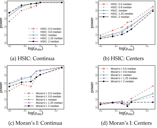
Parameter settings.We use these data generation scenarios to test the sensitivity of HSIC and Moran’s I to their hyperparameters, by varying the kernel bandwidths in HSIC (Figures 4a and 4b) and the distance threshold in Moran’s I (Figures 4c and 4d). The sensitivity of HSIC to the bandwidth value decreases as the number of data points increases (as governed byµ_obs), especially in the case of dialect continua. The sensitivity of Moran’s I to the distance cutoff value decreases with the amount of data in the case of dialect continua, but in the case of center-based variation, Moran’s I becomes moresensitive to this parameter as there is more data. For both methods, the same trends regarding the best performing parameters can be observed. In the case of dialect continua, larger cutoffs and bandwidths perform best, but in the case of variation based on centers, smaller cutoffs and bandwidths lead to higher power. Overall, there is no single best parameter setting, but the median heuristics perform reasonably well for both types of variation.

Direction of dialect continua.We simulate dialect continua by varying the frequency of linguistic variables linearly through space. Because of the heterogeneity of population density, different spatial angles will have very different properties: For example, one choice of angle would imply a continuum cutting through several major cities, whereas

−5.0 −4.5 −4.0 −3.5

0.0 0.2 0.4 0.6 0.8 1.0

log(µobs)

po w er ● ● ● ● ● ● ● ● ● ● ● ● ● ● ● ● ● ● ● ● ●

HSIC: 0.5 median HSIC: 0.8 median HSIC: median HSIC: 1.25 median HSIC: 2 median

(a) HSIC: Continua

−5.0 −4.5 −4.0 −3.5

0.0 0.2 0.4 0.6 0.8 1.0

log(µobs)

po w er ● ● ● ● ● ● ● ● ● ● ● ● ● ● ● ● ● ● ● ● ●

HSIC: 0.5 median HSIC: 0.8 median HSIC: median HSIC: 1.25 median HSIC: 2 median

(b) HSIC: Centers

−5.0 −4.5 −4.0 −3.5

0.0 0.2 0.4 0.6 0.8 1.0

log(µobs)

po w er ● ● ● ● ● ● ● ● ● ● ● ● ● ● ● ● ● ● ● ● ●

Moran's I: 0.5 median Moran's I: 0.8 median Moran's I: median Moran's I: 1.25 median Moran's I: 2 median

(c) Moran’s I: Continua

−5.0 −4.5 −4.0 −3.5

0.0 0.2 0.4 0.6 0.8 1.0

log(µobs)

po w er ● ● ● ● ● ● ● ● ● ● ● ● ● ● ● ● ● ● ● ● ●

Moran's I: 0.5 median Moran's I: 0.8 median Moran's I: median Moran's I: 1.25 median Moran's I: 2 median

(d) Moran’s I: Centers

Figure 4

0 50 100 150 200 250 300 350 0.0 0.2 0.4 0.6 0.8 1.0 Angle po w er ● ● ●● ● ● ● ●● ● ● ● ● ● ● ● ● ● ●_Mantel HSIC Moran's I Join counts Figure 5

Relationship between the statistical power of each test and the angle of the dialect continuum across the Netherlands.

another choice might imply a rural–urban distinction. Figure 5 shows the power of the methods on binary data (there are two variant forms, and each instance contains exactly one of them), in which we vary the angle of the continuum. HSIC is insensitive to the angle of variation, demonstrating the advantage of this kernel nonparametric method. Moran’s I is relatively robust, whereas join count analysis performs poorly across the entire range of settings. The Mantel test is remarkably sensitive to the angle of variation, attaining nearly zero power for some scenarios of dialect continua. This is caused by the complex interaction between the underlying linguistic phenomenon and the east–west variation of the population density of the Netherlands. For example, when the dialect continuum is simulated at an angle of 105 degrees, the southeast of the Netherlands has a higher usage of the variable, but this is only a very small region because of the shape of the country. The Mantel test apparently has great difficulty in detecting geographical variation in such cases.

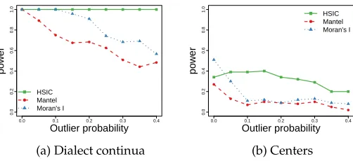
Outliers. In the frequency-based synthetic data, each instance uses each variable form with some continuous frequency—this is based on the scenario of letters to the editors of regional newspapers, as explored in prior work (Grieve, Speelman, and Geeraerts 2011). We test the robustness of each approach by introducing outliers: Randomly selected data points whose variable frequencies are replaced at random with extreme values of either 0 or 1. As shown in Figure 6, HSIC is the most robust against outliers, and the performance of the Mantel test is the most affected by outliers (recall that join count analysis applies only to discrete observations, so it cannot be compared on this measure).

0.0 0.1 0.2 0.3 0.4

0.0 0.2 0.4 0.6 0.8 1.0 Outlier probability po w er ● ● ● ● ● ● ● ● ● ● HSIC Mantel Moran's I

(a) Dialect continua

0.0 0.1 0.2 0.3 0.4

0.0 0.2 0.4 0.6 0.8 1.0 Outlier probability po w er ● ● ● ● ● ● ● ● ● ● HSIC Mantel Moran's I (b) Centers Figure 6

−5.0 −4.5 −4.0 −3.5 0.0 0.2 0.4 0.6 0.8 1.0

log(µobs)

po w er ● ● ● ● ● ● ● Join counts HSIC Mantel Moran's I

(a) Binary variable

−5.0 −4.5 −4.0 −3.5

0.0 0.2 0.4 0.6 0.8 1.0

log(µobs)

po w er ● ● ● ● ● ● ● Join counts HSIC Mantel

(b) Categorical variable

0.00 0.05 0.10 0.15

0.0 0.2 0.4 0.6 0.8 1.0 σ po w er ● ● ● ● ● ● ● ● HSIC Mantel Moran's I

(c) Frequency variable

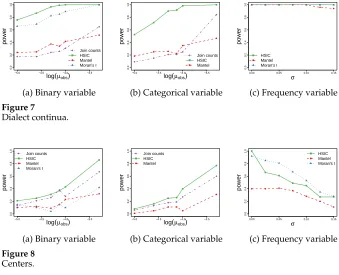
Figure 7

Dialect continua.

−5.0 −4.5 −4.0 −3.5

0.0 0.2 0.4 0.6 0.8 1.0

log(µobs)

po w er ● ● ● ● ● ● ● Join counts HSIC Mantel Moran's I

(a) Binary variable

−5.0 −4.5 −4.0 −3.5

0.0 0.2 0.4 0.6 0.8 1.0

log(µobs)

po w er ● ● ● ● ● ● ● Join counts HSIC Mantel

(b) Categorical variable

0.00 0.05 0.10 0.15

0.0 0.2 0.4 0.6 0.8 1.0 σ po w er ● ● ● ● ● ● ● ● HSIC Mantel Moran's I

(c) Frequency variable

Figure 8

Centers.

Overall.We now compare the methods by averaging across various settings simulating dialect continua (Figure 7) and variation based on centers (Figure 8). To generate the categorical data, we varyµ_obsin our experiments, with a higherµ_obsresulting in more tweets and consequently less variation on the municipality level. As expected, the power of the approaches increases asµ_obsincreases in the experiments on the categorical data, and the power of the approaches decreases asσincreases in the experiments on the frequency data. The experiments on the binary and categorical data show the same trends: HSIC performs the best across all settings. Join count analysis does well when the variation is based on centers, and Moran’s I does best for dialect continua. Moran’s I performs best on the frequency data, especially in the case of variation based on centers.

4.4 Summary

●

● ● ●

● ●

● ●

●

●

● ●

● ●

●

● ● ● ●

● ● ● ● ●

● ● ●

● ● ● ●

● ●

200 400 600 800 1000

0.20

0.25

0.30

0.35

Threshold (miles)

Propor

tion significant

Figure 9

The proportion of variables detected to be significant (p<0.05) by Moran’s I by varying the distance cutoff (without adjusting for multiple comparisons).

5. Empirical Data

We now assess the spatial dependence of linguistic variables on three real linguistic data sets: letters to the editor (English), a syntactic atlas of the Dutch dialects, and Dutch geotagged tweets. In each data set, we compute statistical significance for the geolinguistic dependence of multiple linguistic variables. To adjust the significance thresholds for multiple comparisons, we use the Benjamini-Hochberg procedure (Benjamini and Hochberg 1995) to bound the overall false discovery rate (FDR).

5.1 Letters to the Editor

In their application of Moran’s I to English dialects in the United States, Grieve, Speelman, and Geeraerts (2011) compile a corpus of letters to the editors of news-papers to measure the presence of dialect variables in text. To compute the frequency of the lexical variables, letters are aggregated to core-based statistical areas, which are defined by the United States to capture the geographical region around an urban core. The frequency of 40 manually selected lexical variables is computed for each of 206 cities.

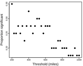
We use the Mantel test, HSIC, and Moran’s I to assess the spatial dependence of variables in this data set. Join count analysis was excluded, because it is not suitable for frequency data. We verified our implementation of Moran’s I by following the approach taken by Grieve et al.: we computed Moran’s I for cutoffs in the range of 200 to 1,000 miles and selected the cutoff that yielded the lowest p-value. The ob-tained cutoffs and test statistics closely followed the values reported in the analysis by Grieve et al., with slight deviations possibly due to our use of a permutation test rather than a closed-form approximation to compute the p-values.

After adjusting the p-values using the FDR procedure, a 500-mile cutoff results in three significant linguistic variables.6 _{However, recall that the approach of selecting}

parameters by maximizing the number of positive test results tends to produce a large number of type I errors. When setting the distance cutoff to the median distance between data points, none of the linguistic variables were found to have a significant geographical association. Similarly, HSIC and the Mantel test also found no significant associations after adjusting for multiple comparisons. Figure 9 shows the proportion of

Table 1

Highest ranked variables by HSIC. All methods had an adjusted p-value<0.05 for all variables, except variable 2:30b (Mantel: p=0.118.

Map id Description

1:84b Free relative, complementizer following relative pronoun 1:84a Short subject and object relative,

complementizer following relative pronoun

1:80b ONE pronominalization

1:33a Complementizer agreement 3 plural 1:76a Reflexive pronouns; synthesis 2:36b Form of the participle of

the modal verb willen ‘want’ 1:29a Complementizer agreement 1 plural 1:69a Correlation weak reflexive pronouns 2:30b Interruption of the verbal cluster;

synthesis I

2:61a Forms for iemand ‘somebody’

Figure 10

SAND map 16b, book 1.

Finite complementizer(s) following relative pronoun (N = 112). HSIC: p = 0.024; Mantel: p = 0.506; Join counts: p = 0.002.

significant variables according to Moran’s I based on different thresholds. The numbers vary considerably depending on the threshold. The figure also suggests that the median distance (921 miles) may not be a suitable threshold for this data set.

5.2 Syntactic Atlas of the Dutch Dialects (SAND)

Dialect atlases are frequently used in the study of dialect. In this section we demonstrate the use of the discussed methods on SAND (Barbiers et al. 2005, 2008), an online elec-tronic atlas that maps syntactic variation of Dutch varieties in the Netherlands, Belgium, and France.7 The data were collected between the years of 2000 and 2005. SAND has been used to measure the distances between dialects, and to discover dialect regions (Spruit 2006; Tjong Kim Sang 2015). To our knowledge, we are the first to use statistical methods to quantify the degree of spatial dependence of the linguistic variables in this atlas. Compared with the other empirical data sets that we consider, this data set is smaller and many variables contain more than two variants.

In our experiments, we consider only locations within the Netherlands (157 lo-cations). The number of variants per linguistic variable ranges from one (due to our restriction to the Netherlands) to 11. We do not include Moran’s I in our experiments, because it is not applicable to linguistic variables with more than two variants. We apply the remaining methods to all linguistic variables with 20 or more data points and at least two variants, resulting in a total of 143 variables.

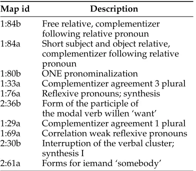
Table 1 lists the 10 variables with the highest HSIC values. Statistical significance at a level of α=0.05 is detected for 65.0% of the linguistic variables using HSIC, 78.3% when using join count analysis, and 52.4% when using the Mantel test. The three methods agree on 99 out of the 143 variables, and HSIC and join count analysis

agree on 118 variables. From manual inspection, it seems that the non-linearity of the geographical patterns may have caused difficulties for the Mantel test. Figure 10 is an example of a variable where HSIC and join count analysis both had an FDR-adjusted p<0.05, but the Mantel test did not detect a significant association.

5.3 Twitter

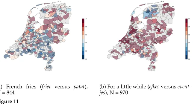
Our Twitter data set consists of 4,039,786 geotagged tweets from the Netherlands, writ-ten between 1 January 2015 and 31 October 2015. We manually selected a set of linguistic variables (Table 2), covering examples of lexical variation (e.g., two different words for referring to french fries), phonological variation (e.g., t-deletion), and syntactic variation (e.g., heb gedaan[‘have done’] vs.gedaan heb [‘done have’]). We are not aware of any previous work on dialectal variation in the Netherlands that uses spatial dependency testing on Twitter data. The number of tweets per municipality varies dramatically, and for the less frequent linguistic variables there are no tweets at all in some municipalities. In our computation of Moran’s I, we only include municipalities with at least one tweet. Table 2 shows the output of each statistical test for this data. Some of these linguistic variables exhibit strong spatial variation, and are identified as statistically significant by all approaches. An example is the different ways of referring to french fries (frietversus patat, Figure 11a), where the figure shows a striking difference between the south and the north of the Netherlands. Another example is Figure 11b, which shows two different ways of saying ‘for a little while’ (efkesversuseventjes). The less common form,efkesis mostly used in Friesland, a province in the north of the Netherlands.

Examples of linguistic variables where the approaches disagree are shown in Figure 12. The first case (Figure 12a) is an example of lexical variation, with two different ways of sayingbyein the Netherlands. A commonly used form isdoei, while houdoeis known to be specific to North-Brabant, a Dutch province in the south of the Netherlands. HSIC and join count analysis both detect a significant pattern, but Moran’s I and the Mantel test do not. The trend is less strong than in the previous

Table 2

Twitter results. The p-values were calculated using 10,000 permutations and corrected for multiple comparisons.

Linguistic variables Description N Moran’s I HSIC Mantel Join counts

Friet / patat french fries 842 0.0004 0.0002 0.0003 0.0003

Proficiat / gefeliciteerd congratulations 14,474 0.0004 0.0002 0.0080 0.0003

Iedereen / een ieder everyone 13,009 0.8542 0.0002 0.8769 0.0432

Doei / aju bye 4,427 0.7163 0.0050 0.2570 0.3868

Efkes / eventjes for a little while 969 0.0036 0.0002 0.0003 0.0003

Naar huis / naar huus to home 3, 942 0.8542 0.1090 0.1245 0.9426

Niet meer / nie meer not anymore 11,596 0.0793 0.0002 0.5590 0.0329

Of niet / of nie or not 1,882 0.8357 0.1010 0.4191 0.9426

-oa- / -ao- e.g.,jaoversusjoa 754 0.0004 0.0002 0.0003 0.0003

Even weer / weer even for a little while again 921 0.0004 0.0002 0.0003 0.0003

Have + participle e.g.,heb gedaan(‘have done’)

vs.gedaan heb(‘done have’)

1,122 0.8587 0.2849 0.6668 0.0255

Be + participle e.g.,ben geweest(‘have been’)

vs.geweest ben(‘been have’)

1,597 0.0793 0.2849 0.7862 0.0051

Spijkerbroek / jeans jeans 1,170 0.7796 0.0002 0.0080 0.0003

Doei/ houdoe bye 4,491 0.5016 0.0002 0.6668 0.0047

(a) French fries (friet versus patat), N = 844

(b) For a little while (efkesversus event-jes), N = 970

Figure 11

Highly significant linguistic variables on Twitter. Gray indicates areas with no data points. The intensity indicates the number of data points.

(a) Bye (doeiversushoudoe), N = 4,491 (b) t-deletion (_{N = 11,596} niet meer vs. nie meer),

Figure 12

Linguistic variables on Twitter where tests disagreed.

examples, but the figure does suggest a higher usage of houdoe in the south of the Netherlands.

Another example is t-deletion for a specific phrase (niet meerversus nie meer), as shown in Figure 12b. Previous dialect research has found that geography is the most important external factor for t-deletion in the Netherlands, with contact zones, such as the Rivers region in the Netherlands (at the intersection of the dialects of the southern province of North-Brabant, the south-west province of Zuid-Holland, and the Veluwe region), having high frequencies of t-deletion (Goeman 1999). Both HSIC and join count analysis report an FDR-adjusted p<0.05, whereas for Moran’s I, the geographical association does not reach the threshold of significance.