Integrating Selectional Constraints and Subcategorization Frames in a Dependency Parser

Subcategorization Frames in a

Dependency Parser

Seyed Abolghasem Mirroshandel

∗

Alexis Nasr

Universit´e Aix-Marseille

Statistical parsers are trained on treebanks that are composed of a few thousand sentences. In order to prevent data sparseness and computational complexity, such parsers make strong inde-pendence hypotheses on the decisions that are made to build a syntactic tree. These indeinde-pendence hypotheses yield a decomposition of the syntactic structures into small pieces, which in turn prevent the parser from adequately modeling many lexico-syntactic phenomena like selectional constraints and subcategorization frames. Additionally, treebanks are several orders of magni-tude too small to observe many lexico-syntactic regularities, such as selectional constraints and subcategorization frames. In this article, we propose a solution to both problems: how to account for patterns that exceed the size of the pieces that are modeled in the parser and how to obtain subcategorization frames and selectional constraints from raw corpora and incorporate them in the parsing process. The method proposed was evaluated on French and on English. The experiments on French showed a decrease of41.6% of selectional constraint violations and a decrease of22%of erroneous subcategorization frame assignment. These figures are lower for English:16.21%in the first case and8.83%in the second.

1. Introduction

The fundamental problem we address in this article was formulated by Joshi (1985) as the following question:How much context-sensitivity is required to provide reasonable structural descriptions?His answer to this question was the extended domain of locality principle of Tree Adjoining Grammars, which allows us to represent in a single structure (an elementary tree1) a predicate and its arguments.

∗Computer Engineering Department, Faculty of Engineering, University of Guilan, Rasht, Iran. E-mail:[email protected].

∗∗Laboratoire d’Informatique Fondamentale, CNRS - Universit´e Aix-Marseille, France. E-mail:[email protected].

1 In the remainder of this article, we will refer to the elementary object manipulated by the parser as

factors, borrowing this term from graph-based parsing.

Submission received: 10 September 2014; revised version received: 3 August 2015; accepted for publication: 28 September 2015.

Context sensitivity and the correct size of domain of locality for a reasonable struc-tural description has always been a major issue for syntactic formalisms and parsers. Giving an overview of the different solutions that have been proposed to answer this question is clearly beyond the scope of this article. We will limit our discussion to the framework of graph-based dependency parsing (Eisner 1996; McDonald and Pereira 2006), in which our study takes place. The basic first-order model makes an extreme choice with respect to the domain of locality by limiting it to one dependency (the score of a tree is the sum of the scores of its dependencies). Second-order models slightly extend the factor sizes to second-order patterns that include a dependency adjacent to the target dependency. It has been shown experimentally that second-order models perform better than first-order ones, which tends to prove that second-order factors do capture important syntactic regularities. More recently, Koo and Collins (2010) proposed extending factor size to three dependencies and showed that such models yield better accuracy than second-order models on the same data. However, extending the order of the models has a high computational cost because the number of factors to be considered in a sentence grows exponentially with the order of the model. Using such models in a Dynamic Programming framework, such as Eisner (1996), becomes quickly intractable in terms of processing time and memory requirements. Additionally, by reliably estimating the scores of such factors we are quickly confronted with the problem of data sparseness.

One can also note that high-order factors are not needed for all syntactic phenom-ena. In fact, most syntactic attachments can be accurately described with first- and second-order models. This is why first- and second-order models perform quite well: They reach a labeled accuracy score of 85.36% and 88.88% for first- and second-order models, respectively, on the French Treebank (Abeill´e, Cl´ement, and Toussenel 2003). The same models trained on the Penn Treebank (Marcus, Marcinkiewicz, and Santorini 1993) reach 88.57% and 91.76% labeled accuracy score, respectively. The extension of the domain of locality can therefore be limited to some syntactic phenomena. This is the case in Tree Adjoining Grammars for which the extended domain of locality only concerned some aspects of syntax, namely, subcategorization.

The solution we explore in this article, in order to take high-order factors into account in a parser, is to decompose the parsing process into two sub-processes. One of them is in charge of local syntactic phenomena and does not need a high-order model and the other takes care of syntactic phenomena that are beyond the scope of the first one. We will call the first one parsing and the second one patch-ing. The patching process is responsible for modeling two important aspects of syntax, Selectional Constraints (SCs) and Subcategorization Frames (SFs), which are usually poorly modeled in parsers, as we will show in Sections 7 and 8. Parsing and patching differ in two important aspects. First, they rely on different search algorithms. The first one is based on Dynamic Programming and the other one uses Integer Linear Programming (ILP). Second, they rely on different data sets. The first uses a standard treebank whereas the second uses much larger unannotated corpora.

The second difference between parsing and patching is the data sets that were used to train them. The parser is trained on a standard treebank whereas the patching model is trained on a raw corpus that is several orders of magnitude larger. The reason for this difference comes from the fact that high-order factors used to model SFs and SCs contain up to three lexical elements and cannot be accurately modeled using available treebanks. It has been shown by Gildea (2001) and Bikel (2004) that bilexical dependencies of the Collins parser (Collins 1997) have a very limited impact on the performances of the parser, although they were supposed to play a key role for some important ambiguous syntactic attachments. The reason for this is that treebanks are not large enough to correctly model bilexical dependencies. We show in Sections 7.2 and 8.2 that current treebanks are much too limited in size to accurately model SCs and SFs.

Other solutions have been proposed in the literature in order to combine local and global syntactic phenomena in a parser. Parse reranking is one of them. The idea is to produce then-best parses for a sentence and rerank them using higher order features, such as in Collins and Koo (2005) and Charniak and Johnson (2005). This solution has the advantage of drastically limiting the search space of the high-order search algorithm to thekbest parses. Although the parsing architecture we propose in this article does usek-best parse lists, our solution allows us to combine dependencies that appear in any of the parses of the list. We show in Section 6.3 that combining dependencies that appear in any parse of ak-best list can yield parses that are more accurate than the best parse of thisk-best list. Our method is closer to forest rescoring (Huang and Chiang 2007) or forest reranking (Huang 2008).

Another solution to combine local and global decisions is to represent the local and the global constraints as a single ILP program. This solution is possible because dependency parsing can be framed as an ILP program. Riedel and Clarke (2006) propose a formulation of nonprojective dependency parsing as an ILP program. This program, however, requires an exponential number of variables. Martins, Smith, and Xing (2009) propose a more concise formulation that only requires a polynomial number of variables and constraints. Martins, Almeida, and Smith (2013) propose extending the model to third-order factors and using dual decomposition. All these approaches have in common their ability to produce nonprojective structures (Lecerf 1961). Our work departs from these approaches in that it uses a dynamic programming parser combined with an ILP solver. Additionally, we do not take nonprojective structures into account.

The structure of this article is as follows. In Section 2 we describe the type of parser used in this work. Section 3 describes the patching process that detects, in a given sentence, a set of optimal SFs and SCs, using ILP. The exact nature of SFs and SCs is described in that section. Section 4 proposes a way to combine the solutions produced by the two methods using constrained parsing. In Section 5, we justify the use of ILP by showing that the patching process is actually NP-complete. Sections 6, 7, and 8 constitute the experimental part of this work. Section 6 describes the experimental set-up, and Sections 7 and 8, respectively, give results obtained on French and English. Section 9 concludes the article.

and could not treat the two problems jointly. Additionally, we extended the experimen-tal part of our work to English, whereas previous work only concerned French.

2. Parsing

In this section, we briefly present the graph-based approach for projective dependency parsing. We then introduce an extension to this kind of parser, which we call con-strained parsing, that forces the parser to include some specific patterns in its output. Then, a simple confidence measure that indicates how confident the parser is about any subpart of the solution is presented.

2.1 Graph-Based Parsing

Graph-based parsing (McDonald, Crammer, and Pereira 2005a; K ¨ubler, McDonald, and Nivre 2009) defines a framework for parsing that does not make use of a generative grammar. In such a framework, given a sentence S=w1. . .wl, any dependency tree2 for S is a possible syntactic structure forS. The heart of a graph-based parser is the scoring function, which assigns a scores(T) to every treeT∈T(S), whereT(S) denotes the set of all dependency trees of sentence S. Such scores are usually the sum of the scores of subparts ofS. The parser returns the tree that maximizes such a score:

ˆ

T=arg max T∈T(S)

X

ψ∈ψ(T)

s(ψ) (1)

In Equation (1), ψ(T) is the set of all the relevant subparts of tree T and s(ψ) is the score of subpartψ. The scores of the subparts are computed using machine learning algorithms on a treebank, such as McDonald, Crammer, and Pereira (2005b).

As already mentioned in Section 1, several decompositions of the tree into sub-parts are possible and yield models of increasing complexity. The most simple one is the first-order model, which simply decomposes a tree into single dependencies and assigns a score to a dependency, irrespective of its context. The more popular model is thesecond-order model, which decomposes a tree into subparts made of two dependencies.

Solving Equation (1) cannot be done naively for combinatorial reasons: The setT(S) contains an exponential number of trees. However, it can be solved in polynomial time using dynamic programming (Eisner 2000).

2.2 Constrained Parsing

The graph-based framework allows us to impose structural constraints on the parses that are produced by the parser in a straightforward way, a feature that will prove to be valuable in this work.

A sentence S=w1. . .wl is a parser with a scoring functions and a dependency

d=(i,r,j), such thatiis the position of the governor,jthe position of the dependent,

2 A dependency tree for sentenceS=w1. . .wland the dependency relation setRis a directed labeled tree

andrthe dependency label, with 1≤i,j≤l. We can define a new scoring functions+_d in the following way:

s+_d (i0,r0,j0)=

 



−∞ ifj0=jand (i06=iorr06=r) s(i0,r0,j0) otherwise

When running the parser on sentenceS, with the scoring functions+_d, one can be sure that dependencydwill be part of the solution produced by the parser because the score of all its competing dependencies (i.e., dependencies of the form (i0,r0,j0) with different governors (i06=i) or labels (r06=r) and the same dependent (j0=j)) are set to−∞. As a result, the overall score of trees that have such competing dependencies cannot be higher than the trees that have our desired dependency. In other words, the resulting parse tree will contain dependencyd. This feature will be used in Section 4 in order to parse a sentence for which a certain number of dependencies are set in advance.

Functions+_d can be extended in order to force the presence of any set of dependen-cies in the output of the parser. SupposeDis a set of dependencies; we then defines+D

the following way:

s+_D(i,r,j)=

 



s+_d (i,r,j) if∃d∈Dsuch thatd=(·,·,j)

s(i,r,j) otherwise

Modifying the scoring function of the parser to force the inclusion or the ex-clusion of some dependencies has already been used in the literature. It was used by Koo and Collins (2010) to ignore dependencies whose probability was below a certain threshold and by Rush and Petrov (2012) in their multi-pass, coarse-to-fine approach.

2.3 Confidence Measure

The other extension of graph-based parsers that we use in this work is the computation of confidence measures on the output of the parser. The confidence measure used is based on the estimation of posterior probability of a subtree, computed on thek-best list of parses of a sentence. It is very close to confidence measures used for speech recog-nition (Wessel et al. 2001) and differs from confidence measures used for parsing, such as S´anchez-S´aez, S´anchez, and Bened´ı (2009) or Hwa (2004), which compute confidence measures for complete parses of a sentence.

Given the k-best parses of a sentence and a subtree ∆ present in at least one of the k-best parses, let C(∆) be the number of occurrences of ∆ in the k-best parse set. Then CM(∆), the confidence measure associated with ∆, is computed as:

Mirroshandel and Nasr (2011) and Mirroshandel, Nasr, and Roux (2012) provide more detail on the performance of this measure. Other confidence measures could be used, such as the edge expectation described in McDonald and Satta (2007), or inside-outside probabilities.

3. Patching

In this section, we introduce the process of patching a sentence. The general idea of patching sentence S is to detect in S the occurrences of predefined configurations. In section 3.1 we introduce Lexico-Syntactic Configurations, which correspond to the patches. We describe in section 3.2 the process of selecting an optimal set of patches on a sentence (finding an optimal solution is not trivial since patches have scores and some patches are incompatible). Sections 3.3 and 3.4, respectively, describe two instances of the patching problem, namely, subcategorization frame selection and se-lectional constraint satisfaction. Section 3.5 shows how both problems can be solved together.

3.1 Lexico-Syntactic Configuration

A Lexico-syntactic Configuration (LSC) is a pair (s,T) where s is a numerical value, called thescoreof the LSC, andTis a dependency tree of arbitrary size. Every node of the dependency tree has five features: a syntactic function, a part of speech, a lemma, a fledged form, and an index, which represents a position in a sentence. The features of every node can either be specified or left unspecified. Given an LSCi,s(i) will represent the score ofiandT(i) will represent its tree.

Index features are always unspecified in an LSC. What follows is an example of an LSC that corresponds to the sentenceJean offre des fleurs `a N[Jean offers flowers to N]. The five features of the dependency tree nodes are represented between square brackets and are separated by colons.

(0.028, [:V:offrir:offre:]( [SUJ:N:Jean:Jean:], [OBJ:N:fleur:fleurs:], [A-OBJ:P:a:a:](

[OBJ:N:::])))

An instantiated LSC (ILSC) is an LSC such that all its node features (in particular, index features) are specified. We will noteR(i) as the index of the root of ILSCiandL(i) as the set of its leaf indices.

Given the sentenceJean offre des fleurs `a Marieand the LSC, the instantiation of the LSC on the sentence gives the following ILSC:

(0.028, [:V:offrir:offre:2]( [SUJ:N:Jean:Jean:1], [OBJ:N:fleur:fleurs:4], [A-OBJ:P:a:a:5](

3.2 Selecting the Optimal Set of ILSCs

Given a sentenceS, and a setLof LSCs, we define the setIof all possible instantiations of elements ofLonS. Once the setI has been defined, our aim is to select a subset ˆI

made of compatible3ILSCs such that

ˆ

I=arg max I⊆I

X

C∈I

s(C) (2)

As it was the case for Equation (1), Equation (2) cannot be solved naively for combinatorial reasons: The power-set ofIcontains an exponential number of elements. Such a problem will be solved using ILP.

In order to solve Equation (2), the setI of all possible instantiations of the LSCs of setLfor a given sentenceSmust be built. Several methods can be used to compute such a set, as described in Section 6.3.

We will see in Sections 3.3 and 3.4 two instances of the patching problem. In Section 3.3, ILSCs will represent SFs, and in Section 3.4, they will represent SCs.

3.3 Subcategorization Frames

A subcategorization frame is a special kind of LSC. Its root is a predicate and its leaves are the arguments of the predicate.

Here is an example of an SF for the French verbdonner[to give]. It is a ditransitive frame; it has both a direct object and an indirect one introduced by the preposition`aas inJean donne un livre `a Marie.[Jean gives a book toMarie].

(0.028, [:V:donner::] ( [SUJ:N:::], [OBJ:N:::], [A-OBJ:P:a:a:] (

[OBJ:N:::])))

The score of an SFT must reflect the tendency of a verbV (the root of the SF) to select the given SF. This scoresSFis simply the conditional probabilityP(T|V) estimated data sets that will be described in Sections 7 and 8.

3.3.1 Selecting the Optimal Set of Subcategorization Frames.Given a sentence Sof length Nand the set I of Instantiated Subcategorization Frames (ISFs) overS, the selection of the optimal set ˆI⊆I is done by solving the general equation 2, using ILP, with constraints that are specific to SF selection. The exact formulation of the ILP program is now described.

r

– αj_i=1 if word numberiis the predicate of ISF numberj, andαj_i=0 otherwise.

– βj_i=1 if word numberiis an argument of ISF numberj, andβj_i=0 otherwise.

Variablesαj_iandβj_iare not defined for all values ofiandj. A variableαj_iis defined only if wordican be the predicate of ISFj∈I.

r

– a word is the predicate of at most one ISF:

∀i∈ {1,. . .,N} X j∈I

αj_i≤1

– a word cannot be an argument of more than one ISF:

∀i∈ {1,. . .,N} X j∈I

βj_i≤1

– for an ISF to be selected, both its predicate and all its arguments (i.e.,L(j)) must be selected:

∀j∈ {1,. . .,|I|} |L(j)|αj_R(j)− X l∈L(j)

βj_l=0

r

maxX

j∈I

αj_R(j)sSF(j)

Let us illustrate this process on the sentenceJean rend le livre qu’il a emprunt´e `a la biblioth`eque.[Jean returns the book that he has borrowed from the library.] which contains an ambiguous prepositional phrase attachment: the prepositional phrase `a la biblioth`eque [from the library] can be attached either to the verbrendre[return] or to the verbemprunter [borrow] . The setIis composed of the four following ISFs:

1 (0.2,[:V:rend:rendre:2]( [SUJ:N:Jean:Jean:1], [OBJ:N:livre:livre:4]))

2 (0.4,[:V:rend:rendre:2]( [SUJ:N:Jean:Jean:1], [OBJ:N:livre:livre:4], [A-OBJ:P:a:a:9](

[OBJ:N:biblio.:biblio.:11])))

3 (0.3,[:V:emprunte:emprunter:8] ( [SUJ:N:il:il:6],

[OBJ:N:qu’:que:5]))

4 (0.6,[:V:emprunte:emprunter:8] ( [SUJ:N:il:il:6],

[OBJ:N:qu’:que:5], [A-OBJ:P:a:a:9] (

The actual ILP program is the following:

r

α1₂,α2₂ verbrendrecan select ISF 1 or 2 α3₈,α4₈ verbempruntercan select ISF 3 or 4 β1₁,β2₁ nounJeancan be the subject of ISF 1 or 2 β1

4,β24 nounlivrecan be the object of ISF 1 or 2

β1₁₁ nounbibliothequecan be the indirect object of ISF 2 β3₅,β4₅ relative pronounquecan be the object of ISF 3 or 4 β3₆,β4₆ pronounilcan be the subject of ISF 3 or 4

β4₁₁ nounbibliothequecan be the indirect object of ISF 4

r

– a word is the predicate of at most one ISF:

α1₂+α2₂≤1 verbrendrecannot be the predicate of both ISF 1 and 2 α3₈+α4₈≤1 verbempruntercannot be the predicate of both ISF 3 and 4

– a word cannot be an argument of more than one ISF:

β1₁+β2₁ ≤1 NounJeancannot be the subject of both ISF 1 and 2 β1₄+β2₄ ≤1 Nounlivrecannot be the object of both ISF 1 and 2 β3₅+β4₅ ≤1 Relative pronounquecannot be the object of

both ISF 3 and 4 β3

6+β46 ≤1 Pronounilcannot be the subject of both ISF 3 and 4 β2₁₁+β4₁₁≤1 Nounbibliothequecannot be the object of both ISF 2 and 4

– for an ISF to be selected, both its predicate and all its arguments must be selected:

2α1₂−(β₁1+β1₄)=0 ISF 1 must have a subject and an object 3α2₂−(β2₁+β2₄+β2₁₁)=0 ISF 2 must have a subject, an object and an

indirect object

2α3₈−(β₅3+β3₆)=0 ISF 3 must have a subject and an object 3α4₈−(β4₅+β4₆+β4₁₁)=0 ISF 4 must have a subject, an object and an

indirect object

r

max(0.2α1₂+0.4α2₂+0.3α3₈+0.6α4₈)

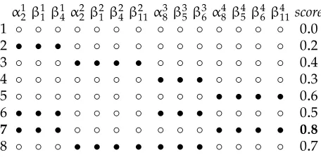
The problem admits eight solutions, represented in Figure 1. Each column corresponds to a variable. Black dots (•) correspond to the value 1 and white dots (◦) to the value 0. The optimal solution is solution number 7 for which verbrendreselects ISF 1 and verbemprunter selects ISF 4. In this solution, the prepositional phrase `a la biblioth`equeis attached to the verbrendre.

3.4 Selectional Constraints

α1₂β1₁ β1₄ α2₂ β2₁β2₄β2₁₁ α3₈β3₅ β3₆ α₈4 β4₅β4₆β4₁₁ score 1 ◦ ◦ ◦ ◦ ◦ ◦ ◦ ◦ ◦ ◦ ◦ ◦ ◦ ◦ 0.0 2 • • • ◦ ◦ ◦ ◦ ◦ ◦ ◦ ◦ ◦ ◦ ◦ 0.2 3 ◦ ◦ ◦ • • • • ◦ ◦ ◦ ◦ ◦ ◦ ◦ 0.4 4 ◦ ◦ ◦ ◦ ◦ ◦ ◦ • • • ◦ ◦ ◦ ◦ 0.3 5 ◦ ◦ ◦ ◦ ◦ ◦ ◦ ◦ ◦ ◦ • • • • 0.6 6 • • • ◦ ◦ ◦ ◦ • • • ◦ ◦ ◦ ◦ 0.5 7 • • • ◦ ◦ ◦ ◦ ◦ ◦ ◦ • • • • 0.8 8 ◦ ◦ ◦ • • • • • • • ◦ ◦ ◦ ◦ 0.7 Figure 1

Representation of the eight solutions to the ILP problem.

A set of four SC patterns, described here, have been defined. The first two describe a subject and object selectional constraint, respectively. Patterns 3 and 4, respectively, describe selectional constraints on an indirect object introduced by the prepositionde and`a:

([:V:::]([SUJ:N:::])) ([:V:::]([OBJ:N:::]))

([:V:::]([DE-OBJ:P:de::]([OBJ:N:::]))) ([:V:::]([A-OBJ:P:a::]([OBJ:N:::])))

Three important formal features distinguish SFs and SCs:

r

r

in a specific syntactic configuration) whereas SFs model unilexical phenomena (the tendency of one word to select a specific SF).

r

Note that SC patterns are described at a surface syntactic level and, in the case of control and raising verbs, the SC pattern will be defined over the subject and the control/raising verb and not the embedded verb—although the selectional constraint is between the subject and the embedded verb. In the event of coordination of subject or object, only one of the coordinated elements will be extracted.

The score of an SC should reflect the tendency of the root lemma lr and the leaf lemmallto appear together in configurationC. It should be maximal if wheneverlr oc-curs as the root of configurationC, the leaf position is occupied bylland, symmetrically, if wheneverlloccurs as the leaf of configurationC, the root position is occupied bylr. A function that conforms to such a behavior is the following:

sSC(C,lr,ll)= 1₂

C(C,lr,ll)

C(C,lr,∗)

+C(C,lr,ll)

C(C,∗,ll)

This function takes its values between 0 (lr andll never co-occur) and 1 (lr andll always co-occur). It is close to pointwise mutual information (Church and Hanks 1990) but takes its values between 0 and 1.

3.4.1 Selecting the Optimal Set of Selectional Constraints.Given a sentenceSof lengthN and the setI0of Instantiated Selectional Constraints (ISCs) overS, the selection of the optimal set ˆI0_⊆I0_{is framed as the following ILP program.}

r

– γj_i=1 if word numberiis the root of ISC numberj, andγj_i=0 otherwise.

– δj_iif word numberiis the leaf of ISC numberj, andδj_i=0 otherwise.

r

– a word cannot be the leaf of more than one ISC

∀i∈ {1,. . .N} X j∈I0

δj_i≤1

– for an ISCjto be selected, both its root (i.e.,R(j)) and its leaf must be selected

∀j∈ {1,. . .,|I0|}γj_R(j)−δj_d∈L(j)=0

r

maxX

j∈I0

γj_R(j)sSC(j)

Let us illustrate the selection process on the same sentence (Jean rend le livre qu’il a emprunt´e `a la biblioth`eque.). A set of four ISCs is defined:

5 (0.2,[:V:rend:rendre:2] ([SUJ:N:Jean:Jean:1])) 6 (0.2,[:V:rend:rendre:2]

([OBJ:N:livre:livre:4])) 7 (0.4,[:V:rend:rendre:2]

([A-OBJ:P:a:a:9]

([OBJ:N:biblio.:biblio.:11]))) 8 (0.6,[:V:emprunte:emprunter:8]

([A-OBJ:P:a:a:9]

([OBJ:N:biblio.:biblio.:11])))

The actual IL program is the following:

r

γ5₂,γ6₂,γ7₂ verbrendrecan be the root of ISC 5, 6, and 7 γ8₈ verbempruntercan be the root of ISC 8 δ5₁ nounJeancan be the leaf of ISC 5 δ6₄ nounlivrecan be the leaf of ISC 6 δ7

r

– a word cannot be the leaf of more than one ISC

δ5₁≤1 nounJeancan only be the leaf of ISC 5 δ6

4≤1 nounlivrecan only be the leaf of ISC 6

δ7₁₁+δ8₁₁≤1 nounbiblioth`equecannot be the leaf of both ISC 7 and 8

– for an ISC to be selected, both its root and its leaf must be selected γ5₂−δ5₁=0 ISC 5 must have a root and a leaf

γ6₂−δ6₄=0 ISC 6 must have a root and a leaf γ7₂−δ7₁₁=0 ISC 7 must have a root and a leaf γ8₈−δ8₁₁=0 ISC 8 must have a root and a leaf

r

max(0.2γ5₂+0.2γ6₂+0.4γ7₂+0.6γ8₈)

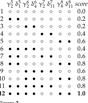
The problem admits twelve solutions, represented in Figure 2. The optimal solution is solution number 12, in which the prepositional phrase`a la biblioth`equeis attached to the verbemprunter.

3.5 Combining Subcategorization Frames and Selectional Constraints

SF selection and SC satisfaction can be combined together in a single ILP program that combines the variables and constraints of the two problems and adds a new constraint that takes care of the incompatibilities of SCs and SFs.

Given a sentenceSof lengthN, the setIof ISFs and the setI0_{of ISCs, the selection} of the optimal set ˆI00_⊆I∪I0_{is the solution of the following program:}

r

αj_i,βj_i,γj_i,δj_i

r

– All the constraints of ISF selection and ISC satisfaction.

γ5₂ δ5₁γ6₂δ6₄ γ7₂ δ7₁₁γ8₈δ8₁₁score 1 ◦ ◦ ◦ ◦ ◦ ◦ ◦ ◦ 0.0 2 • • ◦ ◦ ◦ ◦ ◦ ◦ 0.2 3 ◦ ◦ • • ◦ ◦ ◦ ◦ 0.2 4 ◦ ◦ ◦ ◦ • • ◦ ◦ 0.4 5 ◦ ◦ ◦ ◦ ◦ ◦ • • 0.6 6 • • • • ◦ ◦ ◦ ◦ 0.4 7 • • ◦ ◦ • • ◦ ◦ 0.6 8 • • ◦ ◦ ◦ ◦ • • 0.8 9 ◦ ◦ • • • • ◦ ◦ 0.6 10 ◦ ◦ • • ◦ ◦ • • 0.8 11 • • • • • • ◦ ◦ 0.8 12 • • • • ◦ ◦ • • 1.0 Figure 2

– Incompatible ISFs and ISCs cannot be selected together.

An ISFjand an ISCj0are not compatible if they share a common leaf (i0) but have different roots (i6=i00). Such a constraint can be modeled by the following inequality:

∀i,i0,i00,j,j0s.t.i6=i00, 2αj_i+βj_i0+2γ

j0

i00 +δ

j0

i06=5

r

max



 X

j∈I0

δj_R(j)sSC(j)+

X

j∈I

αj_R(j)sSF(j)





The actual ILP program is too large and redundant with the two preceding ones to be exposed fully here. Its set of variables and constraints is the union of the variables and the constraints of the preceding ones, plus the two following ones:

2α2

2+β211+2γ88+δ8116=5 ISF 2 and ISC 8 are incompatible 2α4₈+β4₁₁+2γ7₂+δ7₁₁6=5 ISF 4 and ISC 7 are incompatible

Definition of the objective function:

max(0.2γ5₂+0.2γ6₂+0.4γ7₂+0.6γ8₈+0.2α1₂+0.4α2₂+0.3α3₈+0.6α4₈)

The problem admits 94 solutions. The optimal solution is made of ISFs 1 and 4, and ISCs 5, 6, and 8.

4. Combining Parsing and Patching

Two processes have been described in Sections 2 and 3. In the first one, parsing is based on dynamic programming and produces a complete parse of a sentenceS whereas in the second, patching is based on ILP and produces a partial parse ofS: the set ˆI00_made of ISCs and ISFs.

We would like now to produce a parse for sentence S that combines constraints coming from parsing and patching. We have exposed in Section 1 the reasons why we chose to keep these two processes separated and to combine their solutions to produce a single parse. The whole process is composed of three steps:

1. SentenceSis first parsed using a first-order parser and the set ofk-best parses is produced in order to generate the setIof ISFs and the setI0of ISCs.

2. Patching is then performed and computes the optimal set ˆI00_⊆I∪I0_of ISFs and ISCs.

3. A new scoring functions+_ˆ

I00 is then computed and a second-order parser

This setting is strongly biased in favor of the patching process. Because of the nature of the scoring functions+_ˆ

I00, the ISFs and ISCs computed during the patching step are

kept in the final solution even if considered unlikely by the parser. In practice, this solution does not perform well.

In order to let the parser influence the solution of the patching process, the confi-dence measureCM, defined in Section 2, is introduced in the objective function of the ILP. Recall that CM(∆) indicates how confident the parser is about sub-tree ∆. This quantity is added to the scores of SFs and SCs introduced in sections 3.3 and 3.4.

The new scoring functions ˆsSFand ˆsSCare defined as follows:

ˆ

sSF(∆)=(1−µ1)sSF(∆)+µ1CM(∆)

ˆ

sSC(∆)=(1−µ2)sSC(∆)+µ2CM(∆)

where the values ofµ₁andµ₂are determined experimentally on a development set. In the definition of ˆsSF and ˆsSC, the first component (sSF andsSC) can be interpreted as a lexical score and the second one (CM) as a syntactic score.

After patching is performed and the set ˆI00_{is computed, the scoring function of the} second order parser is modified in order to force the ISFs and ISCs of ˆI00_{to appear in} the parser’s solution.

As explained in Section 2.2, the modification of the scoring function modifies only the scores of first-order factors (single dependencies). The modification amounts to setting to −∞the scores of the dependencies that compete with those dependencies that occur in ˆI00_{. At this point, the set ˆI}00 _{is just considered as a set of first-order} factors, whatever the ILSC they are a member of. The scores of second-order factors are not modified. This solution works because the second-order parser uses both first-and order factors. There is no need to modify the scoring function of the second-(or higher) order factors since the first-order factors that they are composed of will be discarded anyway, because of their modified scores.

Let us illustrate the process on the sentenceJean commande une glace `a la serveuse. [Jean orders an ice-cream from the waitress.]. The parser output for this sentence wrongly attaches the preposition`ato the nounglacewhereas it should be attached to the verbcommander. Suppose that, after patching, the set ˆI00_{is made of the ISF (commander,} SBJ:N OBJ:N AOBJ:N): the verbcommandertakes an indirect object introduced by prepo-sition`a, and the ISC (VaN, commander, serveuse): the nounserveuseis the indirect object of the verbcommander. At this point ˆI00<sub>is viewed as the set of dependencies{(commande,</sub> SUJ, Jean), (commande, OBJ, glace), (commande, AOBJ, `a), (`a, OBJ, serveuse)}. The score of all competing dependencies, which are all dependencies that have eitherJean,glace,`a, or serveuseas a dependent, are set to−∞and will be discarded from the parser solution.

5. Complexity of the Patching Problem

Could patching be solved using a polynomial algorithm? How does a general ILP solver perform, in practice, on our data?

We will answer these questions in two steps. First, we will prove in this section that patching is actually NP-complete. Building the optimal solution requires exponential time in the worst case. Second, we will show in Section 7, that, due to the size of the instances at hand, the processing time using a general ILP solver is reasonable.

In order to prove that patching is NP-complete, we will first show that some instances of patching can be expressed as a Set Packing problem (SP), known to be NP-complete (Karp 1972). The representation of a patching problem as a SP problem will be called patching as a Set Packing problem (P-SP). We will then reduce SP to P-SP by showing that any instance of SP can be represented as an instance of P-SP, which will prove the NP-completeness of P-SP and therefore the NP-completeness of patching.

The Set Packing decision problem is the following: Given a finite setSand a listUof subsets ofS, are thereksubsets inUthat are pairwise disjoint? The optimization version of SP, the Maximum Set Packing problem (MSP), looks for the maximum number of pairwise disjoint sets inU.

We will show that a subset of the instances of patching can be expressed as an MSP. More precisely, we restrict ourselves to instances such that:

r

r

The reason why we limit ourselves to a subset of patching is that our goal is to reduce any SP problem to a patching problem. Reducing an SP problem to some special cases of patching is enough to prove NP-completeness of patching. Patching in the general case might be represented as an MSP problem but this is not our goal.

Recall that patching with ISF is subject to three constraints:

C1: a word cannot be the predicate of more than one ISF C2: a word cannot be the argument of more than one ISF

C3: for an ISF to be selected, both its predicate and its arguments must be selected

Given a sentenceS=w1,. . .,wnand a setIof ISFs onS, let us associate withSthe setS={1,. . .,n}. As a first approximation, let us represent an ISF ofI as the subset ofS composed of the indices of the arguments of the ISF. The list of ISFI is therefore represented as a listU of subsets ofS. Solving the MSP problem for (S,U) produces the optimal solution ˆU that satisfiesC2 and partlyC3.C2 is satisfied because the elements of ˆU are pairwise disjoint.C3is partly satisfied because all the arguments of an ISF are selected altogether, but not the predicate.

having word wp as a predicate and wordswa1. . .wak as arguments is represented as

the subset{a1,. . .ak,p+n}. The solution to the MSP problem using this representation clearly verifies our three constraints.

Given a sentence S=w1,. . .,wn and a set of ISFs I, we can build the set S= {1,. . .,N}, withN≥2n4 and the listU such that any element ofU corresponds to an ISF ofI, using the method described here. The solution to the MSP on input (S,U) is equivalent to the solution of patching on input (S,I). Such an MSP problem will be called a P-MSP problem (patching as Maximum Set Packing). Recall that the decision version of the problem is called P-SP (patching as Set Packing).

In order to prove the NP-completeness of patching, we will reduce any instance of SP to an instance of P-SP. Given the setS ={1,. . .,n}and the listU =(U₁,. . .,U_m) of subsets ofS, let us build the setS0={1,. . .,n+m}and the list U0=(U₁0,. . .,U_m0) such that U_i0=U_i∪ {i+n}. The pair (S0,U0) is a valid instance of P-SP. The solution of P-SP on input (S0,U0) corresponds to the solution of SP on input (S,U).5 _{If there} was a polynomial algorithm to solve patching, there would be a polynomial algorithm to solve SP. SP would therefore not be NP-complete, which is incorrect. Patching is therefore NP-complete.

6. Experimental Set-up

We describe in this section and the two following ones the experimental part of this work. This section concerns language-independent aspects of the experimental set-up and Sections 7 and 8 describe the experiments and results obtained, respectively, on French and English data.

The complete experiments involve two offline and three online processes. The offline processes are:

1. Training the parser on a treebank.

2. Extracting SFs and SCs from raw data and computing their scores. The result of this process is the setL.

The online processes are:

1. Generating the setIof ISFs and ISCs on a sentenceS, usingL. We will call this processcandidate generation.

2. Patching sentenceSwithI, using ILP. The result of this process is the set ˆI. 3. ParsingSunder the constraints defined by ˆI.

The remaining part of this section is organized as follows: Section 6.1 gives some details about the parser that we use; Section 6.2 describes some aspects of the extraction of SCs and SFs from raw data. Section 6.3 focuses on the candidate generation process.

4 At this point, we can impose thatN=2n. We will need the conditionN≥2nlater in order to prove the reducibility of SP to P-SP. The conditionN≥2nis not harmful, ifN>2n, the range [2n+1,. . .,N] will simply not be used when representing a patching instance as a P-SP instance.

5 It is important to note that in the setU_i0=Ui∪ {i+n}, adding the new elementi+ndoes not introduce

any new constraint because this element only occurs in the setU_i0and will not conflict with any element of another setU0

We have decided not to devote specific sections to the processes of patching and parsing under constraints. Patching has been described in full in Section 3. The ILP solver we have used is SCIP (Achterberg 2009). Parsing under constraints has been described in section 2.2.

6.1 Parser

The parser used for our experiments is the second-order graph-based parser implemen-tation of Bohnet (2010). We have extended the decoding part of the parser in order to implement constrained parsing andk-best parses generation. The first-order extension is based on algorithm 3 of Huang and Chiang (2005), and the second-order extension relies on a non-optimal greedy search algorithm.

The parser uses the 101 feature templates, described in Table 4 of Bohnet (2010). Each feature template describes the governor and dependent of a labeled dependency, called the target dependency, as well as some features of its neighborhood. Every feature is associated with a score, computed on a treebank. A parse tree score is defined as the sum of the features it contains and the parser looks for the parse tree with the highest score.

Feature templates are divided into six sets:

Standard Feature Templates are the standard first-order feature templates. They de-scribe the governor and the dependent of the target dependency. The governor and the dependent are described by combinations of their part of speech, lemma, morphological features, and fledged form.

Linear Feature Templates describe the immediate linear neighbors of the governor and/or the dependent of the target dependency. In such templates, governor, dependent, and neighbors are represented by their part of speech.

Grandchild Feature Templates are the first type of second-order features. They de-scribe the structural neighborhood of the target dependency. This neighborhood is limited to a child of the dependent of the target dependency. Such templates are suited to model linguistic phenomena such as prepositional attachments.

Linear Grandchild Feature Templates describe the immediate linear neighbors of the governor, the dependent, and the grandchild of the target dependency.

Sibling Feature Templates are the second type of second-order feature templates. They describe the structural neighborhood of the target dependency limited to a sibling of the dependent of the target dependency. Such templates are suited, for example, to prevent the repetition of non-repeatable dependencies.

Linear Sibling Feature Templates describe the immediate linear neighbors of the governor, and the two siblings.

When run in first-order mode, the parser only uses Standard and Linear features. All features are used when the parser is run in second-order mode.

Four measures are used to evaluate the parser. The first two are standard whereas the third and fourth have been specifically defined to monitor the effect of our model on the performances of the parser:

Unlabeled Accuracy Score (UAS) of a treeTis the ratio of correct unlabeled dependen-cies inT.

Subcategorization Frame Accuracy Score (SFAS) of a tree Tis the ratio of verbs in T that have been assigned their correct subcategorization frame. More precisely, given the reference parseRfor sentenceSand the outputHof the parser for the same sentence, all ISFs are extracted fromRandH, yielding the two setsRSFand

HSF. SFAS is the recall ofHSFwith respect toRSF(|RSF|R∩SFH|SF|).

Selectional Constraint Accuracy Score (SCAS) of a treeTis the ratio of correct occur-rences of SC patterns inT. More precisely, given a gold standard treeRfor sentence Sand the outputHof the parser for the same sentence, all ISCs are extracted from RandH, yielding the two setsRSCandHSC. SCAS is the recall ofHSCwith respect toRSC.

6.2 Extracting SFs and SCs from Raw Data

The LSC extraction process takes as input raw data and produces a set Lcomposed of SCs and SFs. The process is straightforward: The corpora are first parsed, then LSC templates are applied on the parses, using unification, in order to produce SCs and SFs along with their number of occurrences. These numbers are used to compute selectional constraints scores (sSC), as defined in Section 3.4, and subcategorization frame scores (sSF) as described in Section 3.3.

The extraction of lexical co-occurrences from raw data has been a very active direc-tion of research for many years. Giving an exhaustive descripdirec-tion of this body of work is clearly beyond the aim of this article. The dominant approach for extracting lexical co-occurrences, as described, for example, in Volk (2001), Nakov and Hearst (2005), Pitler et al. (2010), and Zhou et al. (2011) directly model word co-occurrences on word strings. Co-occurrences of pairs of words are first collected on raw corpora orn-grams. Based on the counts produced, lexical affinity scores are computed. The detection of pairs of word co-occurrences is generally very simple: It is either based on the direct adjacency of the words in the string or their co-occurrence in a window of a few words. Bansal and Klein (2011) and Nakov and Hearst (2005) rely on the same sort of techniques but use more sophisticated patterns, based on simple paraphrase rules, for identifying co-occurrences. Our work departs from these approaches by extracting co-occurences in specific lexicosyntactic contexts that correspond to our SC patterns. Our approach allows us to extract more fine-grained phenomena but, being based on automatically parsed data, it is more error-prone.

Extracting SFs for verbs from raw data has also been an active direction of research for a long time, dating back at least to the work of Brent (1991) and Manning (1993). More recently, Messiant et al. (2008) proposed such a system for French verbs. The method we use for extracting SF is not novel with respect to such work. Our aim was not to devise new extraction techniques, but merely to evaluate the resource produced by such techniques for statistical parsing.

6.3 Candidate Generation

process is very important because it defines the search space of the patching process. If the search space is not wide enough, it might fail to contain the correct solution. If it is too wide, the IL programs generated will be too large to be solved in a reasonable amount of time.

Several methods can be used in order to perform the candidate generation process. One could computeI on the linear representation ofS enriched with part of speech tags and lemmas. Bechet and Nasr (2009), for example, represent LSCs as finite-state automata that are matched on S. This method has a tendency to over-generate and proposes some very unlikely instantiations.

In order to constrain the instantiation process, some syntax can be used. For exam-ple, LSCs can be matched on a setT of possible parses ofSin order to produceI. The setT itself can be thek-best parses produced by a parser, as in parse reranking (Collins and Koo 2005; Charniak and Johnson 2005). It can also be built using parse correction techniques (Hall and Nov´ak 2005; Attardi and Ciaramita 2007; Henestroza and Candito 2011). In the latter approach, a parse treeTofSis first built, using a parser, and parse cor-rection rules are applied on it in order to build other parses that might correct errors ofT. The solution that we propose uses a parser to produce a listT ={T1,. . .,Tk}ofk -best parses, such as in parse reranking. But this list is merged into a set of dependencies

D_kthat is the union of all the dependencies appearing in thek-best trees. The setD_kis not a tree because a single word can have several governors. This set can be seen as a superset of thek-best parses. We will call this methodsub-parse combinationor simply combinationwhen the context is not ambiguous.

The main difference between reranking and combination is that the latter can com-bine dependencies that do not co-occur in a single tree of thek-best list. The search space that it defines is therefore larger than thek-best list. The setD_kcan be compared to the pruned forest of Boullier, Nasr, and Sagot (2009). Once the setD_kis built, the LSCs ofL

are matched on the dependencies ofD_kusing unification.

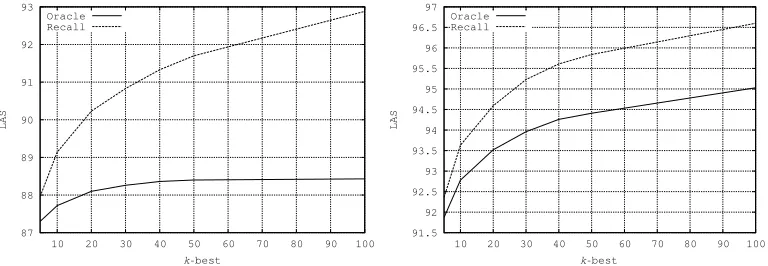
In order to compare the search spaces respectively defined by ak-best parse list and the correspondingD_kset, we define two measures on thek-best parse list. The first one (Oracle LAS) corresponds to the LAS of the best tree in thek-best list. The second one (Recall LAS) is the part of labeled dependencies of the reference parse that appear in

D_k. Oracle LAS constitutes an upper bound for reranking and Recall LAS is an upper bound for combination. The values of these two measures are represented in Figure 3

Figure 3

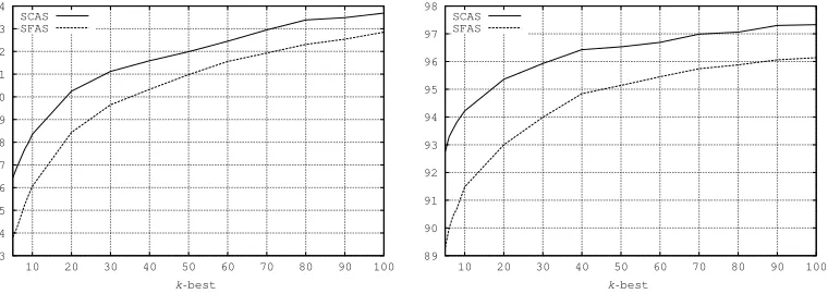
Figure 4

Recall SFAC and SCAS of thek-best trees for first-order (left) and second-order (right) parsing, computed on FTB TEST.

for first-order parsing (left) and second-order parsing (right) measured on the test set of the French Treebank.

As one can see in Figure 3, the Recall LAS curve is, of course, always above the Oracle LAS curve. In the case of first-order parsing, the Oracle curve quickly reaches a plateau. This is because first-orderk-best parses are generally very close to one another, because of the very local nature of the model. The parses in the k-best list tend to be combinations of dependencies that appeared in previous parses. The number of new dependencies created tend to decrease quickly withk. Fork=100, the difference between the Oracle and the Recall scores is almost equal to 5 points. This difference clearly demonstrates the advantage of usingD_kinstead of thek-best list.

The results for second-order parsing are less spectacular. The Oracle curve does not reach an asymptote, as it was the case for first-order parsing. New dependencies are continually being created askincreases. The reason why we have considered first-order models in this section is that generating a first-first-orderk-best solution can be done very efficiently; second-order k-best generation is more time-consuming. Performing candidate generation with a first-order parser is therefore a potentially interesting method. We will see in the two following sections that first-orderk-best generation gave good results on French but did not perform well on English, where second-orderk-best generation had to be used.

Although Figure 3 gives an estimation of the LAS upper bounds of reranking and combination, it does not tell us what can be expected in terms of SFAS and SCAS. Figure 4 answers this question by showing the evolution of Recall SFAS and Recall SCAS on the same data set. As one can see, for k=100, with first-order k-best generation, almost 94% of the ISCs and 93% of the ISFs that appear in the reference can be recovered. The results for second-orderk-best are, respectively, equal to 97% and 96%.

7. Experiments on French

Table 1

Decomposition of the French Treebank into training, development, and test sets.

number of sentences number of tokens

FTB TRAIN 9,881 278,083

FTB DEV 1,239 36,508

FTB TEST 1,235 36,340

the extracted data. The results of patching and parsing are given in Section 7.3 and an analysis of the errors is presented in Section 7.4. Section 7.5 analyzes the runtime performances.

7.1 Parsing

The parser was trained on the French Treebank (Abeill´e, Cl´ement, and Toussenel 2003), transformed into dependency trees by Candito et al. (2009). The size of the treebank and its decomposition into train, development, and test sets are represented in Table 1.

The parser gave state-of-the-art results for French: the LAS and UAS are, respec-tively, 88.88% and 90.71%. The SCAS reaches 87.81% and the SFAS is 80.84%, which means that in 80.84% of the cases, a verb selects its correct subcategorization frame. These results are for sentences with gold part-of-speech-tags and lemmas.

An analysis of the errors shows that the first cause of errors is prepositional attach-ments, which account for 23.67% of the errors. A more detailed description of the errors is given in Table 2. Every line of the table corresponds to one attachment type. The first column describes the nature of the attachment. The second indicates the frequency of this type of dependency in the corpus. The third column displays the accuracy for this type of dependency (the number of dependencies of this type correctly predicted by the parser divided by the total number of dependencies of this type). The fourth column shows the contribution of the errors made on this type of dependency to the global error rate. We have used this error analysis to define the following four SC patterns, which we call SBJ, OBJ, VdeN, and VaN:

SBJ ([:V:::]([SUJ:N:::])) OBJ ([:V:::]([OBJ:N:::]))

VdeN ([:V:::]([DE-OBJ:P:de::]([OBJ:N:::]))) VaN ([:V:::]([A-OBJ:P:a::]([OBJ:N:::])))

The last column of Table 2 indicates the SC pattern that corresponds to a given type of error. One can see that all SC patterns are not described at the same level of detail—some of them specify the label of the dependency, if considered important (to distinguish subject and object, for example), and others specify the lexical nature of the dependent (for prepositions, for example).

7.2 Extracting SFs and SCs

Table 2

The seven most common error types made by the baseline parser. For each type of error, we displayed its frequency, the parser accuracy, the impact on global errors, and the SC pattern that corresponds to the error type.

dependency freq. acc. contrib. SC pattern

N—mod→N 1.50 72.23 2.91

V—∗ →`a 0.88 69.11 2.53 VaN V—suj→N 3.43 93.03 2.53 SBJ N—coord→CC 0.77 69.78 2.05

N—∗ →de 3.70 92.07 2.05

V—∗ →de 0.66 74.68 1.62 VdeN V—obj→N 2.74 90.43 1.60 OBJ

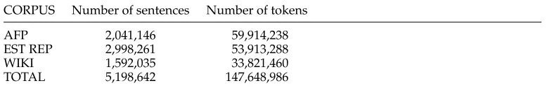
The third (WIKI) is a collection of articles from the French Wikipedia. The size of the different corpora are detailed in Table 3.

The raw corpora were first tokenized, POS-tagged, and lemmatized with the MACAON tool suite (Nasr et al. 2011), then parsed in order to get the most likely parse for every sentence. The SFs and SCs were then extracted from the parses and their scores computed. In the two following sections, we give some statistics on the SFs and SCs produced.

7.2.1 Extracted SF.As described in Section 3.3, an SF frame is a special kind of LSC. Its root is a predicate and its leaves are the arguments of the predicate. Some linguistic constraints are defined over SF. The first one is the category of the root, which must be either a finite tense verb (V), an infinitive form (VINF), a past participle (VPP), or a present participle (VPR). The second is the set of syntactic functions that introduce arguments of the predicate; they can either be a subject (SUJ), a direct object (OBJ), or an indirect object introduced by preposition`a(A-OBJ) orde(DE-OBJ).

SFs are defined at a level that is slightly more abstract than the surface syntactic realization. Two abstractions are in action. The first one is the factoring of several parts of speech. We have factored pronouns, common nouns, and proper nouns into a single category N. We have not gathered verbs of different modes into one category because the mode of the verb influences its syntactic behavior and hence its SF. The second abstraction is the absence of linear order between the arguments.

The number of verbal lemmas, number of SFs, and average number of SFs per verb are shown in Table 4, columnA0. As can be observed, the number of verbal lemmas and

Table 3

Some statistics computed on the corpora used to collect Subcategorization Frames and Selectional Constraints.

CORPUS Number of sentences Number of tokens

AFP 2,041,146 59,914,238

EST REP 2,998,261 53,913,288

WIKI 1,592,035 33,821,460

Table 4

Number of verbal lemmas, SFs, and average number of SFs per verb for three levels of thresholding (0, 5, and 10).

A0 A5 A10

number of verbal lemmas 23,915 4,871 3,923 number of different SFs 12,122 2,064 1,355 average number of SFs per verb 14.26 16.16 13.45

SFs are unrealistic. This is because the data from which SFs were extracted are noisy: they consist of automatically produced syntactic trees that contain errors. There are two main sources of errors in the parsed data: the pre-processing chain (tokenization, part-of-speech tagging, and lemmatization), which can consider as a verb a word that is not; and, of course, parsing errors, which tend to create incorrect SFs. In order to fight against noise, we have used a simple thresholding: We only collect SFs that occur more than a thresholdi. The results of the thresholding appear in columnsA5andA10, where the subscript is the value of the threshold. It is a very crude technique that allows us to eliminate many errors but also rare phenomena. As expected, both the number of verbs and SFs decrease sharply when increasing the value of the threshold. The average number of SFs per verb is 14.26 without threshold and reaches 16.16 for a threshold of 5. This phenomenon is mainly due to part of speech tagging errors on the raw corpus: A large part of hapax are words mistakenly tagged as verbs. They disappear with thresholding, and their disappearance tends to increase ambiguity.

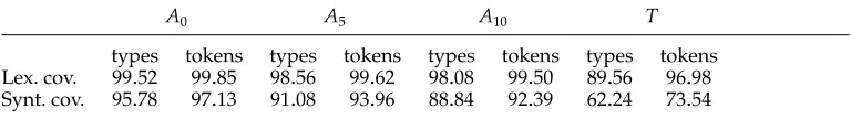
We report in Table 5 the coverage of the extracted SFs on FTB DEV. The last column represents the coverage of the SF extracted from FTB TRAIN. These figures constitute an interesting reference point when evaluating the coverage of the SFs extracted from raw data. We have distinguished lexical coverage (ratio of verbal lemmas of FTB DEV present in the resource) and syntactic coverage (ratio of SFs of FTB DEV present in the resource). Both measures were computed on types and tokens. Table 5 shows that lexical coverage is very high, even onA10. It is interesting to note that syntactic coverage of the automatically built resource is much higher than syntactic coverage of the same resource extracted from FTB TRAIN. This clearly shows that many SFs of FTB DEV were not seen in FTB TRAIN. This observation supports our hypothesis that treebanks are not large enough to accurately model the possible SFs of a verb. Comparing coverage ofTand Ax is somehow unfair because, as we already mentioned, the automatic resources are noisy, and have a tendency to overgenerate whereasTcontains only correct SFs (up to the corpus annotation errors). Accuracy results of Section 7.3 will give a more balanced

Table 5

Lexical and syntactic coverage on FTB DEV of the extracted SFs. Coverage is computed for three thresholding levels of the automatically generated resource (A0,A5, andA10) and FTB TRAIN (T).

A0 A5 A10 T

Table 6

Number of occurrences of the four SC patterns (OBJ, SBJ, VdeN, and VaN) in raw corpora with three levels of thresholding (0, 5, and 10).

SC pat. A0 A5 A10

OBJ 422,756 58,495 26,847 SBJ 433,196 55,768 25,291 VdeN 116,519 11,676 4,779 VaN 185,127 23,674 10,729 TOTAL 1,157,598 149,613 67,646

view by computing how many errors are actually corrected using the noisy extracted resource.

7.2.2 Extracted SCs. The number of different SCs extracted for each of the four SC configurations are shown in Table 6 for the three thresholds 0, 5, and 10.

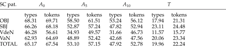
The coverage of SCs on FTB DEV is shown in Table 7. It is interesting to note that SC coverage is much lower than SF coverage. This is due to the different nature of the two phenomena: SC is a bilexical phenomena whereas SF is a monolexical one. Ideally, a larger corpus should be used to extract SCs. One can also note that the coverage of SCs extracted from FTB DEV is very low.

7.3 Results

The results obtained by our method are shown in Table 8, using the four measures defined in Section 6.1. The accuracy scores of the baseline parser are presented in line 1. Line 2 shows the results obtained when setting parametersµ₁andµ₂to 1. This setting corresponds to the situation where SF and SC scores are not used. Patching, in this case, only combines ILSCs that have a good confidence measure. This experiment is important in order to ensure that sSF andsSC do carry useful information. As one can see, settingµ₁andµ₂to 1 slightly increases the accuracy of the parser, which means that the accuracy of the parser can be increased just by imposing the final parse sub-parses that have a good confidence measure.

The optimal values ofµ₁ andµ₂ were computed on FTB DEV; they are both 0.65. These values are used for the experiments corresponding to lines 3, 4, and 5. Lines 3

Table 7

Coverage for the four SC configurations (OBJ, SBJ, VdeN, VaN). Coverage is computed for three thresholding levels of the automatically generated resource (A0,A5, andA10) and FTB TRAIN (T).

SC pat. A0 A5 A10 T

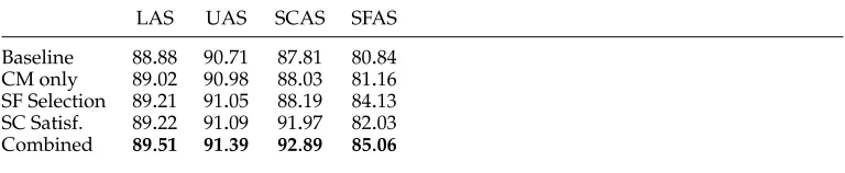
Table 8

Four measures of accuracy on FTB TEST for four settings: Baseline second-order parser, patching with confidence measure, patching with SF only, patching with SCs only, and patching with SFs and SCs.

LAS UAS SCAS SFAS

Baseline 88.88 90.71 87.81 80.84 CM only 89.02 90.98 88.03 81.16 SF Selection 89.21 91.05 88.19 84.13 SC Satisf. 89.22 91.09 91.97 82.03 Combined 89.51 91.39 92.89 85.06

and 4 indicate the accuracy for SF selection and SC satisfaction alone, as described in Sections 3.3 and 3.4. Line 5 provides the result when they are combined, as described in Section 3.5.

The table shows that, when setting µ₁ and µ₂ to their optimal values, the three methods increase both LAS and UAS with respect to the baseline. The best results are obtained by the combined method. SCAS and SFAS allow us to gain a better under-standing of what is happening. As could be expected, SF selection has a stronger impact on SFAS whereas SC satisfaction has a stronger impact on SCAS. But both methods also have a positive influence on the other measure. This is because SFs and SCs are not independent phenomena and correcting one can also lead to correcting the other. The combined method yields the best results on our four measures.

7.4 Error Analysis

There are three main causes for SC and SF errors: insufficient coverage ofL, narrowness of the patching search spaceI, or inadequacy of the ILP objective function. Given a sentenceS, let us note R its correct parse andH the parse produced by our system. Let us note ˆI_R and ˆI_H, respectively, the set of ILSCs ofRandH. We define an error as an ILSCx∈Iˆ_R, such thatx∈/Iˆ_H, and we notey the LSC corresponding to x (xis an instantiation ofy). The three error causes are described as follows:

NotInDB y∈/L. This is the situation where an ILSC cannot be extracted from the k -best list because its corresponding LSC does not appear inL. A possible cause for such errors comes from the corpora we have used to extract LSCs. We have shown in Section 7.2 that the coverage of our resources is not perfect and some ILSCs that appear in the reference parseRmight not appear in the resource. A solution to such a problem would be to use larger corpora in order to increase coverage. Another cause of this error is the processing chain that was used to process the raw corpora. As already mentioned, any of the modules that compose this chain can make errors and introduce noise inL.

Table 9

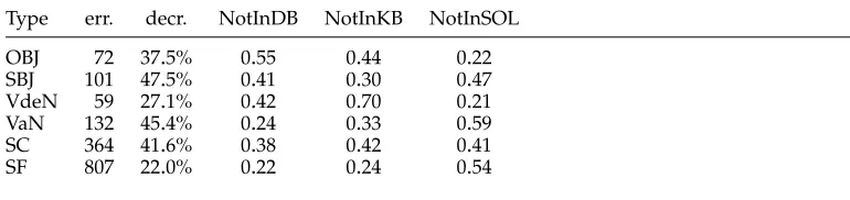
Raw number of errors, error decrease, and error distribution for each SC pattern, average of SC patterns, and SFs.

Type err. decr. NotInDB NotInKB NotInSOL

OBJ 72 37.5% 0.55 0.44 0.22 SBJ 101 47.5% 0.41 0.30 0.47 VdeN 59 27.1% 0.42 0.70 0.21 VaN 132 45.4% 0.24 0.33 0.59 SC 364 41.6% 0.38 0.42 0.41 SF 807 22.0% 0.22 0.24 0.54

the search space yields larger IL programs and therefore the resolution time of the ILP.

NotInSOL x∈I∪I0 but x∈/Iˆ_R. This is the situation where x is in the input of the ILP program but is not part of the solution. There are two possible causes for this situation. The first one comes from the scoressSFandsSCcomputed on the corpora. A correct ILSC might have been assigned a lower score than an incorrect one. This situation, in turn, can be due to different attachment preferences in the test and the raw corpora used to produceL. The second cause is the confidence measure used to introduce a syntactic dimension to the ILP objective function, as described in Section 4. In some cases, an ILSC might have a good lexical score but a bad syntactic score, in which case it is ruled out.

Table 9 details the distribution of the errors over these three categories. Column 1 describes the nature of the attachment. The four first rows correspond to specific SC patterns, row 5 is the average of all SCs, and row 6 concerns SF selection. Column 2 indicates the number of errors made by the baseline parser. Column 3 indicates the decrease of the number of errors and columns 4, 5, and 6 give the distribution of the errors over the three error types defined earlier.

As one can see from Table 9, our method decreases by 41.6% the number of SC errors and by 22% the number of SF errors. The difference between these two figures comes from the fact that SFs are more complex phenomena that SC patterns. SFs can be composed of a large number of dependencies and an error in one of them leads to an error in the SF selection.

The SC errors are almost equally distributed along the three error types: In 38% of the cases, the correct SC is notL; in 42% of the cases, the correct SC does not appear in the 100 best parses; and in 41% of the cases, the ILP fails to find the correct SC, although it is in the search space. There are three possible causes for the latter type of error: Recall that the objective function of the ILP is based on the scores of ILSCs, which are them-selves a combination of a lexical and a syntactic score:s(∆)=(1−µ)sL(∆)+µsS(∆). The cause of the error could be the lexical score (sL), the syntactic score (sS), or the weight (µ).

Figure 5

Decomposition of runtime on FTB TEST.

7.5 Runtime Analysis

Figure 5 displays the runtime of our system with respect to the length of the sentences parsed. Runtime has been decomposed in three parts: first-order 100-best generation, ILP solving, and constrained second-order parsing. The runtime of the instantiation process is not reported because it is negligible compared with the runtime of the other processes.

Figure 5 shows that ILP resolution is the most time-consuming part of the whole process. Although in practice the performances of the whole system are reasonable (approximately 330 words per second on average), we show that the patching problem is NP-complete and we have no guarantee that the problem will be solved in polynomial time.

8. Experiments on English

A second series of experiments was performed on English. Although the setting used is almost the same as for French, there are some notable differences between the two series of experiments with respect to the data used:

r

r

r

8.1 Parsing

Table 10

Decomposition of the Penn Treebank into training, development, and test sets.

Number of sentences Number of tokens

PTB TRAIN (Sec. 02–21) 39,279 958,167

PTB DEV (Sec. 22) 1,334 33,368

PTB TEST (Sec. 23) 2,398 57,676

into training, development, and test sets, with sizes as reported in Table 10. The main difference with respect to French comes from the training set, which is 2.44 times larger. As could be expected, the parser trained and evaluated on the Penn Treebank yields better results than the same parser trained on the French Treebank. The LAS is 91.76 and UAS is 93.75, a relative increase of 3.24% and 3.35% with respect to French.

The English SF and SC definitions differ from the French ones in the choice of the preposition used. The nine most frequent prepositions occuring in the Penn Treebank were taken into account ({of, in, to, for, with, on, at, from, by}) to define both SCs and SFs. A set of 20 SC patterns are defined:{OBJ, SBJ, VofN, VinN, VtoN, VforN, VwithN, VonN, VatN, VfromN, VbyN, NofN, NinN, NtoN, NforN, NwithN, NonN, NatN, NfromN, NbyN}. SFs are defined as the dependents of a verb that are introduced by one of the nine prepositions, plus the subject and the object.

The SCAS and SFAS are, respectively, 91.99 and 88.24: an increase of 4.76% and 9.15% compared to French. These results show that the English parser makes fewer errors on prepositional attachments. This situation may be due to the fact that prepo-sitional attachments are more ambiguous in French (4.56 prepositions on average per sentence in the FTB compared with 3.15 for the PTB).

Table 11 details the error rate for each of the 20 SC patterns defined, sorted with respect to their contribution to the total error rate. The total contribution of these errors reaches 18.87%, which is an approximation of the upper limit of the improvement that we can expect from our method. The mean accuracy for these patterns is almost equal to 92%. Two situations should be distinguished, however: the subject and direct object dependencies, on the one hand, and the prepositional attachments, on the other. The

Table 11

Contribution of the 20 SC patterns to the errors made by the parser. For each pattern, we displayed its frequency, the parser accuracy, and the impact on global errors.

SC pat. freq. acc. contrib. SC pat. freq. acc. contrib.