Multiphase Particle Simulation of Gas Bubble Passing
Through Liquid
/
Liquid Interfaces
Shungo Natsui
+, Hifumi Takai, Takehiko Kumagai, Tatsuya Kikuchi and Ryosuke O. Suzuki
Division of Materials Science and Engineering, Faculty of Engineering, Hokkaido University, Sapporo 060-8628, JapanA newly developed computationalfluid dynamics (CFD) model based on a multi-phase particle method is presented for predicting the entrainment behavior of liquid metal into slag due to rising single bubble. By comparing results calculated using this model against experimental data, it was found that the transient behavior of bubbles and the two immiscible liquids can be accurately estimated by this method. The rupturing of the thin waterfilm surrounding the bubble was less reliably predicted, but this 3-dimensional unsteady numerical model still nevertheless provides valuable new information for directly predicting the change in the liquid/liquid interface over time. Such prediction of continuous change in an interface has not been possible by more conventional methods, and thus further improvement in the accuracy of this simulated model may well be the only way to non-empirically predict the metal-slag interface area in actual processes.
[doi:10.2320/matertrans.M2014245]
(Received July 2, 2014; Accepted August 11, 2014; Published September 20, 2014)
Keywords: molten metal, slag, gas bubble, liquid/liquid interface, computationalfluid dynamics, particle method simulation
1. Introduction
In many pyrometallurgical processes, the molten metal-slag interface plays an important role in increasing the rate of chemical reaction and the efficiency of refining. Given the immiscibility of these two liquids and the high temperatures typically involved, stirring is normally achieved by a flow of gas. The behavior of these gas bubbles when they are coated with a metal layer and passed through the molten slag is therefore intimately associated with the overall reaction rate. For example, the O2 gas injected into a steelmaking
converter determines the decarburization, dephosphorization, and desiliconization reactions.1,2) Similarly, in a copper
smelting converter, droplets of molten metal sulfide matte are generated by SO2 gas, and are subsequently suspended
at the slag/atmosphere surface; a phenomena referred to as mechanical copper loss.3,4)
Given the very real practical significance of the passing behavior of a gas bubble rising through a liquid/liquid interface, there has been considerable research attention given to more fully understanding this phenomenon. Amongst the earliest examples of such research includes the investigation of metal entrainment mechanisms by Davenport et al. using mercury/water-glycerin (20°C), lead/molten salt (520°C) and copper/slag (1200°C) sys-tems.5,6)This identified that the metal is entrained in the slag
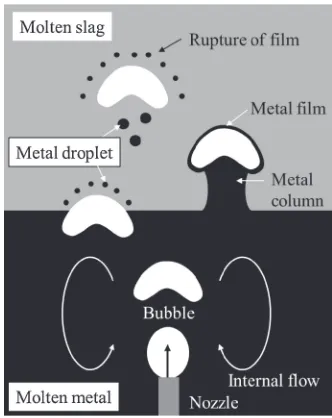
mainly through rupture of the metal coating on the gas bubble. More recent investigations using low temperature media have shown that a metal column generated below the bubble can sometimes penetrate fully into the upper slag layer before it finally collapses.7,8) This behavior of the bubble and liquid/liquid interface is shown in schematically Fig. 1; however, Song et al.9) have proposed an additional rupture phenomenon, wherein an elongated metal column is formed by two or three bubbles passing through the interface of an Al-Cu alloy/molten salt system (700°C). Here, a metal dome isfirst formed at the interface by the rising gas bubble, with successive bubbles reaching this interface before the
initial bubble is detached causing the metal column to extend further into the slag phase. Observations of the same material in an actual high temperature process have also been attempted, with Terashimaet al.10) analyzing matte droplets
on the slag surface using a floating particle model and penetration X-rayfluoroscopy (1200°C). Similarly, the iron/ slag (14501500°C) interface has been directly observed under specific conditions,11,12) though quantitative and
detailed descriptions of its behavior at high temperature are rare.
Understanding the dynamic behavior of a liquid/liquid/ gas interface is complicated by its dependence on a combination of several physical properties: density, viscosity, interfacial energy, velocity, shape, etc. Consequently, although many quantitative analyses have been attempted, it is still extremely-difficult to accurately predict the liquid/ liquid interface behavior through experimental data alone. Unfortunately, 3-dimensional dynamic analysis of the inside Fig. 1 Schematic diagrams of bubbles passing through molten metal and
slag.
[image:1.595.343.509.312.521.2]of a molten metal and slag has also proven difficult to apply due to an extremely limited observation domain; i.e., the behavior of a 3-dimensional bubble cannot be determined from 2-dimensional observations. Reiteret al.were success-ful in using the iron entrainment phenomena observed in a cold scale model to quantitatively relate mass transfer to physical entrainment;13,14) however, the liquid/liquid inter-facial area in this instance was estimated by local rotational symmetry approximation, and the accuracy was not described in detail.
With recent progress in computational science and technology, there is a possibility that high-accuracy numer-ical simulation could provide a solution to understanding the transient behavior of liquid/liquid interfaces. The volume of fluid (VOF) method15)is already well known, and relies on a
Eulerian approach to determine the relative amount of each fluid through computationalfluid dynamics (CFD). However, in the case of a liquid dispersion and advection of bubbles, the VOF method requires a special numerical diffusion technique in order to prevent an accumulation of errors caused by the coarse grain size of the interface. This can be overcome by using a fully-Lagrangian mesh-free particle method, which discretizes thefluid as moving particles. This results in a simpler algorithm, as each particle keeps the interface sharp. The gravity separation of a bubbly water/oil flow has also been studied by Grenier et al. using a novel multi-fluid smoothed particle hydrodynamics (SPH) ap-proach.16)Of all the simulation methods available, however,
it is the moving particle semi-implicit (MPS) method17)that is
perhaps the most promising. This was originally developed for use with incompressiblefluids, but was later expanded for use with solid and fluid mechanics. Indeed, in the author’s last article, this was used to improve the stability of a gas/ liquid interface and was shown to provide good computa-tional accuracy when compared with analytical/experimental results.18)Expanding on this work, this paper aims to develop a physical model for the penetrating of a single bubble penetrating into a metal/slag interface based on a multi-phase particle method, and to verify its accuracy by comparing against experimental results obtained by a laboratory-scale cold model.
2. Method
2.1 Numerical modeling of thefluid
Using the particle method, fluid flow is tracked by discretized particles in a Lagrangian system, wherein all fluids (liquid and gas) are assumed to be incompressible due to a sufficiently small Mach number. The fluids are then spatially discretized by particles with a density ofµ; however, the varying density of a gas/liquid flow requires that µ
be defined as a density function for each particle by the equation:
µi¼ hµii ð1Þ
where © ª represents the interparticle interaction, i.e., that particle i is influenced by its surroundings and the density of the fluid varies with spatial distribution. The large density difference at a twophase interface also dramatically affects the momentum exchange, and thus an interface density
function is introduced in the boundary particles to smooth the pressure gradient between the two phases:
hµii¼X
j6¼i
mjwij
Z
V
wijdV ð2Þ
where mjis the mass of particle j,w is the weight function
and Vis the volume of thefluid. The basic premise of the MPS method is to express motion in an incompressiblefluid by keeping the ambient density of each particle constant. The sum of the weight functions of neighboring particles is then defined as the particle number density,n:17)
hnii¼
X
j6¼i
wij;wij¼
re
rij 1 ðrijreÞ
0 ðrij> reÞ
8 <
: ð3Þ
whererijis the distance between particles i and j (=«rj¹ri«),
and reis the radius of influence of the weight function. In
this study, an re=2.1dp is assumed.19) To maintain the
incompressibility of thefluid, a standard particle density,n0,
is given by the initial arrangement of uniformfluid particles:
n0 ¼X
j6¼i
wij0 ð4Þ
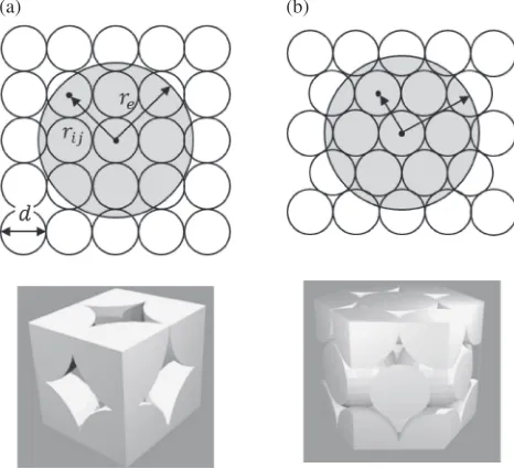
Since all particles try to maintain a constant density and remain as close as possible to n0, this directly affects the numerical stabilization of the pressure distribution. Figure 2 shows the initial arrangements of particles, in which a simple cubic (SC) arrangement is used and the filling fraction is relatively low (fµ0.52). With gas/liquidflow, the particles move easily under the pressure gradient induced; i.e., the ratio of density between gas and liquid is approximately
1 : 1000. In a previous report, a checkerboard (CB) arrange-ment was introduced that has a highfilling fraction, thereby partially reducing the pressurefluctuation. As the same time, a hexagonal close-packed (HCP) arrangement was employed to facilitate a more stable calculation, as shown in Fig. 2. In this, a denser noncompressed state is assumed, and thus the numerical stability of the gasliquid interface can be improved.
Theflow of eachfluid phase is governed by the continuity equation and the NavierStokes equation for incompressible fluids:
Dµ
Dt þµr u¼0 ð5Þ
Du
Dt ¼
1
µrpþ¯r2uþgþ 1
µFs ð6Þ
whereuis the velocity,tis the time,pis the pressure,¯is the kinetic viscosity, g is the force of gravity, and Fs is the
surface tension expressed in terms of force per unit volume of fluid. Equation (6) is discretized by the MPS method, by which the pressure gradient is calculated by an implicit method, whereas all other terms are calculated by an explicit method:
Du
Dt ¼
1
µrp
tþt
þ ½¯r2utþ ½gtþ 1
µFs
t
ð7Þ
u¼utþt ¯r2uþgþ1
µFs
t
ð8Þ
Whereu is the velocity in the prediction step. The pressure term remains an unknown value, and is therefore solved using the particle number density in the prediction stephnii, which in turn is explicitly solved using the particle velocity and initial particle density. Both the gas phase and liquid phase are discretized by particles in this model, often leading to an increase in numerical destabilization due to the very different density of the gas/liquid interface. This is caused by keeping strict compressibility at the interface, and thus a limited compressibility is assumed to stabilize the pressure at the interface. Moreover, since a smooth density function©µªi
is specified at the gas/liquid interface, it should not be given as a constant. A spatial differentiation of©µªiis therefore also
considered in this model, with the following equation of Poisson employed:
r hµ1i
irp tþt i
¼r u
t
£ t2
hni
i
n0
1
ð9Þ
This formulization is similar to the stable algorithm used for calculating compressible flow by an Eulerian approach. A convergent calculation is applied instead of an explicit calculation to ensure interfacial stability can be obtained. Considering the numerical stability and volume conserva-tion,18)a value of£=0.01 was employed, with the velocity
of each particle then obtained using ptiþt:
utþt¼uþ t
µ rpi
tþt
ð10Þ
The particle-particle interaction forcesFsare then added to
the momentum conservation equation to generate the surface tension. A continuum surface force (CSF) model was localized to the fluid interface by applying it to fluid elements in the transition region of the interface.20) The
surface tension is then converted to a force per unit volume by:
Fs,i¼¤ifs,i;¤i¼ 1 ðNi<¢N 0Þ
0 ðNi¢N0Þ
ð11Þ
Where ¤ is a delta function for the judgment of surface particles, in which the neighboring same-phase particle number Ni is used. Here, ¢ and N0 are the coefficient for
surface judgment and the standard neighboring particle number in an incompressible state and respectively. In the present research a value of¢=0.85 was assumed,19)and the force per unit area (fs) was given by the interparticle potential
force model. According to previous research, the exact form of this force is not important provided it is anti-symmetric and short-range repulsive, or long-range attractive.21)In this
study,fswas constructed following the previous study,22)who
employed this same type of interaction force to dissipative particle dynamics (DPD) models:
hfsii¼ 2·dp2
X
j6¼i
ºðrijÞ
!1
ðrijdÞðrijreÞ ð12Þ
where · is the surface tension coefficient, and º is the interparticle potential. Natsui et al.22)verified that this form can estimate the absolute value of surface tension; and in the case of multi-phaseflow, different phases are formed in pairs with interface particles, as shown in Fig. 3. Meanwhile, at the surface, the two interface particles should maintain a smooth pairwise relation. Here, the two different liquid phases are defined as A and B. If we therefore consider a liquid A particle in contact with gaseous particles, it can be assumed that the surface tension·ichanges smoothly in relation to the
particle number ratio between liquid A and B. This can be given as:
·i¼ h·ii ð13Þ
then,
h·ii¼Nij·AþNik·B
NijþNik ð14Þ
WhereNijis the number of particlesjð3AÞaround particle i
that are in contact with gaseous particles,Nikis the number of
particles kð3BÞ around particle i that are in contact with gaseous particles, ·A is the surface tension coefficient of
liquid A, and·Bis the surface tension coefficient of liquid B.
Thanks to this simple assumption, which accurately predicts Fig. 3 Schematic diagram of the forcefield in a gas/liquid/liquid triple
phase interface.
(a) (b)
[image:3.595.311.545.65.229.2] [image:3.595.52.285.73.285.2]a water/oil system, the surface tension at the A-gas and B-gas interfaces changes smoothly. This “mutual interface”model was employed for gas/liquid/liquid simulation, in which the liquid/liquid interface tension coefficient·AB remains as an
unknown value. It is subsequently derived by applying
“Antonoff’s rule”:23)
·AB¼ j·A·Bj ð15Þ
2.2 Calculation conditions
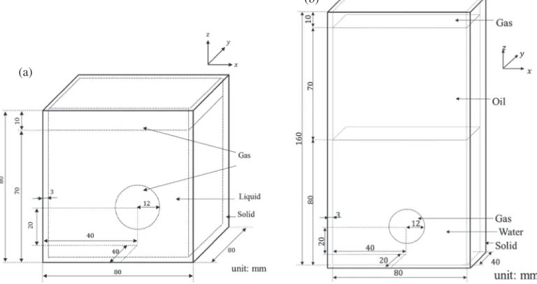
Calculation tests were carried out for each of the multi-phase fluid systems, with the calculation domain shown in Fig. 4. This method was first applied to an actual gas liquid system, as shown in Fig. 4(a), which was aimed at examining the rise, modification, and bursting of a single bubble at the liquid surface. Next, we attempted to apply this model to a gas/liquid/liquid multi interface system, as shown in Fig. 4(b). The calculation conditions are shown in Table 1, with the particle diameter remaining constant. Dissolution of the gas to liquid was completely ignored. The programs used in this research were all custom written by the authors in Fortran90/95, and then compiled using Intelμ Fortran Composer Version 14.1. To reduce the calculation time, parallel processing of the program code was implemented using OpenMP. The CPU used in this work was an IntelμCore i7-4820K (3.7 GHz, 4 cores).
2.3 Experimental
The simulation results were verified by comparison with an isometric experiment, with a schematic illustration of the apparatus used for this given in Fig. 5. In this, an acrylic tank wasfirstfilled with liquid, and then a constant volume of air was injected through a plastic tube by a syringe pump. The air was trapped in a hemispheretype dumping cup (0.030 m in diameter, plastic), to which was attached a nichrome rod that was rotated by 180° to modify the shape of the bubble and allow it to rise. Changes in the interface were recorded at a rate of 1500 frames per second and a resolution of 1024©1024 pixels using a highspeed video camera (Fastcam SA3 model, Photoron Co., Ltd.). For each image capture, the location of the the tip of the bubble was analyzed using image processing software (PFV viewer ver. 338).
3. Results and Discussion
3.1 Gas/liquid system
The change in the maximum height of the liquid (distilled water) and diameter of the gas bubble over time are shown in Fig. 6. From this we see that the bubble rises due to the buoyancy generated by the density difference between the gas and the liquid; while at the same time, it also becomes elongated horizontally. This behavior agrees well with the results of a previous report,18) which is attributed to the
initial HCP particle arrangement and mutual interface model
(a)
(b)
[image:4.595.106.490.77.280.2]Fig. 4 Schematic diagrams of the computational domain and initial configuration.
Table 1 Calculation and experimental conditions.
Fluid water oil (10cs) oil (100cs) air
Density,µ kg/m3 997 935 965 1.18
Kinetic viscosity¯ m2/s 8.93©10¹7 1.00©10¹5 1.00©10¹4 1.54©10¹5
Surface tension· N/m 7.20©10¹5 2.01©10¹5 2.09©10¹5 ®
Bubble volume,V m3 7.31©10¹6
Time step,dt s 1.0©10¹5
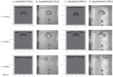
[image:4.595.46.554.324.430.2]stabilizing the bubble behavior. The influence of the liquid’s viscosity on bubble behavior is shown in Fig. 7 by a series of images obtained through simulation and experimentation in 10cs and 100cs silicone oils. It should be noted that even though the experimental data shows a twodimensional representation of a transparent object, it nevertheless can be clearly seen that a domeshaped bubble rises in the liquid at t=0.10 s, changes att=0.15 s, and then reaches the liquid
surface at t=0.20 s. More importantly, it shows that the viscosity of the liquid directly affects the bubble shape, with a higher high viscosity resulting in a more vertically elongated shape. Figure 8 shows a quantitative comparison of the change in bubble height and shape over, in which it is revealed that although the upward velocity of the bubble remains much the same, its movement is delayed in the 100cs at t=0.15 (Fig. 8(a)). The difference between these two Fig. 6 Comparison of experimental and calculated results for the change over time in the maximum water heightHw, and the widthDxand height
Dzof the air bubble.
Fig. 7 Snapshots of a gas bubble rising through silicon oil. In the simulation results, black particles represent the gas phase, dark grey particles the liquid phase, and light grey particles the solid phase.
[image:5.595.67.271.69.306.2] [image:5.595.311.536.70.310.2] [image:5.595.100.491.364.633.2]liquids is more pronounced when considering the aspect ratio of the bubble (Fig. 8(b)). For instance, the 10cs oil causes Dx/Dzto increase smoothly; whereas this remains constant in
the 100cs oil untilt=0.15 s, after which it increases rapidly. The calculated results show good agreement with these experimental results, and in doing so confirm the effective-ness of this model in predicting bubble movement by viscous flow.
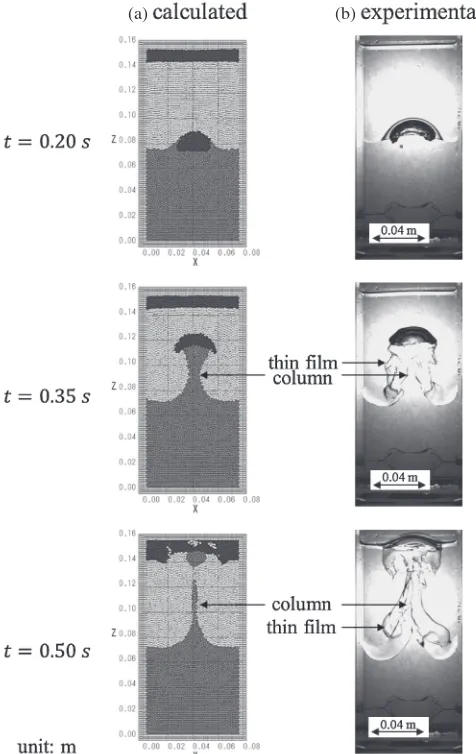
[image:6.595.117.479.70.263.2]3.2 Gas/liquid/liquid system
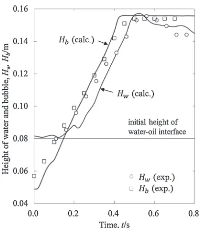
Figure 9 shows snapshots of a bubble rising through a water/oil interface obtained by simulation and experimenta-tion. At t=0.20 s, we see that the rising bubble starts to modify the water/oil interface by pulling the water phase upwards through the oil/water interface. The height of the water column generated steadily increases until a neck is formed at around z=0.09 m, with this tendency described quantitatively in Fig. 10. The bubble height shows good agreement with the experimental data, suggesting that change in the shape of the interface by convection can be correctly estimated. On the other hand, the height of the water column obtained by calculation shows a later increase than was observed in the experiment, and the simulated liquid surface was slightly thinner at t=0.20 s in Fig. 9. This can be explained by the finite interface thickness used in this simulation, which results in rapid rupture of a “thin water film”. The error resulting from this thinfilm is most evident after the air bubbles enter the interface, with the experimental data showing a thin waterfilm present on the front and back side at t=0.35 and 0.50 s. The formation of this thin film on the liquid surface is therefore either disregarded by the calculation conditions used, or the liquid/liquid interface tension is insufficient to accurately predict.24) However, by
using this method, convection phenomena of three phase were successfully calculated without numerical diffusion. Further large scale simulation can simultaneously predict the thin waterfilm and convection.
Three-dimensional gasliquid interfaces are shown in Fig. 11, in which the changes evident with even a simple single bubble make it clear that the 2-dimensional
informa-tion obtained from the cold model experiment is insufficient to fully predict the behavior of an actual gas/liquid/liquid interface. In order to help show the change of 3-dimensional
(a) (b)
Fig. 8 Experimental and calculated results for the change over time in the height and diameter of a bubble in different oils.
(a) (b)
[image:6.595.305.543.309.686.2]interface, only the water phase was displayed. The main novelty of this research is therefore its direct prediction of the liquid/liquid surface areaAfrom its initial conditionA0and
the surface delta function:
A A0
t
¼ X
i
¤i
" #t X
i
¤i0 ð16Þ
[image:7.595.67.270.66.298.2]Figure 12 shows the fluctuating increase in the areas of a simulated liquid/liquid surface over time, up until the point at which the thin water film separating the two ruptures (Fig. 12a). Note that although A is decreases temporarily after this rupture of the thinfilm, it is significantly increased with subsequent growth of the water column. From this, it is concluded that even a single bubble can stir a liquid/liquid interface. Moreover, the maximum value of A is achieved when the bubble reaches the surface of the oil att=0.45 s, as this is when the growth of the water column finally stops (Fig. 12b). Subsequent coalescence of the water droplet in the oil causes Ato decrease, with the slow sedimentation of the droplets eventually causing the area to remain steady at a value ofA/A0³1.20. Thus, a bubble continues to affect the interface area, even after passing through it.
[image:7.595.105.493.360.770.2]Fig. 10 Change in the maximum height of the water and bubble over time.
4. Conclusion
A new particle-method computational fluid dynamics model was developed for molten metal-slag-gas multi-phase flow, in which the gas phase and liquid phase are directly discretized as particles. In this method, the numerical stability is improved by using a denser initial particle arrangement, and the surface tension model based on inter-particle potential can be expanded to the flow of three immiscible fluids by considering the multi-interface force balance. This simulation model can calculate both of dispersed phase and continuous phase seamlessly. By applying this model to a simple liquid/gas system, the change in bubble height and shape over time was demonstrated to show good agreement with experimental data, thereby demonstrating the effective-ness of this model for predicting the movement of bubbles through a viscous fluid. Such prediction of continuous change in an interface has not been possible by more conventional methods, and thus further improvement in the accuracy of this simulated model may well be the only way to non-empirically predict the metal-slag interface area in actual processes.
The model was also shown to be effective in predicting the water column pulled by a rising bubble through a water/oil interface; however, the rupture of the thin water film surrounding the bubble could not be reliably predicted. This was attributed to the liquid/liquid interface tension being insufficient to accurately predict. Nevertheless, this 3-dimensional unsteady numerical model can still provide valuable new information for predict the change in the area of a liquid/liquid interface based on fluid dynamics; a prediction which is not possible by conventional static models. Another advantage of this technique is the potential for it to be adapted to more complicated systems, such as real-world metallurgical operations. It is therefore believed that further refinement of the interface accuracy will provide an effective method for predicting surface area by simulating the position, velocity, pressure, and other parameters of the fluid phase.
Acknowledgments
The authors would like to thank Mr. D. Nakajima from Hokkaido University for his support in editing several figures. A part of this research was supported by the JFE 21st Century Foundation.
REFERENCES
1) D. Song, N. Maruoka, T. Maeyama, H. Shibata and S. Kitamura:ISIJ Int.50(2010) 15391545.
2) D. Song, N. Maruoka, G. S. Gupta, H. Shibata, S. Kitamura and S. Kamble:Met. Mat. Trans. B43(2012) 973983.
3) W. G. Davenport, M. King, M. Schlesinger and A. K. Biswas:
Extractive Metallurgy of Copper, 4th ed., (Pergamon, 2002) pp. 173
185.
4) E. Shibata and T. Nakamura: J. MMIJ 129 (2013) 171176 (in Japanese).
5) D. Poggi, R. Minto and W. G. Davenport: JOM J. Met.21(1969) 40 45.
6) R. Minto and W. G. Davenport: Inst. Min. Metall. Trans. C81(1972) 3642.
7) N. Kochi, Y. Ueda, T. Uemura, T. Ishii and M. Iguchi:ISIJ Int.51 (2011) 10111013.
8) Y. Ueda, N. Kochi, T. Uemura, T. Ishii and M. Iguchi:ISIJ Int.51 (2011) 19401942.
9) D. Song, N. Maruoka, G. S. Gupta, H. Shibata, S. Kitamura, N. Sasaki, Y. Ogawa and M. Matsuo:ISIJ Int.52(2012) 10181025.
10) H. Terashima, T. Nakamura, F. Noguchi and Y. Ueda:J. MMIJ106 (1990) 881885 (in Japanese).
11) Z. Han and L. Holappa:ISIJ Int.43(2003) 292297.
12) V. F. Chevrier and A. W. Cramb:Metal. Mater. Trans. B31(2000) 537 540.
13) G. Reiter and K. Schwerdtfeger:ISIJ Int.32(1992) 5056.
14) G. Reiter and K. Schwerdtfeger:ISIJ Int.32(1992) 5765.
15) C. W. Hirt and B. D. Nichols:J. Comput. Phys.39(1981) 201225.
16) N. Grenier, D. Le Touzé, A. Colagrossi, M. Antuono and G. Colicchio:
Ocean Eng.69(2013) 88102.
17) S. Koshizuka and Y. Oka: Nucl. Sci. Eng.123(1996) 421434. 18) S. Natsui, H. Takai, T. Kumagai, T. Kikuchi and R. O. Suzuki:Chem.
Eng. Sci.111(2014) 286298.
19) M. Tanaka and T. Masunaga:J. Comput. Phys.229(2010) 42794290.
20) J. P. Morris:Int. J. Numer. Meth. Fluid33(2000) 333353.
21) J. Kordilla, A. M. Tartakovsky and T. Geyer:Adv. Water Resour.59 (2013) 114.
22) S. Natsui, R. Soda, T. Kon, S. Ueda, J. Kano, R. Inoue and T. Ariyama:
Mater. Trans.53(2012) 662670.
23) G. N. Antonoff: J. Chim. Phys.5(1907) 372385.
24) E. Ishii and T. Sugii:Trans. Japan Soc. Mech. Eng. Ser. B78(2012) 17101725.
Nomenclature
Symbols:
d diameter, m
F,f force, N
g gravity, m/s2
m mass, kg
n number density, ®
N number of surrounding particles,® p pressure, Pa
r distance, m
r positional vector, m t time, s
u velocity, m/s
[image:8.595.55.283.67.250.2]u* velocity in the prediction step, m/s
V volume, m3 w weight function, ®
Greek letters:
£ relaxation coefficient of incompressibility,®
¯ kinetic viscosity, m2/s
µ density, kg/m3
· surface tension coefficient, N/m
º interparticle potential,®
¤ delta function,®
Subscripts: e effective i index of particle
j, k vicinity particle index of particle i p particle