Coordinated multicell beamforming for massive MIMO : a random matrix approach

warwick.ac.uk/lib-publications

Manuscript version: Author’s Accepted Manuscript

The version presented in WRAP is the author’s accepted manuscript and may differ from the

published version or Version of Record.

Persistent WRAP URL:

http://wrap.warwick.ac.uk/113234

How to cite:

Please refer to published version for the most recent bibliographic citation information.

If a published version is known of, the repository item page linked to above, will contain

details on accessing it.

Copyright and reuse:

The Warwick Research Archive Portal (WRAP) makes this work by researchers of the

University of Warwick available open access under the following conditions.

Copyright © and all moral rights to the version of the paper presented here belong to the

individual author(s) and/or other copyright owners. To the extent reasonable and

practicable the material made available in WRAP has been checked for eligibility before

being made available.

Copies of full items can be used for personal research or study, educational, or not-for-profit

purposes without prior permission or charge. Provided that the authors, title and full

bibliographic details are credited, a hyperlink and/or URL is given for the original metadata

page and the content is not changed in any way.

Publisher’s statement:

Please refer to the repository item page, publisher’s statement section, for further

information.

Coordinated Multi-cell Beamforming for Massive

MIMO: A Random Matrix Approach

Subhash Lakshminarayana,

Member, IEEE

, Mohamad Assaad,

Senior Member, IEEE,

and Merouane

Debbah,

Fellow, IEEE

Abstract—We consider the problem of coordinated multi-cell downlink beamforming in massive multiple input multiple output (MIMO) systems consisting of N cells, Nt antennas per base station (BS) and K user terminals (UTs) per cell. Specifically, we formulate a multi-cell beamforming algorithm for massive MIMO systems which requires limited amount of information exchange between the BSs. The design objective is to minimize the aggregate transmit power across all the BSs subject to satisfying the user signal to interference noise ratio (SINR) constraints. The algorithm requires the BSs to exchange parameters which can be computed solely based on the channel statistics rather than the instantaneous CSI. We make use of tools from random matrix theory to formulate the decentralized algorithm. We also characterize a lower bound on the set of target SINR values for which the decentralized multi-cell beamforming algorithm is feasible. We further show that the performance of our algorithm asymptotically matches the performance of the centralized algorithm with full CSI sharing. While the original result focuses on minimizing the aggregate transmit power across all the BSs, we formulate a heuristic extension of this algorithm to incorporate a practical constraint in multi-cell systems, namely the individual BS transmit power constraints. Finally, we investigate the impact of imperfect CSI and pilot contamination effect on the performance of the decentralized algorithm, and propose a heuristic extension of the algorithm to accommodate these issues. Simulation results illustrate that our algorithm closely satisfies the target SINR constraints and achieves minimum power in the regime of massive MIMO systems. In addition, it also provides substantial power savings as compared to zero-forcing beamforming when the number of antennas per BS is of the same orders of magnitude as the number of UTs per cell.

Massive MIMO, coordinated beamforming, decentralized design, random matrix theory.

I. INTRODUCTION

Massive multiple input multiple output (MIMO) has been identified as an essential ingredient in the design of next gener-ation cellular systems, as it provides substantial improvement

This paper was presented in part at the IEEE International Symposium on Personal Indoor and Mobile Radio Communications (PIMRC), September, 2010. S.Lakshminarayana is with the Singapore University of Technology and Design, Singapore. M.Assaad is with the “Laboratoire des Signaux et Systemes (L2S, UMR CNRS 8506), CENTRALESUPELEC”, France. M. Debbah is with CentraleSupelec, France and the Huawei Mathemat-ical and Algorithmic Sciences Lab. e-mail: [email protected], [email protected] and [email protected]. The research of M.Debbah has been supported by the ERC Starting Grant 305123 MORE and by the French poˆle de comptitivit SYSTEM@TIC within the project 4G in Vitro. The research of M. Assaad was partially supported by the Celtic Project “SHARING.”

The authors would like to thank Jakob Hoydis for his helpful discussions. Copyright (c) 2014 IEEE. Personal use of this material is permitted. However, permission to use this material for any other purposes must be obtained from the IEEE by sending a request to [email protected].

in both spectral and energy efficiency [1]. It refers to the idea of scaling up the number of antennas on the base station (BS) to a few hundreds, serving many tens of user terminals (UTs) on the same resource block. The basic idea is to exploit large number of antennas to achieve greater spatial resolution and array gain, resulting in a higher throughput and greater energy efficiency.

The idea of massive MIMO was first proposed in the seminal work of [2]. The main finding of the paper was that as the number of antennas on the BS grows without bound, the effects of fast fading and interference vanish, and the system performance is ultimately limited by only pilot contamination [3]. The other attractive feature is that simple signal processing techniques at the BS, such as the use of eigen beamforming and matched filter were optimal under this setting. Subsequently, massive MIMO systems was also studied from an energy efficiency point of view and shown to achieve dramatic improvement in this regard [4]. The impact of channel estimation, pilot contamination, and antenna correlation in massive MIMO systems was investigated in [5]. In particular, it was concluded that sophisticated beamforming techniques such as regularized zero forcing (RZF) outperform eigen beamforming in a massive MIMO setting when the number of antennas is of the same orders of magnitude as the number of users. Reference [6] addressed the question of how to select the system parameters in a massive MIMO system (number of antennas per BS, number of users, transmit power etc.) to maximize the energy efficiency. The work in [7] proposes a hierarchical interference mitigation scheme in massive MIMO systems based on a two level precoding with the objective of maximizing the system utility. Although all these studies point to impressive gains in massive MIMO both in terms of spectral efficiency and energy efficiency, construct-ing such large dimensional arrays can result in significant additional hardware cost of the analog front ends. Moreover, extra physical dimensions are required in order reduce the mutual coupling between the antenna elements.

systems are inherently large, enabling BS cooperation in a multi-cellular environment requires tremendous amount of information exchange between them.

In order to address this issue, in this work, we propose an optimal decentralized multi-cell beamforming algorithm for massive MIMO systems that requires limited amount of information exchange between the BSs. We primarily focus on the so called coordinated beamforming, in which BSs formulate their beamforming vectors taking into account the interference they cause to the neighboring cells [9]. This is accomplished by exchanging the CSI information between them. However, unlike network MIMO systems, no user data exchange takes place between the BSs. The design objective considered is to minimize the aggregate transmit power across all the BSs subject to satisfying the user signal to noise ratio (SINR) constraints. Reference [9] provides an optimal centralized algorithm to solve this problem. However, the centralized solution demands high computational ability, and exchange of the fast fading CSI co-efficient between the BSs. Such an algorithm requires high capacity backhaul links, especially when implemented in a massive MIMO setting.

In order to overcome the heavy backhaul requirement, we propose in this work a decentralized approach to compute the multi-cell beamforming vectors. In our algorithm, the BSs must exchange parameters at the time scale of slow fading coefficients rather than the instantaneous channel realizations (fast fading coefficients). We use tools from random matrix theory (RMT) to formulate our algorithm.

The multi-cell beamforming strategy involving exchange of parameters based on channel statistics was first proposed in [10] using tools from RMT. It was shown with the help of sim-ulations that such an algorithm performs well for large system dimensions. Similar ideas for multi-cell beamforming were subsequently proposed in [11], [12] and theoretical arguments for the asymptotic optimality of this algorithm were provided in the special case of a two cell Wyner model, with symmetric SINR constraints for all the UTs. However, the analyses in [11], [12] rely on obtaining closed form expressions for the system parameters (such as the uplink and downlink power), and are not extendable to more practical channel models. In this work, we provide a comprehensive design of the RMT based decentralized beamforming under a massive MIMO multi-cell setting with a distance based pathloss model. Fur-ther, we provide arguments for asymptotic optimality of this algorithm. Specifically, our main contributions are as follows: For the original problem of minimizing the aggregate trans-mit power across all the BSs subject to UT SINR constraints, we present the following results:

• We propose areduced overhead beamforming algorithm (ROBF) in a massive MIMO multi-cell setting. In this algorithm, the BSs require the knowledge of local CSI (of the UTs they are serving and also the UTs present in the other cells). In addition, the BSs have to compute parameters that depend only on the channel statistics, which they exchange between them to compute the beamforming vectors.

• Using a large system analysis, we provide closed form expression for the lower bound on the set of target SINR,

for which the decentralized multi-cell beamforming algo-rithm is feasible.

• We prove that when the dimensions of the system become large, the achieved SINR in the uplink and downlink by the ROBF algorithm exactly match the target SINR. Moreover, we also prove that when the dimensions of the system become large, the performance of our algorithm in terms of uplink and downlink transmit powers perfectly match that of the optimal algorithm proposed in [9]. With this algorithm as reference, we present heuristic ex-tensions to incorporate two practical constraints in MIMO multi-cell systems (1) individual BS transmit power constraints (2) impact of imperfect CSI and pilot contamination. The contributions are as follows:

• We formulate a heuristic extension of the decentral-ized multi-cell beamforming algorithm to incorporate the individual BS transmit power constraints, and present numerical results to show the convergence as well as the performance of this algorithm.

• Finally, we investigate the impact of CSI estimation and pilot contamination on the performance of the ROBF algorithm and propose a heuristic adaptation of the ROBF algorithm that can provide better performance in the presence of pilot contamination.

In addition, our work contains several novel ideas of combin-ing RMT results with optimization theory and uplink-downlink duality in MIMO systems, which are of independent interest. It is worth noting that RMT results have been used exten-sively to assess the performance of linear beamforming strate-gies in multi-user MIMO systems [13], [14], [5], [8]. However, all these works consider “pre-defined” transmit strategies such as eigen beamforming, zero forcing (ZF), regularized zero forcing (RZF) etc., and use RMT as a tool for performance analysisof these schemes in the large dimensional regime. In contrast, in this work, we use RMT results for the purpose of system design (as opposed to performance analysis), i.e., design of optimal beamforming vectors in MIMO multi-cell systems1. Such an approach is novel and is facilitated by combining RMT results with optimization theory. Moreover, optimizing the system performance imposes additional techni-cal difficulties in applying RMT results. For e.g., implementing a power control algorithm (both in the uplink and downlink) implies that the transmit powers explicitly depend on the channels (and hence the randomness associated with the chan-nel realization). Such dependency of transmit powers on the channel realization makes it unsuitable to apply RMT results. Our approach in this work is to first propose an algorithm that depends only on the second order statistics of the channel vectors (the path-loss in our case). Then, we apply such an algorithm to the original system set-up, and prove that this algorithm is optimal in the large system domain.

Although the theoretical results prove the optimality of ROBF algorithm in the asymptotic regime, we provide nu-merical results to show that the performance of ROBF algo-rithm closely matches that of the centralized algoalgo-rithm for

moderate system dimensions (when the number of antennas are comparable to the number of UTs per cell), both in terms of satisfying the user SINR targets and minimizing the downlink transmission power. Moreover, these results indicate that ROBF algorithm provides substantial trasnmit power savings as compared to other beamforming strategies such as zero-forcing n the regime where the number of antennas is comparable to the number of UTs.

Finally, we remark that all the analysis in this work is performed assuming independent and identical (i.i.d.) channel vectors and time division duplex (TDD) mode of operation. The performance of massive MIMO systems with correlated channel models have been studied in prior works such as [5]. Recently, there has also been an interest in exploring massive MIMO systems with frequency division duplex (FDD) mode of operation [7], [17], [18]. As this work is a first step towards exploring power control and the design of optimal beamforming in massive MIMO systems, in order to keep the analysis simple, we restrict our attention to i.i.d. channels and TDD mode of operation. The extension to the case of correlation channels and FDD mode of operation will be a topic of future research.

The rest of the paper is organized as follows. We provide the system model and describe our reduced overhead multicell beamforming in section II. In section III, we provide the asymptotic analysis of the reduced overhead algorithm formu-lated in the previous section. In Section V, we investigate the impact of imperfect CSI and pilot contamination on the perfor-mance of the ROBF algorithm. We summarize the simulation results in section VI. Finally, we provide concluding remarks in section VII. Appendix A provides some relevant results from RMT which will be used in formulating our algorithm. Appendices B, C, D, E, F, G and H provide the proofs of some of the results stated in the paper.

Notations: Throughout this work, we use boldface lower-case and upperlower-case letters to designate column vectors and matrices, respectively. For a matrix X, X(p, q) denotes the

(p, q) entry of X. XT, XH, tr(X), ||X||, and ρ(X) denote the transpose, the complex conjugate transpose, the trace, the spectral norm and the spectral radius of the matrix X, respectively. For two matricesXandY,the notationX≤Y

denotes element wise inequality (X(p, q) ≤ Y(p, q) ∀p, q) and similarly for vectors. We denote an identity matrix of size M as IM and diag(x1, ..., xM) is a diagonal matrix of

size M with the elements xi on its main diagonal. We use x ∼ CN(m,R) to state that the vector x has a complex Gaussian distribution with meanmand covariance matrixR. We use the notation −a.s.−→ to denote almost sure convergence. Let aN andbN denote a pair of infinite sequences. We write aN bN, iff aN −bN

a.s.

−−→0. We denote the expectation of a random variable by the notation E[.] LetNt, K ∈N+, we

use the notationNt, K → ∞to denote the following condition

on NtandK,0<lim infK→∞N_Kt ≤lim supK→∞NKt <∞.

Finally, the notation(x)+ _{is used to denotemax(x,0).}

II. SYSTEMMODEL ANDALGORITHMDESCRIPTION

A. System Model

We consider the problem of multi-cell beamforming across N cells andKUTs per cell where each BS is equipped with Nt antennas and each UT has a single antenna. Each BS

serves only the UTs in its cell. Let hi,j,k ∈ CNt _{denote the} channel from the BS ito the k-th UT in cellj. We consider reciprocity between the uplink and downlink channels, and hence the TDD mode of operation, as it is the preferred mode of operation in massive MIMO systems [1]. We assume that the elements of the channel vector are independent and identically distributed (i.i.d.) with Gaussian distribution, i.e.,

hi,j,k ∼ CN(0, σi,j,kIN_t), the variance σi,j,k of the channel

depends upon the path loss model between BSiand UT(j, k). Recent works on channel measurements indicate that i.i.d. assumption is a reasonable model for massive MIMO arrays [19]. We assume that the BSs have perfect CSI of the downlink channels to all the users in the system (i.e.,hi,n,k,∀n, k). Let

wi,j ∈CNt _{denote the transmit downlink beamforming vector} for thej-th UT in celli.Likewise, letΛDL

i,jdenote the received

SINR for thejth UT in celliandγi,jthe corresponding target

SINR. The received signal yi,j ∈Cfor the jth UT in cell i,

is given by

yi,j=hHi,i,jwi,jxi,j+ X

(n,k)6=(i,j)

hH_n,i,jwn,kxn,k+zi,j

where xi,j ∈

C

represents the information signal for the j -th user in cell i and zi,j ∼ CN(0, N0) is the corresponding

additive white Gaussian complex noise. Under this model, the achieved SINR in downlink for the UTi,j is given by2

ΛDL

i,j =

|wH i,jhi,i,j|2 P

(n,k)6=(i,j)|wn,kH hn,i,j|2+N0

. (1)

The denominator terms of (1) represent the intra-cell inter-ference, inter-cell interference and the noise (in order as they appear). The downlink sum power minimization problem can be formulated as the following optimization problem given by

min wi,j ∀i,j

X

i,j

wH_i,jwi,j (2)

s.t. ΛDL

i,j ≥γi,j ∀i, j.

B. Algorithm Design

As show in [20], the optimization problem (2) can be reformulated as a second order conic programming (SOCP) problem and, strong duality holds for this problem. Following the approach of [9], we solve this problem using duality theory. Accordingly, we introduce the Lagrange multiplier

2_{Note that the downlink SINR expression in (1) assumes that the channels} are known perfectly at the UTs. However, the main focus of this work is in the massive MIMO regime, i.e.,Nt andKbeing very large. Fortunately, as

λi,j

Nt associated with the downlink SINR constraints. The Lagrangian is given by

L(w,λ) =X

i,j

wH_i,jwi,j−X

i,j λi,j

Nt

h|wH_i,jhi,i,j|2 γi,j

− X

(n,k)6=(i,j)

|wn,khn,i,j|2_−N 0

i

. (3)

Note that the Lagrange multiplier is scaled by the factor Nt

in order to ensure that the sum power in the system is finite, when the dimensions of the system grow large (in terms of the number of antennas on the BS and number of UTs). In fact, the Lagrange multipliers λi,j

Nt can be interpreted as the dual uplink powers in the formulation of the dual uplink problem obtained in the following manner.

Rearranging (3), we obtain

L(w,λ) =X

i,j λi,jN0

Nt

+X

i,j

wH_i,jBi,jwi,j, (4)

where the matrix Bi,j is given by

Bi,j=I −

1 + 1

γi,j _λ

i,j Nt

hi,i,jhHi,i,j

+X

n,k λn,k

Nt

hi,n,khH_i,n,k

=I − λi,j

γi,jNt

hi,i,jhHi,i,j + X

(n,k)6=(i,j) λn,k

Nt

hi,n,khHi,n,k.

(5)

The dual uplink problem corresponding to the optimization in (2) is formulated as

min λi,j,∀i,j

X

i,j λi,j

Nt

N0 (6)

s.t. ΛUL

i,j ≥γi,j, ∀i, j

where the left hand side of the constraint equation represents the uplink SINR given by

ΛUL

i,j =

λi,j Nt |wˆ

H i,jhi,i,j|2 P

(n,k)6=(i,j) λn,k

Nt |wˆ H

i,jhi,n,k|2+||wi,jˆ ||22

wherewˆi,j denotes the corresponding uplink receive filter.

We now provide a brief description of the beamforming algorithm presented in [9]. Before introducing the algorithm, we define the following matrices.

Hi,n= [hi,n,1, . . . ,hi,n,K]∈

_C

Nt×K Hi= [Hi,1, . . . ,Hi,N]∈

C

Nt×N K

λi= [λi,1, . . . , λi,K]∈

C

K×1,

Λ=diag[λ1, . . . ,λN]∈

C

N K×N K. We also define the matrix Σλ_i = 1

NtHiΛH

H

i ∈

C

Nt×Nt_.

Algorithm 1 (Centralized Algorithm - CBF). Perform the

following steps.

• Starting from any initialλ0

i,j >0∀i, j the uplink power

allocation is given byλi,j

4

= limt→∞λti,j,where

λt+1_i,j = ₁ 1

Nt(1 + 1 γi,j)h

H i,i,j(Σ

λt i +INt)

−1_h i,i,j

∀i, j (7)

where Σλ_it = 1 NtHiΛ

t_HH

i and Λ

t =

diagλt₁, . . . ,λt_N .

• The optimal receive uplink receive filter is given by

ˆ

wi,j=

1

√

Nt X

n,k

λn,kN0 Nt

hi,n,khHi,n,k+N0I −1

hi,i,j.

(8)

• The optimal transmit downlink beamforming vectors are given bywi,j =

q_δ i,j

Ntwˆi,j,whereδi,j is given as

δ=F−11N0.

Here,

δi= [δi,1, . . . ,δi,K]∈

C

K×1

δ= [δ1, . . . ,δN]∈

C

N K×1

1∈[1, . . . ,1]T _∈

R

N K×1

and the elements of the matrix F∈

C

N K×N K and the submatrixFi,j_∈

C

K×K are given by,

F=



 

F1,1 . . . F1,N

..

. . .. ...

FN,1 _{. . . F}N,N





 (9)

Fi,n_j,k =4

( ₁

γi,jNt|wˆ H

i,jhi,i,j|2, n=i, k=j

−1 Nt|wˆ

H

n,khn,i,j|2, (n, k)6= (i, j).

(10)

We remark that the scaling of √Nt in the expression for

the uplink receive filter (8), and in the definition of the scaling factorδi,j ensure that the total power in the system is finite,

when the dimensions of the system grow large.

As mentioned before, the solution provided in [9] cannot be implemented in a distributed manner. The computation of dual uplink power (λi,j) and the scaling factors (δi,j) requires

a central station which has the global CSI knowledge. In what follows, we overcome this problem.

We now formulate ourreduced overhead beamforming al-gorithm. The main idea behind this algorithm is that under the massive MIMO regime (i.e. when Nt andK become large),

the parameters in (7) and (10) can be approximated by their asymptotic equivalents using results from RMT. Moreover, the computation of these parameters will only depend on the second order statistics (path-loss), and not on the fast fading component of the channel vectors. However, note that RMT results are not directly applicable to this scenario. This is due to the fact that the computation of λi,j in (7) explicitly

first propose an algorithm that depends only on the second order statistics of the channel vectors (the path-loss in our case). Mathematically/theoretically, it is not ensured that it achieves the optimal solution. However, we apply such an algorithm to the original system set-up, and prove that this algorithm is optimal in the large system domain.

We hereby represent the dual uplink power, the uplink and downlink beamforming vectors of the decentralized algorithm by the notation µi,j,vi,jˆ andvi,j, respectively, which are the

counterparts ofλi,j,wi,jˆ andwi,j of the CBF algorithm.

Algorithm 2 (Reduced Overhead Beamforming algorithm

-ROBF). Perform the following steps.

• Starting from any initial µ0_i,j>0 ∀i, j the uplink power allocation is given byµi,j

4

= limt→∞µti,j,where

µt+1_i,j = γi,j σi,i,jm¯ti

∀i, j (11)

and m¯t_i is evaluated as m¯_it= limp4 →∞m¯t,pi (initializing

with anym¯t,0_i >0,∀i)

¯

mt,p_i = 1

Nt N X

n=1 K X

k=1

σi,n,kµtn,k

1 +σi,n,kµtn,km¯ t,p−1 i

+ 1 !−1

.

(12)

• The optimal receive uplink receive filter is given by

ˆ vi,j=

r 1 Nt

X

n,k

µn,kN0 Nt

hi,n,khHi,n,k+N0I −1

hi,i,j.

(13)

• The optimal transmit downlink beamforming vectors are given byvi,j=

q_¯ δi,j

Ntvˆi,j.The scaling factor ¯

δi,jis given

as

¯

δ= (I−Γ∆)−1_{ρ, (14)}

where

¯

δi= [¯δi,1,δ¯i,2, . . . ,¯δi,K]T ∈

R

K×1

¯

δ= [¯δ1,δ¯2, . . . ,¯δN]T ∈

R

N K×1 γ_i=

_γ

i,1 σi,i,1G¯i,i,1m¯2i

, . . . , γi,K

σi,i,KG¯i,i,Km¯2i T

γ= [γ₁, . . . ,γ_N]T

Γ=diag(γ)

and the matrix ∆∈

_C

N K×N K is defined as

∆=



 

∆1,1 . . . ∆1,N

..

. . .. ...

∆N,1 . . . ∆N,N





 (15)

where each submatrix ∆i,j∈

C

K×K is given by

∆i,n_j,k=4 (

0, n=i, k=j

1 Nt

¯

Gn,i,jG¯n,n,km¯0n, (n, k)6= (i, j).

(16)

¯

m0_i can be evaluated fromm¯i as

¯

m0_i= m¯

2 i

1− 1

Nt PN

n=1 PK

k=1

(σi,n,kµn,km¯i)2 (1+σi,n,kµn,km¯i)2

(17)

and the term

¯

Gi,n,k=

σi,n,k

(1 +µn,kσi,n,km¯i)2

. (18)

The vectorρ_i=h N0

σi,i,1G¯i,i,1m¯2i

, . . . , N0

σi,i,KG¯i,i,Km¯2i iT

and

ρ= [ρ₁,ρ₂, . . . ,ρ_N]T _∈

R

N K×1.

We now provide some remarks on this algorithm.

Lemma 1. The iterative algorithm (11) converges to a fixed

point.

Proof. The proof is provided in Appendix B.

In section III , we characterize the solution provided by this fixed point, and show that it is asymptotically optimal in the sense that when the dimensions of the system grow large, the achieved uplink and downlink SINR by this algorithm exactly match the target SINR, and the allocated uplink and downlink powers match the optimal solution.

In the rest of the paper, we address the decentralized beam-forming algorithm by the acronym ROBF. We now discuss the practical advantages of the ROBF algorithm over the CBF algorithm.

C. ROBF Algorithm - Signaling Overhead and Complexity Reduction

We now provide a brief discussion on the signaling overhead and complexity reduction associated with the ROBF algorithm.

Signaling Overhead:

Recall that in the ROBF algorithm only the statistical infor-mation (path loss) must be exchanged between the BSs where as in the CBF algorithm, the fast fading co-efficients need to be exchanged. Let us denote the channel coherence time by τcoh units, and the long term time constant by τLT units (over which the statistical properties of the channel change). In has been demonstrated in some prior works related to channel measurements, that in an urban setting the statistical information of the channel can be viewed as constant roughly for over100 channel coherence intervals [21].

We now characterize the signaling overhead for the two algorithms. For the CBF algorithm, exchanging full CSI would imply N NtK complex channel coefficients of 2N NtK real

numbers every τcoh units of time. This would amount to exchangingN NtK complex channel coefficients or2N NtK

real co-efficients. Therefore, the rate of information exchange for CBF algorithm would be

RCBF=

2N NtK τcoh

real coefficients/sec.

every τLT units of time, and the resulting rate of information exchange is given by

RROBF=

N K τLT

real coefficients/sec.

In order to get real feel of these numbers, assumeN = 3, Nt= 100, K= 40, τLT= 22.6s, τcoh= 180ms[21]. Therefore,

RCBF= 1.3×105real coefficients/sec;

RROBF= 5.3 real coefficients/sec,

Therefore, the ratio of two quantities can be given by

RCBF

RROBF

= 2Nt _τ

LT

τcoh

≈104_.

However, for correlated channel model, RROBF =

N NtK

τLT real coefficients/sec. Therefore

RCBF

RROBF

= 2 _τ

LT

τcoh

≈100.

Finally, note that the exact number of bits to be exchanged depends on how these channel co-efficients are quantized (which is beyond the scope of this paper).

Implementation Complexity:

An exact characterization of the complexity associated with the ROBF algorithm is beyond the scope of this work. Nev-ertheless, we provide a brief analysis of the same.

Computing the uplink power allocation

Recall that implementing the iterations for the computation of the uplink power in the CBF algorithm requires matrix inversion operations, where as the ROBF algorithm only requires performing scalar operations. This tremendously re-duces the computational complexity with respect to the ROBF algorithm (the complexity of inverting a matrix is provided next). Moreover, in the CBF algorithm the uplink power must be evaluated for every channel realization (fast fading CSI), where as the ROBF algorithm requires parameters to be computed only once (at the time scale of changing of slow fading CSI). Therefore, there is a huge reduction in the computational complexity.

Formulation of the downlink beamforming vectors

Note that the downlink beamforming vector in the ROBF algorithm (and also the CBF algorithm) is in the form of a regularized zero forcing (RZF) beamforming, which requires computation of a matrix inverse of dimension Nt×N K.

Therefore, its computational complexity scales as Nt(N K)2_.

This can be computationally demanding especially in a mas-sive MIMO setting. Fortunately, alternate schemes are being developed to implement RZF based on truncated polyno-mial expansion incur much less computational complexity as compared to matrix inversion, which are shown to have performance very close to RZF beamforming [22].

The price to pay for the reduction in information exchange between the BSs is that in the ROBF algorithm, the target SINR values are not met perfectly for every channel realiza-tion. In fact, the achieved SINR in the downlink fluctuates around the target SINR. However, we show through simula-tions that even for practical values of the system dimensions, the fluctuations of the achieved SINR around the target SINR

value are small. In order to make sure that the target SINR requirements are satisfied, one could solve the optimization problem with ROBF algorithm by considering a higher value target SINR (than the actual desired one) in order to compen-sate for the fluctuations.

Next, we show that the performance of ROBF algorithm perfectly matches the CBF algorithm when the number of antennas per BS and the number of UTs become large, i.e., in the regime of massive MIMO systems. We also provide simulation results to examine the performance of the ROBF algorithm.

III. ALGORITHMANALYSIS

In this section, we provide extensive analysis of the ROBF algorithm. In the rest of the paper, we use the phrase “large system” to refer to the regime when the number of antennas per BS and the number of UTs per-cell become large, i.e., Nt, K → ∞ while their ratio N_Kt tends to a finite constant

0 < β < ∞, as considered in some past works in this field

[5]. However, we mention that our results provide tight approx-imations for practical system dimensions of massive MIMO systems. Specifically, we focus on the following aspects:

• We first characterize a lower bound on the feasible SINR targets for the ROBF algorithm.

• We prove that the uplink and the downlink SINR achieved by the ROBF algorithm asymptotically converge to their target value in the large system regime.

• We prove that the uplink and the downlink power allo-cations yielded by the ROBF algorithm asymptotically converge to the respective values of the CBF algorithm, hence making the ROBF algorithm optimal in the large system regime.

We first start with the characterization of feasible SINR targets for the ROBF algorithm.

A. Feasible SINR targets for the ROBF algorithm

Throughout this subsection, we use the notationsγto denote the vector of target SINRs as follows:

γ_i= [γi,1, . . . , γi,K]; γ= [γ1, . . . ,γN].

Similarly, we define the vectors

λi = [λi,1, . . . , λi,K]; λ= [λ1, . . . ,λN],

µi= [µi,1, . . . , µi,K]; µ= [µ1, . . . ,µN].

We now define the notion of feasible SINR target for the ROBF algorithm. Feasible SINR target implies that the following three conditions must be satisfied :

[C1] The iterations of the fixed point equation (11) must converge to a finite value µ. This implies that given a target SINR vectorγ, there existsµ<∞ that satisfies the fixed point equation

γi,j=σi,i,jµi,jm¯i ∀i, j. (19)

target SINR vector is feasible). Let us define such a pair of vector by {γ,µ}.

[C2] For every pair of vectors {γ,µ} that satisfy (19), the matrix I−Γ∆ must be invertible.

[C3] The elements of the vector(I−Γ∆)−1_{ρmust be positive}

(in order for

q_δ i,j

Nt to be real).

We focus on the conditions [C1]and[C2] and defer[C3]to the end of the section. We first state the main result of this subsection and later on provide the proof.

Theorem 1. Every target SINR vector γ whose elements

satisfy the condition

1 Nt

K X

k=1 γi,k 1 +γi,k

+ 1

Nt N X

n=1 n6=i

K X

k=1

σmax(n) σn,n,k γn,k

1 +σmax(n) σn,n,k γn,k

<1. (20)

are feasible for the ROBF algorithm, where σmax(n) =.

We remark that in our result, the condition (20) is only a sufficient condition. The proof of this theorem involves several steps which will be illustrated in the rest of this subsection. We proceed as follows.

First, we establish a relationship between the two conditions

[C1] and[C2].

Lemma 2. For every pair of vectors{γ,µ}that satisfy(19), the matrixI−Γ∆is invertible.

Proof. The proof can be found in Appendix C, part I.

Lemma 2 implies that the condition [C2] is automatically satisfied for every pair of vectors {γ,µ} that satisfy the condition[C1]. Following the result of Lemma 2, we consider characterizing only the set of target SINR vectorsγthat satisfy the condition [C1].

The exact set of feasible target SINR vectors satisfying the condition [C1] is difficult to be characterized in closed form. Therefore, we only establish a lower bound on this set. In order to do so, we consider a modified system in which the inter-cell interference path loss coefficients are replaced by

σmax(n)= sup4 k

σi,n,k, ∀n6=i. (21)

where i = 1, . . . , N. Therefore, in the modified system σi,n,k=σmax(n).

Let us consider the ROBF algorithm applied to both the original and the modified systems. The fixed point equation for the computation of the uplink power allocation for the original system must satisfy the following equations (we use the superscript ”org” to represent the original system):

γi,j=σi,i,jµ

org

i,jm¯

org

i ∀i, j, (22)

1 ¯ morg_i =

1 Nt

K X

k=1

σi,i,kµorg_i,k

1 +σi,i,kµorgi,km¯

org

i

+ 1

Nt N X

n=1

n6=i K X

k=1

σi,n,kµ

org

n,k 1 +σi,n,kµorg_n,km¯orgi

+ 1. (23)

Similarly, the fixed point equation for themodified systemmust satisfy the following equations (we use the superscript ”mod” to represent the modified system):

γi,j=σi,i,jµmodi,k m¯

mod

i (24)

1 ¯

mmod

i

= 1

Nt

σi,i,kµmod_i,k

1 +σi,i,kµmod_i,km¯modi

+ 1

Nt N X

n=1

n6=i K X

k=1

σmax(n)µmod

n,k 1 +σmax(n)µmod

n,km¯

mod

i

+ 1. (25)

In what follows, we consider the ROBF algorithm applied to themodified systemand characterize the feasible SINR targets corresponding to this system. The set of feasible target SINR of the ROBF algorithm applied to themodified systemwill act as a lower bound on the set of feasible target SINR of the ROBF algorithm applied to the original system. Intuitively, this is not hard to see. In themodified system, the path losses corresponding to the inter-cell interference links are scaled up toσmax(n).Therefore, themodified systemrepresents a more interference limited regime as compared to the original system. Hence, any SINR feasible for ROBF applied to the modified systemshould be feasible for the ROBF algorithm applied to the original system as well. We will later on make rigorous arguments to prove that the above statement in Lemma 3.

Proposition 2. The set of feasible SINR targets for the ROBF algorithm applied to the modified system must satisfy for i= 1, . . . , N,

1 Nt

K X

k=1 γi,k 1 +γi,k

+ 1

Nt N X

n=1 n6=i

K X

k=1

σmax(n) σn,n,k γn,k

1 + σmax(n) σn,n,k γn,k

<1. (26)

Proof. The proof is provided in Appendix C, part II.

We now present the following Corollary.

Corollary 1:

In the large system regime, the set of feasible SINR targets for the ROBF algorithm applied to the modified system must satisfy fori= 1, . . . , N,

lim sup

Nt,K→∞



 

1 Nt

K X

k=1 γi,k 1 +γi,k

+ 1

Nt N X

n=1 n6=i

K X

k=1

σmax(n) σn,n,k γn,k

1 +σmax(n) σn,n,k γn,k



 

<1. (27)

The arguments for the Corollary is also provided in Appendix C, part II.

Finally, we show that the feasibility condition of (26) will act as a lower bound on the set of feasibile SINR targets for the ROBF algorithm applied to the original system.

Lemma 3. Any target SINR feasible for the ROBF algorithm

applied to the modified system is feasible for the ROBF algorithm applied to the original system. Hence the feasible SINR targets for themodified systemwill act as a lower bound for the feasible SINR target of the original system.

Lastly, we establish the condition [C3]. This is rather straight forward and can be seen by the following steps: From Appendix C, we have established that for target SINR values that satisfy the condition in Proposition 2,ρ(Γ∆)<1. Therefore, using series expansion for the matrix(I−Γ∆)−1

[23], we have

(I−Γ∆)−1_ρ=

∞

X

j=1

(Γ∆)j_{ρ. (28)}

Since the elements of Γ∆andρ are positive, their sum will also be positive. Therefore, the condition [C3]holds true.

We end this section by providing the feasibility conditions in two special cases in which the feasibility conditions are both necessary and sufficient:

Example 1: Single Cell Case

For the isolated single cell case, (27) reduces to the following

1 Nt

K X

k=1 γk 1 +γk

<1. (29)

When all the UTs are demanding the same SINR γk =γ∀k,

the set of feasible SINR is given byγ < K

min{Nt,K}−1 −1

. The result can be interpreted as follows. In the case of a single cell, as long asNt≥K,any finite SINR target is supportable

by the ROBF algorithm (for the case when allγi,j are equal).

In other words, when Nt ≥ K, the BS has enough degrees

of freedom to sever all the UTs in the system. Note that (29) matches the feasibility conditions derived in [20] for the case of a single cell system.

Example 2: 2-Cell Wyner Model

Consider a perfectly symmetric multi-cell system in which the path loss for the intra-cell links are equal to 1, and the path loss of the inter-cell links are equal to . Every UT demands the same SINR target given by γ.In this case, (27) reduces to

K Nt

_γ

1 +γ +

γ

1 +γ

<1. (30)

This condition allows us to examine the dependency of the feasible SINR target on various system parameters. In partic-ular, we examine the dependency of the feasible γ onNt by

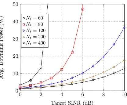
a simple numerical example. We plot the downlink transmit power (obtained by running the ROBF algorithm) as a function of γ for different values of Nt in Figure 1. We consider K= 50UTs per cell and = 0.5 It can be seen that beyond a certain cut off value of the target SINR, the downlink power grows unbounded. This is precisely the value of the target SINR at which the ROBF algorithm becomes infeasible. It can be verified that the cut off value ofγis the one for which the condition in (30) is not satisfied. Finally, note that higher the number of transmit antennas per BS, higher is the cut off value of the target SINR. Once again, this is due to the availability of greater number of spatial degrees of freedom. In this cases whenNt≥2K,any finite target SINR is achievable (note that 2K is the total number of UTs in two cells). The feasibility conditions for the special case of two cell Wyner model was derived in [11] as well.

0 2 4 6 8 10

0 10 20 30 40 50

Target SINR (dB)

Avg.

Do

wnlink

P

ow

er

(W)

Nt= 60

Nt= 80

Nt= 120

Nt= 200

[image:9.612.317.525.55.227.2]

Nt= 400

Fig. 1. Downlink power Vs target SINR forK= 50UTs per cell.

B. Convergence of the Uplink and Downlink SINR

Next we focus on the achieved SINR in the uplink and downlink for the ROBF algorithm. We first start with the analysis of the uplink of the ROBF algorithm. Before we proceed, we make the following observations. Recall that the achieved SINR in the uplink for the ROBF algorithm is given by

ΛUL

i,j(µ) =

µi,j Nt|vˆ

H i,jhi,i,j|

2

P

(n,k)6=(i,j) µn,k

Nt |vˆ H

i,jhi,n,k|2+||vi,jˆ ||22

. (31)

Note that in our notation ΛUL

i,j(µ), we have explicitly

men-tioned the achieved uplink SINR as a function of the pa-rameters of the ROBF algorithm µ (slightly deviating from the notation for the uplink SINR introduced in Section II). Since the uplink receive filter in the ROBF algorithm (13) are minimum mean square error (MMSE) form, the expression for the achieved uplink SINR can be given in alternate form as

ΛUL

i,j(µ) = µi,j

Nt

hH_i,i,j(Σ0iµ+INt)

−1_h

i,i,j (32)

where Σµ_i = P i,j

µi,j Nthi,i,jh

H

i,i,j and Σ

0µ

i = Σ

µ

i −

µi,j Nt hi,i,jh

H

i,i,j.Similarly since the uplink receive filter (8) in

the CBF algorithm are MMSE, the achieved uplink SINR for the CBF algorithm is given by

ΛUL

i,j(λ) = λi,j

Nt

hH_i,i,j(Σ0iλ+INt)

−1_h

i,i,j ∀i, j. (33)

Also, since the CBF algorithm is optimal,

ΛUL

i,j(λ) =γi,j ∀i, j. (34)

Also, recall that the downlink SINR for the ROBF algorithm is given by

ΛDL

i,j(µ) =

|vH i,jhi,i,j|2 P

k6=j|vHi,khi,i,j|2+ P

n6=i,k|vHn,khn,i,j|2+N0 .

(35)

Theorem 3. In the large system regime, the achieved uplink and downlink SINR for the ROBF algorithm converge almost surely to the target SINR γi,j.Mathematically stating

ΛUL

i,j(µ)

a.s.

−−−−−−→

Nt,K→∞

γi,j ∀i, j, (36)

ΛDL

i,j(µ)

a.s.

−−−−−−→

Nt,K→∞

γi,j ∀i, j. (37)

Proof. The details of the proof for the convergence of the achieved uplink SINR (36) can be found in Appendix D.

Next we proceed to the convergence proof for the downlink SINR (37). The proof utilizes the following lemma on the convergence result for the downlink interference terms.

Lemma 4. The downlink interference term corresponding to

the intra-cell and inter-cell interference converge in the large system regime to the following:

X

(n,k)6=(i,j)

|vH_n,khn,i,j|2 X

(n,k)6=(i,j) ¯

δn,kG¯n,i,jG¯n,n,km¯0n Nt

.

(38)

The lemma is proved in Appendix E. We now proceed to the convergence of the downlink SINR. Using Lemma 4 and Lemma 11, it can be concluded that the downlink SINR asymptotically converges to

ΛDL

i,j(µ)

a.s.

−−−−−−→

Nt,K→∞

¯

δi,jσi,i,jG¯i,i,jm¯2i 1

Nt P

(n,k)=(i,j)6 δ¯n,kG¯n,i,jG¯n,n,km¯0n+N0

. (39)

It can be easily verified from (14) that the right hand side of (39) is equal to the target SINR γi,j, thus completing the

proof.

C. Asymptotic optimality of the Uplink and Downlink Power Allocation

We now focus on the optimality of the uplink and downlink power allocation of the ROBF algorithm in the large system regime.

Consider the Lagrangian of the downlink minimization problem in its two forms as in equations (3) and (4). Our proof proceeds by plugging in the solution obtained by the ROBF algorithm (v,µ) into the Lagrangian and examining its properties in the large system regime.

Lemma 5. The following results hold true for the Lagrangian

in the large system limit:

lim Nt,K→∞

L(v,µ) = lim

Nt,K→∞

X

i,j

vH_i,jvi,j, (40)

lim Nt,K→∞

L(v,µ) = lim

Nt,K→∞

X

i,j µi,jN0

Nt

. (41)

.

Proof. Please refer to Appendix F.

We can draw the following inference from the result of Lemma 5.

Corollary 2: The uplink and downlink power allocations

yielded by the ROBF algorithm are equal in the asymptotic limit:

lim

Nt,K→∞

X

i,j

v_i,jHvi,j= lim Nt,K→∞

X

i,j µi,jN0

Nt

. (42)

We know that the uplink power allocation of the CBF algo-rithm satisfies

X

i,j λi,jN0

Nt

= min

w maxλ L(w,λ) (43)

If we show that in the large system regime

lim Nt,K→∞

X

i,j µi,jN0

Nt

= lim

Nt,K→∞

min

w maxλ L(w,λ), (44)

and the duality gap is zero, then this implies that the so-lution provided by the ROBF is optimal in the asymp-totic domain. In other words, the optimal downlink power (which is the solution of the primal problem) is equal to

limNt,K→∞minwmaxλL(w,λ).In order to do so, we prove the following result:

Lemma 6. In the large system regime, the sum of uplink power allocation of the ROBF algorithm converges to the sum of uplink power allocation of the CBF algorithm.

X

i,j µi,j

Nt

X

i,j λi,j

Nt

∀i, j. (45)

Proof. The result is proved in Appendix G.

Consequently, the solution provided by the ROBF algorithm is optimal to limN t,K→∞maxwminλL(w,λ). Also, from the result of Corollary 2, it follows that the downlink power allocation of the ROBF algorithm is also optimal in the large system regime. This concludes the proof.

IV. INCORPORATINGINDIVIDUALBS TRANSMITPOWER CONSTRAINTS

In this section, we consider a practical constraint in MIMO multi-cell systems, namely the individual BS transmit power constraints. Recall that the basic optimization problem consid-ered in this work stated in (2) does not impose this constraint. In what follows, we propose a heuristic extension of the ROBF algorithm to incorporate this constraint.

The optimization problem in (2) along with the individual BS transmit power constraints can be stated as follows:

min wi,j ∀i,j

X

i,j

wi,jHwi,j (46)

s.t. ΛDLi,j ≥γi,j ∀i, j,

X

j

w_i,jHwi,j≤Pi,max ∀i,

wherePi,maxdenotes the peak power of BSi.In what follows,

Algorithm 3 (ROBF with individual BS transmit power constraints). Perform the following steps.

1. Initialize τ= 0, andαi(0)≥0,∀i.

2. Starting from any initial µ0_i,j(τ) > 0 ∀i, j compute the uplink power allocation as µi,j(τ)= limt4 →∞µti,j(τ),

where

µt+1_i,j (τ) = γi,j σi,i,jm¯ti(τ)

∀i, j (47) and m¯t

i(τ) is evaluated as m¯ti(τ)

4

= limp→∞m¯t,pi (τ)

(initializing with anym¯t,0_i (τ)>0,∀i)

¯

mt,p_i (τ) = (48)



 1 Nt

X

n,k

σi,n,kµtn,k(τ)

1 +σi,n,kµt_n,k(τ) ¯m t,p−1(τ) i

+ 1 +αi(τ) 



−1

.

3. Set the receive uplink filter as

ˆ

vi,j(τ) = (49)

1 N0

√

Nt X

n,k

µn,k(τ) Nt

hi,n,khH_i,n,k+ (1 +αi(τ))I−1hi,i,j.

(50)

4. Set the transmit downlink beamforming vectors as

vi,j(τ) = q_¯

δi,j(τ)

Nt vi,jˆ ,where the scaling factors ¯ δi,j(τ)

are calculated as in (14).

5. . Set τ=τ+ 1and update αi(τ+ 1)as

αi(τ+ 1) =



αi(τ) +ζ X

j

vH_i,j(τ)vi,j(τ)−Pi,max



 +

∀i, (51)

where ζ > 0 is a small step size. If αi = 0,∀i ∈ {1, . . . , N}, then terminate. Else if for all i∈ {1, . . . , N}, for whichαi >0 if

X

j

vH_i,j(τ)vi,j(τ)−Pi,max

≤δ, (52)

whereδ >0is a small non zero quantity, then terminate. Else return to Step 2.

We now proceed to provide the main intuition behind this algorithm.

A. ROBF with individual BS transmit power constraints: In-tuition

Consider the optimization problem in (46). In order to solve this problem, we proceed by considering the Lagrangian associated with (46), given by

L0(w,λ,α) =X

i,j

wH_i,jwi,j−X

i,j λi,j

Nt

h|wH_i,jh_i,i,j|2 γi,j

− X

(n,k)6=(i,j)

|wn,khn,i,j|2_−N 0

i

+X

i αi

h X

j

wH_i,jwi,j−Pi,max i

, (53)

whereαiare the Lagrange multipliers associated with the

indi-vidual BS transmit power constraints, andα= [α1, . . . , αN]T

(λi,j has the same interpretation as in (3)). From (3), we can

rewrite (53) as

L0(w,λ,α) =L(w,λ) +X i

αi h X

j

wH_i,jwi,j−Pi,max i

.

(54)

Using duality theory, the solution of the dual problem can be given bymax_α,λminwL0(w,λ,α). Let us denote

g(α) = max

λ minw L

0_(w,λ,α).

Our approach proceeds by showing thatP

jw

H

i,jwi,j−Pi,max

is a sub-gradient direction of the function g(α). Then, the dual problemmaxα[max_λminwL0(w,λ,α)]can be solved by updating the Lagrange multiplierα in the direction of the sub-gradient [24].

In order to do so, consider two vectorsα(1) _andα(2)_.Note

that

g(α(1)) = max

λ minw L

0_(w,λ,α(1)

) =L0(w(1),λ(1),α(1)),

where we use (w(1)_,λ(1)

) to denote the solution to

max_λminwL0(w,λ,α(1)).Similarly, let(w(2),λ(2))denote the solution tomax_λminwL0(w,λ,α(2)).Considerg(α(1)). Firstly, it can be noted that

min

w L

0_(w,λ,α(1)

)≤L0(w(2),λ,α(1)), (55) and hence

max

λ minw L

0_(w,λ,α(1)_)≤max

λ L

0_(w(2)_,λ,α(1)_{). (56)}

Using the definition of g(α(1)) in (56), we conclude that

g(α(1))≤max

λ L

0_(w(2)_,λ,α(1)_{). (57)}

Using (54) in the right hand side of (57), we obtain,

g(α(1))≤

max

λ L(w

(2)_,λ,α(1)_{) +}X

i

α(1)_i h X j

(wi,j(2)) H_w(2)

i,j −Pi,max i

.

(58)

Adding and subtracting the termP iα

(2) i

h P

j(w (2) i,j)

H_w(2)

i,j −

Pi,max i

to the right hand side of (58), and rearranging the terms, we obtain

g(α(1))≤max

λ L

0_(w(2)_,λ,α(2)₎

+X

i

α(1)_i −α(2)_i h X j

(w(2)i,j) H_w(2)

i,j −Pi,max i

=g(α(2)) +X

i

α(1)_i −α(2)_i h X j

(w(2)i,j) H

w_i,j(2)−Pi,max i

(59)

where in (59), we have used the definition ofg(α(2)_).

Conse-quently from (59), it can be concluded thatP j(w

(2) i,j)

definition of a sub-gradient). Therefore, updating the Lagrange multiplier αi in the direction of the sub-gradient solves the

dual problem maxα[max_λminwL0(w,λ,α)] [24]. There-fore,αi must be updated as

αi(τ+ 1) =



αi(τ) +ζ X

j

wH_i,j(τ)wi,j(τ)−Pi,max



 +

∀i, (60)

whereζ >0is a small step size.

Further, for each value of α(τ) one needs to solve the problem max_λminwL0(w,λ,α). This can be solved by repeating the steps of the CBF algorithm for non-zero values of α.

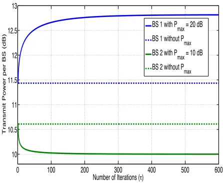
Recall that all the above arguments were made considering the case of finite system dimensions. We now follow the same approach as in the development of ROBF algorithm, i.e., in the large system domain, utilize RMT results to obtain asymptotic approximations of the quantities involved. The ROBF algorithm with per the BS peak power constraints developed in this section is obtained by following this idea. The theoretical analysis of the performance of this algorithm along with the proof of convergence will be a topic of future research. Herein, we resort to the numerical results stated in Section VI in order to show the performance as well as the convergence.

V. IMPACT OFIMPERFECTCSIANDPILOT CONTAMINATION ON THE PERFORMANCE OFROBF

ALGORITHM

In this section, we investigate the impact of CSI estimation errors and pilot contamination on the performance of the ROBF algorithm. Throughout this section, we assume that the slow fading co-efficient (path loss information) can be accurately estimated at the BS (since they remain constant for a long period of time, they are easy to estimate, see for e.g. [25]). Further, for the fast fading co-efficients, we assume reciprocity between uplink and downlink channels, and consider the time division duplexing (TDD) model of channel estimation, i.e., estimation via uplink pilots.

A comprehensive design of the optimal beamforming vec-tors in the presence of CSI estimation errors and pilot con-tamination issue is out of the scope of this paper. Alternately, we take the following approach: First, we assume that the BS treats the CSI estimate as the true CSI and implements the ROBF algorithm directly. In this case, we derive the asymptotic equivalent of the downlink SINR achieved by the ROBF algorithm. Using numerical results, we investigate the impact of CSI estimation errors and pilot contamination on the performance of the ROBF algorithm both in terms of the achieved SINR and downlink power. Then, exploiting the fact that the BS has the accurate knowledge of the slow fading co-efficient, we propose a heuristic adaptation of the ROBF algorithm in the presence of imperfect CSI and pilot contamination named as the modified ROBF (MROBF) algorithm. We show that under the massive MIMO regime, an algorithm in which parameters can be computed based on the

channel statistics (rather than the fast fading CSI) such as the MROBF algorithm is more robust to CSI estimation and pilot contamination effects.

A. CSI Estimation

We now describe the CSI training phase for the estimation of the fast fading co-efficients. Let T be the length of the channel coherence interval, a part of which is dedicated for CSI estimation, and TTr be the number of symbols used for pilots. Therefore, the UTs in every cellitransmitTTrmutually orthogonal pilot symbols to their respective BSs during the training phase. We represent the pilot sequences used by theK UTs in each cell by the matrix√PTrΦ∈

C

TTr×K, (TTr≥K). The pilot sequences are repeated in each cell, hence leading to the issue of pilot contamination. The matrix Φ satisfies

ΦHΦ=IK.

The signal received during the channel training phase de-noted by Yi,Tr∈

C

Nt×K can be written as

Yi,Tr=Hi,iΦT+ X

n6=i Hi,n

ΦT +N, (61)

where Hi,n = [hi,n,1, . . . ,hi,n,K] and N ∈

C

Nt×TTr _with

i.i.d. CN(0,1) elements represents the noise during channel training phase. The MMSE estimate ofhi,n,k givenYi,Trcan be given by [26]

ˆ

hi,n,k =σ_i,n,k0 N X

b=1

hi,b,k+√nTr

PTr

!

, (62)

whereσ_i,n,k0 =σi,n,k

_PN

b=1σi,b,k+_P1_Tr −1

. It can be

veri-fied thathˆi,n,k is distributed as

ˆ

hi,n,k∼ CN



0, σ_i,n,k2 N X

b=1

σi,b,k+ 1 PTr

!−1

. (63)

For notational simplicity, let us denote σˆi,n,k =

σ2 i,n,k

_PN

b=1σi,b,k+_P1_Tr −1

. Note that

ˆ

σi,n,k=σi,n,k0 σi,n,k. (64)

ROBF Algorithm With CSI Estimates

Throughout this subsection, we assume that the BSs assume the CSI estimates to the true channel vector, and implement the ROBF algorithm. Note however that the computation of µi,j and¯δi,j in (11) and (14) do not require the estimates of

the fast fading co-efficient, and hence they can be implemented directly. The uplink receive filter with imperfect CSI denoted byvˆest

i,j can be formulated as

ˆ v_i,jest =

r 1 Nt

Ψ−1

i hi,i,jˆ (65)

where

Ψi=X

n,k µi,k

Nt ˆ

The dowlink beamforming vector denoted byvest

i,jcan be then

computed as

vest_i,j= s

¯ δi,j Nt ˆ

v_i,jest. (67)

We now investigate the achieved SINR in the downlink under the ROBF algorithm with imperfect CSI. The expression for the dowlink SINR can be given as in (35), by replacing

vi,jwithvˆest

i,j.The asymptotic equivalent of the dowlink SINR

can be obtained by analyzing it in the large system regime.

Theorem 4. The achieved SINR in the downlink by the ROBF

algorithm in the presence of imperfect CSI converges almost surely to the right hand side of (71)in the large system regime, where the term Gˆn,n,k is defined as

ˆ

Gn,n,k=

1

1 +ξn,kσˆn,n,km¯estn

and ξi,k = PN

n=1σi,n,kµn,k σi,i,k

.

(68)

Further, m¯est

n can be computed as the solution to the fixed

point equation

¯ mestn =

1 Nt

K X

k=1

ξn,kσˆn,n,k 1 +ξn,kσˆn,n,km¯estn

+ 1 !−1

, (69)

and ( ¯m0_n)est _{can be computed fromm¯}est

n as

( ¯m0_n)est₌ ( ¯mestn )2

1− 1

Nt PK

k=1

(ˆσn,n,kξn,km¯estn)2 (1+ˆσn,n,kξn,km¯estn)2

. (70)

Proof. The proof is provided in Appendix H.

B. Modified ROBF (MROBF) Algorithm

In this subsection, we propose a heuristic adaptation of the ROBF algorithm addressed as Modified ROBF (MROBF) algorithm which is designed to accommodate the effects of imperfect CSI and pilot contamination.

First, note that naive application of the ROBF algorithm may not yield good performance in the presence of imperfect CSI and pilot contamination. The following reasoning provides an intuitive understanding for this: Consider the interference arising from the signal of U Tn,k,(n6=i, k6=j)at the UTi,j

(which does not use the same pilot as UTi,j), i.e., the term

|wn,khn,i,j|2.Following the derivation of Appendix H, it can

be verified that this interference terms converges to

|wn,khn,i,j|2 δ¯n,k Nt

ˆ

σn,n,kGˆ2n,n,k( ¯m

0

n)

est_B

n,k. (75)

Now consider the interference arising from the signal of U Tn,j, (n 6= i) at the UTi,j (which reuses the same pilot

as UTi,j), i.e., the term |wn,jhn,i,j|2. It can be verified that

asymptotically, this interference terms converges to

|wn,jhn,i,j|2_δ¯ n,j

σn,i,jσ0n,n,jGˆn,n,jm¯estn 2

. (76)

We note that the two interference terms are significantly different. In particular, (75) is scaled by a factor of _N1

t, (and for large Nt, this has a very low value). However, the

term in (76) is not scaled. This is due to the fact that the

BS cannot distinguish between the channels of UTi,j and

UTn,j due to the pilot contamination effect. This implies that

naive application of the ROBF algorithm may significantly underestimate the interference arising out of the UTs that reuse the same pilots. The algorithm performance can be enhanced by carefully accounting for these issues. This is indeed the main intuition behind the MROBF algorithm.

In the MROBF algorithm, we consider that the BS does not alter the structure of the beamforming vector, i.e., the BS retains the RZF beamforming vector as in (67). Nevertheless, the performance gain can still be obtained by redesigning the uplink power allocation, and computation of ¯δ. We redesign the uplink power allocation on similar lines as that of the ROBF algorithm.

First note that in the case of perfect CSI, the achieved uplink SINR in the asymptotic limit is given byσi,i,jµi,jm¯i.

Further, the uplink power allocation is chosen to satisfy γi,j=σi,i,jµi,jm¯i, or

µi,j= γi,j σi,i,jm¯i

∀i, j. (77)

We use a similar argument for the computation of the uplink power allocation in the case of imperfect CSI. In order to do so, consider the uplink SINR with uplink receive filter formulated as in (65)

(ΛUL

i,j(µ))est=

µi,j Nt |vˆ

est

i,jhi,i,j|2 P

(n,k)6=(i,j) µn,k

Nt |vˆ

est

i,jhi,n,k|2+||vˆesti,j|| 2 2 .

(78)

Let us examine the uplink SINR in the large system domain. Using the derivation similar to Appendix H, by replacing the individual terms of (78) by their asymptotic equivalents, the uplink SINR in the large system limit can be approximated by (73)3. For convenience, let us denote that denominator of (73) by IUL

asymp. Following the same approach as in (77), we compute the uplink power allocation as the solution to the following set of equations:

µi,j=

γi,jIasympUL

(ˆσi,i,jGˆi,i,jm¯esti )2

∀i, j. (79)

The µi,j that satisfies the set of equations (79) can be

com-puted using the following iterative method: Starting from any initial µ0

i,j >0 ∀i, j the uplink power allocation is given by µi,j

4

= limt→∞µti,j,where

µt+1_i,j = γi,j(I

UL asymp)

t

(ˆσi,i,jGˆti,i,j( ¯mesti )t)2

∀i, j. (80)

In (80), (IUL

asymp)t,Gˆti,i,j and ( ¯mesti )t denote the respective

quantities computed atµt

i,j, ∀i, j.We observe that numerically

that the iterations of (80) converges to the solution of (79) (see numerical results in Section VI).

Finally, ¯δ can be computed as a solution to the following linear equations

¯

δ=∆−1γ (81)

(ΛDL

i,j(µ))est

¯

δi,j(ˆσi,i,jGˆi,i,jm¯esti )2

PN n=1 n6=i ¯ δn,j

σn,i,jσ0n,n,jGˆn,n,jm¯estn 2

+ 1

Nt PN

n=1 PK

k=1 k6=j ¯

δn,kσˆn,n,kGˆ2n,n,k( ¯m0n)estBn,k

, (71)

where

Bn,k =σn,i,j+ ˆσn,n,j(ξn,jσn,i,jσ0n,n,jGˆn,n,jm¯nest)2−2µn,j(σn,i,jσn,n,j)0 2Gˆn,n,jm¯estn . (72) µi,j(ˆσi,i,jGˆi,i,jm¯esti )2

PN n=1 n6=iµn,j

σi,i,jσ0i,n,jGˆi,i,jm¯esti 2

+ 1

Nt PN

n=1 PK

k=1 k6=j

µn,kσˆi,i,jGˆ2i,i,j( ¯m0i)estBn,k0 + ˆσi,i,jGˆ2i,i,j( ¯m0i)est

, (73)

where

B_n,k0 =σi,n,k+ ˆσi,i,k(ξi,kσi,n,kσ0i,i,kGˆi,i,km¯esti )

2_−2µi,k(σ

i,n,kσ0i,i,k) 2_Gˆ

[image:14.612.50.267.235.399.2]

i,i,km¯esti . (74)

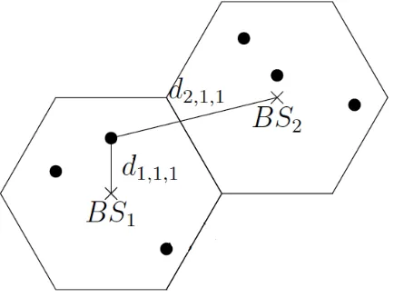
Fig. 2. Hexagonal cellular network consisting of2cells.

where the matrix ∆∈

_C

N K×N K is defined as

∆=



 

∆1,1 . . . ∆1,N

..

. . .. ...

∆N,1 . . . ∆N,N





 (82)

where each submatrix ∆i,j∈

C

K×K is given by

∆i,n_j,k =4      

    

(ˆσi,i,jGˆi,i,jm¯iest)2, n=i, k=j

−σn,i,jσ0n,n,jGˆn,n,jm¯estn 2

, n6=i, k=j

−1 Ntˆσn,n,k

ˆ G2

n,n,k( ¯m0n)estBn,k, n=i, k6=j

andn6=i, k6=j. (83)

VI. NUMERICALRESULTS

In this section, we present some numerical results to demon-strate the performance of the ROBF algorithm in a massive MIMO setting.

We consider a hexagonal cellular system consisting of 2

cells as shown in Figure 2. We use the distance dependent path loss model in which the path loss from BS ito UTj,k is

given by

σi,j,k= d0

di,j,kβ ,

wheredi,j,k represents the distance between BSito UTj,k. β

represents the path loss exponent which is taken to be3.6in all

the simulation scenarios.d0represents the channel attenuation

at reference point and is taken to10−3.53_{.Location of the UTs}

are obtained by generating uniform random numbers inside each hexagonal cell. The distance dmin ≤ di,j,k ≤ dmax,

where dmin and dmax represent the minimum and the

max-imum distance between the UTs to the BSs of their respective cells. In our simulation,dmin= 20m anddmax={500,1000}

m depending on the distance between the two BSs. The noise power is taken to be−104dBm over the operating bandwidth. All numerical results are plotted by varying the positions of the UTs inside the cell over500 iterations.

First, we examine the performance of the ROBF algorithm in satisfying the UT SINR constraints. Accordingly, we plot the variation of the uplink and downlink SINR (averaged across the UTs) as a function of the number of antennas per BS for1000channel realizations in Figure 3. Herein,K= 50

UTs per cell and target SINR is3dB per UT. The horizontal line represents the target SINR which is 3 dB. The bubbles represent the average achieved SINR values (averaged over the channel realizations), and the vertical lines around this bubble represent the variation of the achieved downlink SINR around the average value. It can be observed that even for moderate number of antennas, e.g. 60antennas per BS (comparable to the number of UTs), the target SINR constraints are satisfied for almost every channel realization (since the fluctuations are small). This implies that the ROBF algorithm nearly optimal under this setting in terms of satisfying the SINR constraints.

Next, we investigate the downlink power of the ROBF algorithm and compare it with the CBF algorithm and ZF beamforming4 (denoted by qPZF

i,jw

ZF

i,j, where wZFi,j is unit

norm vector). Note that our simulation setting, the BS per-forms ZF beamforming to null the interference UTs in both the cells (and not merely the UTs in its own cells). After nulling the interference, BS performs appropriate power allocation in

50 100 150 200 250 300 350 400 2.5

3 3.5

No. of Anternnas per BS N_t

Achieved SINR (Donwlink) − dB

Target SINR

[image:15.612.68.534.65.249.2]

Mean value of achieved SINR Standard deviation

Fig. 3. Fluctuations of the downlink SINR (ROBF algorithm) around the target value.K= 25UTs per cell and target SINR =3dB per UT.

50 100 150 200 250

5 10 15 20 25 30 35 40 45

No. of Antennas per BS (N_t)

Dowlink power per UT (dBm)

ZFBF CBF ROBF

Fig. 4. Comparison of downlink power per UT as a function of the number of antennas per BS.K = 25UTs per cell and target rate =3bits/s/Hz

(log(1 +γi,j)) per UT.

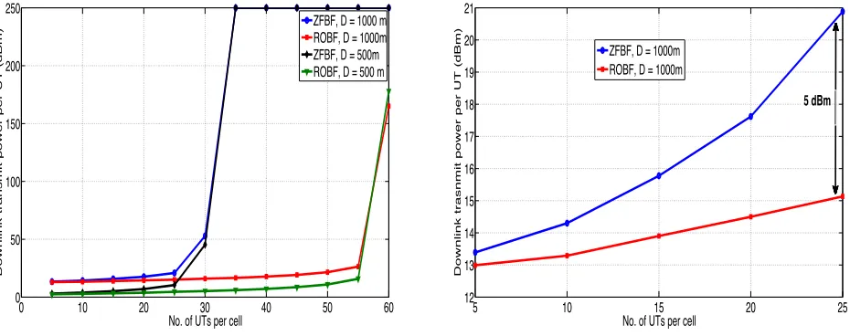
0 10 20 30 40 50 60

0 50 100 150 200 250

No. of UTs per cell

Downlink transmit power per UT (dBm)

ZFBF, D = 1000 m ROBF, D = 1000m ZFBF, D = 500m ROBF, D = 500 m

Fig. 5. Comparison of downlink power per UT as a function of the number of UTs per cell. Nt = 60antennas/ BS and target rate = 3 bits/s/Hz

(log(1 +γi,j)) per UT.Drepresents the distance between the two BSs.

5 10 15 20 25

12 13 14 15 16 17 18 19 20 21

No. of UTs per cell

Downlink trasnmit power per UT (dBm)

ZFBF, D = 1000m ROBF, D = 1000m

5 dBm

Fig. 6. Comparison of downlink power per UT as a function of theK. Settings identical to Figure 5.

order to meet the target SINR constraint of the UTs

P_i,jZF= γi,jN0

|hi,i,jwi,jZF|2 .

We plot the downlink power per UT (i.e. Sum downlink power_K ) as a function of the number of antennas per BS in Figure 4. Herein, K = 25 UTs per cell and target rate = 3 bits/s/Hz (log(1 + γi,j)) per UT. The following conclusions can be drawn. First, the downlink power expended by ROBF very closely matches that of CBF, indicating that the ROBF is nearly optimal in terms of minimizing the downlink power as well. Next, it can be seen that for moderate number of antennas per BS, e.g.

50−100antennas, ROBF provides substantial power gains as compared to ZF beamforming. This result highlights the gains obtained by optimizing the power allocation (as compared to naively nulling out interference to all the UTs in the system). When Nt is very large, the scaling of _N1_t starts to play a

dominant role, and ROBF ceases to provide substantial gains over ZF.

Finally, we examine the efficacy of ROBF algorithm in terms of its ability to support greater number of UTs per cell. This is accomplished by fixing the number of antennas per BS to 60, and plotting the downlink power as a function of the number of UTs per cell in Figure 5. It can be seen that beyond a certain number of UTs, the downlink power corresponding to the ZF beamforming becomes unbounded. In fact, this happens at K = 30 UTs per cell (note that Nt = 2K at this point

[image:15.612.71.536.299.483.2]