http://wrap.warwick.ac.uk
Original citation:
Loomes, Graham, Professor of economics and Pogrebna, Ganna (2015) Do preference reversals disappear when we allow for probabilistic choice? Working Paper. Coventry: Warwick Manufacturing Group. WMG Service Systems Research Group Working Paper Series (Number 08/15).
Permanent WRAP url:
http://wrap.warwick.ac.uk/70154
Copyright and reuse:
The Warwick Research Archive Portal (WRAP) makes this work by researchers of the University of Warwick available open access under the following conditions. Copyright © and all moral rights to the version of the paper presented here belong to the individual author(s) and/or other copyright owners. To the extent reasonable and practicable the material made available in WRAP has been checked for eligibility before being made available.
Copies of full items can be used for personal research or study, educational, or not-for-profit purposes without prior permission or charge. Provided that the authors, title and full bibliographic details are credited, a hyperlink and/or URL is given for the original metadata page and the content is not changed in any way.
A note on versions:
The version presented here is a working paper or pre-print that may be later published elsewhere. If a published version is known of, the above WRAP url will contain details on finding it.
WMG Service Systems Research Group
Working Paper Series
Do Preference Reversals Disappear When
We Allow for Probabilistic Choice?
_____________________________________________________________________
Graham Loomes
Ganna Pogrebna
ISSN: 2049-‐4297
About WMG Service Systems Group
The Service Systems research group at WMG works in collaboration with large organisations such as GlaxoSmithKline, Rolls-‐Royce, BAE Systems, IBM, Ministry of Defence as well as with SMEs researching into value constellations, new business models and value-‐creating service systems of people, product, service and technology.
The group conducts research that is capable of solving real problems in practice (ie. how and what do do), while also understanding theoretical abstractions from research (ie. why) so that the knowledge results in high-‐level publications necessary for its transfer across sector and industry. This approach ensures that the knowledge we create is relevant, impactful and grounded in research.
In particular, we pursue the knowledge of service systems for value co-‐creation that is replicable, scalable and transferable so that we can address some of the most difficult challenges faced by businesses, markets and society.
Research Streams
The WMG Service Systems research group conducts research that is capable of solving real problems in practice, and also to create theoretical abstractions from or research that is relevant and applicable across sector and industry, so that the impact of our research is substantial.
The group currently conducts research under six broad themes:
• Contextualisation • Dematerialisation • Service Design
• Value and Business Models • Visualisation
• Viable Service Systems and Transformation
WMG Service Systems Research Group Working Paper Series
Issue number: 08/15
Do Preference Reversals Disappear When We Allow for
Probabilistic Choice
?
Graham Loomes
Warwick Business School, University of Warwick, Gibbet Hill Road, Coventry, CV4 7AL, UK
E-‐mail: [email protected]
Ganna Pogrebna
Service Systems Group, Warwick Manufacturing Group, University of Warwick, Gibbet Hill Road, Coventry CV4 7AL, UK
E-‐mail: [email protected]
Acknowledgement: Graham Loomes acknowledges support from the UK Economic and
Social Research Council (grants RES-‐051-‐27-‐0248 and ES/K002201/1) and from the Leverhulme Trust ‘Value’ Programme RP2012-‐V-‐022. Ganna Pogrebna acknowledges financial support from the Leverhulme Trust under the Early Career Fellowship scheme. Both authors are grateful to the attendees at the NIBS 2015 Conference in Nottingham for useful comments and suggestions.
If you wish to cite this paper, please use the following reference:
Loomes G & Pogrebna G (2015) Do Preference Reversals Disappear When We Allow for
Do Preference Reversals Disappear When We Allow for
Probabilistic Choice?
1. Introduction
More than three decades ago, Grether and Plott (1979) drew economists’ attention to an unsettling regularity reported by experimental psychologists (Lichtenstein and Slovic, 1971; Lindman, 1971). The regularity in question – the ‘preference reversal phenomenon’ – took the following form. Two lotteries were constructed: a ‘$-‐bet’ which offered a relatively high payoff with a probability well below 0.5; and a ‘P-‐bet’ which offered a considerably higher probability of a more modest payoff. Participants in the experiment were asked to do three things: to place a certainty equivalent value1 upon the $-‐bet; to place a certainty equivalent value upon the P-‐ bet; and to make a straight choice between the two. Most conventional decision theories suppose that an individual who prefers one bet to the other will pick the preferred option when offered a choice between the two and will also place a higher certainty equivalent value on whichever option he/she prefers. However, Lichtenstein and Slovic reported that a substantial proportion of their experimental participants flouted this expectation by choosing the P-‐bet while placing a strictly higher value on the $-‐bet. The opposite ‘anomaly’ – choosing the $-‐bet while placing a higher value on the P-‐bet – was rarely observed. It is this asymmetry which constitutes the classic preference reversal (PR) pattern.
Grether and Plott (1979) had initially supposed that this phenomenon would disappear – or at least, be greatly attenuated – if stronger incentives and stricter experimental controls were deployed. But in fact the phenomenon persisted, and many other experiments since that time have found this classic PR pattern of behaviour to be easy to replicate and quite difficult to eliminate without considerable effort and/or supplementary mechanisms – see the survey by Seidl (2002).
At the level of modelling, this phenomenon would appear to present a fundamental challenge to general theories that assume transitivity. At the level of practical application, it raises concerns about the use of stated values as a basis for guiding public policy: if such patterns also occur in the domain of (say)
1 Most often, this value has been elicited as a ‘reservation selling price’ – that is, the individual is given
environmental goods, there is a danger that using stated willingness-‐to-‐pay in cost-‐ benefit analysis might lead to priority being given to projects that would not be chosen if citizens were in a position to express choices or rankings directly. For reasons of both theory and policy, therefore, it is important to gain a better understanding of what this phenomenon really represents in terms of the structure of human preferences and/or the validity of different procedures for eliciting those preferences.
This paper aims to contribute to a better understanding of those issues. The next section discusses in more detail the main competing explanations of PR and some of the evidence for and against the different accounts. That discussion raises issues about the noisiness or imprecision of many people’s responses, so in Section 3 we outline a (deliberately broad) framework of probabilistic preferences within which our inquiry will be conducted. In Section 4 we report two substantial experiments. The data generated by these experiments strongly suggest that for pairs of bets typical of the PR literature, most people’s preferences exhibit some degree of stochastic variability, but their ‘core’ preferences mostly conform with the probabilistic formulation of transitivity known as Weak Stochastic Transitivity. Put another way, when certainty equivalent values are inferred from repeated binary choices, the classic PR phenomenon largely disappears and the reversals that remain are relatively few in number and small in magnitude. By contrast, when certainty equivalent values are elicited more directly via a standard incentive-‐compatible mechanism, the same individuals display a very strong PR pattern of the usual kind. Our results broadly support the conclusions drawn by Tversky et al. (1990) and Bostic
et al. (1990), although we find ‘overvaluation’ of all bets rather than the mix of overvaluation and undervaluation that those studies report.
It is not possible to reconcile the data with conventional deterministic models – even those that permit some level of preference reversal (e.g., Loomes and Sugden, 1983). So in Section 5 we explore the data we have generated to see if we can shed further light on the disparities between choice and valuation and we discuss whether we can account for them in terms of a model of probabilistic choice known as Decision Field Theory (Busemeyer and Townsend, 1993). It turns out that this model – at least, as applied by Johnson and Busemeyer (2005) – cannot readily accommodate our data, so in the final section we discuss some possible directions for future theoretical development and some implications for applied research.
2. Different Possible Explanations of the Classic PR Pattern
2.1 Intransitive Preferences
One possible hypothesis is that the classic PR pattern reflects preferences that allow systematic intransitivity over binary choices. Let us write the $-‐bet as $, write the P-‐ bet as P, and denote strict preference by ≻. Suppose we can find some sure amount of money M such that an individual has the preferences $ ≻M, M ≻P and P ≻$: that is, suppose that for this particular {$, P, M} triple she has intransitive preferences.
If asked to give her certainty equivalent for the $-‐bet, CE($), she will state some CE($) > M; and if asked to give her certainty equivalent for the P-‐bet, she will state CE(P) < M. Hence when asked to give the two valuations and also make a direct choice between $ and P, as in standard PR experiments, she will report CE($) > CE(P) and P ≻$, thereby exhibiting the classic PR pattern. In so doing, there is no bias or error in her responses: she is accurately reporting her preferences, but happens to have preferences that, in this case, do not conform with transitivity. Although many decision theories take transitivity as axiomatic, not all theories do so: for example, Regret Theory (Bell, 1982, Loomes and Sugden, 1982, 1983) allows preferences of the kind that would produce the classic PR pattern for at least some {$, P} pairs.2
Of course, if this intransitivity explanation is correct, it should be possible to find evidence of the $ ≻M, M ≻P and P ≻$ cycles that would underpin the classic PR pattern. A paper by Loomes et al. (1991) reported an experiment where choice cycles in this classic direction did indeed outnumber those in the opposite direction, seemingly to a significant extent. However, only a minority of all responses were cyclical and it was suggested by Sopher and Gigliotti (1993) that the patterns reported by Loomes et al. (1991) could possibly have arisen purely as a result of noise/error. This is an issue to which we shall return below.
2.2 Procedural Biases
A rather different kind of explanation of the PR phenomenon was offered by Lichtenstein and Slovic (1971). Other variants have been suggested since, but what they have in common is the idea that people may not have highly articulated underlying preferences which are always accurately and consistently expressed in response to every task, but rather may to some extent construct their responses according to the nature of the task presented to them and may therefore be systematically influenced by certain features of the different procedures used.
2 An intuitive explanation of how Regret Theory works in this context is as follows. An individual who
So, for example, when asked to give a certainty equivalent – that is, when asked to give a response in terms of a sum of money – it may be that individuals are (subconsciously) prompted to pay extra attention to the money dimension and underweight the probability information. Perhaps – especially when the task is framed as selling – they initially ‘anchor’ on the bet’s most desirable payoff and then arrive at their valuation by adjusting down from that payoff to allow for the possibility that some lower payoff may result; but they do not adjust sufficiently and hence tend to generate a higher certainty equivalent for the bet with the higher payoff, namely the $-‐bet. By contrast, when asked to make a straight choice between $ and P, it may be that more attention is paid to the chances of winning at least something; and since the P-‐bet offers a bigger chance of winning something than the $-‐bet, this serves to increase the likelihood that the P-‐bet will be chosen. In short, the weight given to different dimensions may be influenced by the nature of the elicitation procedure, resulting in a systematic disparity between the preference inferred from direct choice and the preference inferred from the two separate valuations.
Tversky et al. (1990) conducted some experiments intended to try to diagnose the causes of preference reversals, both for risky options and for intertemporal decisions. With respect to $-‐bets and P-‐bets (which they relabelled L and H), they concluded that the phenomenon was primarily due to what they regarded as overvaluing the L ($) bet, partly due to undervaluing the H (P) bet, with perhaps 5%-‐ 10% of the effect due to intransitivity.
However, there are reasons to be cautious about the basis for this diagnosis. One reservation concerns the mechanism used to elicit the values of the bets. Participants were told that at the end of any session involving real payoffs, a pair of lotteries would be selected at random. There was then a 50% chance that a participant would be paid on the basis of playing out whichever option he had picked in the direct choice task; and there was a 50% chance that he would instead play out whichever option he had placed a higher value upon. While Tversky et al. (1990, p.207) argued that this “ordinal payoff scheme” avoided some of the objections that had been made against the standard Becker-‐DeGroot-‐Marschak (1964) mechanism, it had the disadvantage that it was no longer necessary to identify the true indifference value for each bet, since it was only the ordering of the values rather than their precise magnitudes that mattered. In the absence of a mechanism designed to give accurate magnitudes, it is arguably unsafe to make statements about ‘overvaluing’ or ‘undervaluing’ on the basis of ordinal responses.
intransitive over some range). So an experiment which uses a small set of options involving a limited number of pre-‐set parameters may well hit upon the critical region for some individuals but might miss it for others with different underlying preferences, even though these people might display intransitivity in other (unexplored) triples.
The studies conducted by Bostic et al. (1990) tried to address the latter issue by eliciting choices via two different iterative procedures (while using the Becker-‐ DeGroot-‐Marschak mechanism to incentivise valuations elicited in a more conventional way). Bostic et al. (1990) found that their first iterative choice experiment reduced the prevalence of cycles compared with classic PR patterns but did not eliminate the asymmetries between cycles for two {$, P} pairs out of four. Their second experiment, using a more concealed iterative choice procedure3, seemed to reduce the significance of asymmetrical cycles even further, but had a rather small sample of just 21 respondents.
2.3 Imprecise or Probabilistic Preferences
There is a third kind of explanation that focuses on the possible importance of the imprecise or probabilistic nature of many people’s preferences.
At the less structured end of the spectrum of such accounts, MacCrimmon and Smith (1986) suggested that the classic PR pattern could be explained in terms of the $-‐bet allowing a much wider range of valuation responses that do not violate first-‐ order stochastic dominance than the range allowed by the P-‐bet, so that individuals who were unsure about their precise certainty equivalent could more easily pick higher values for the $-‐bet than for the P-‐bet without being obviously wrong. If both bets have (roughly) the same minimum payoff (small negative amounts in the early experiments, often zero in more recent experiments), there is more scope for giving higher values for the $-‐bet than for the P-‐bet but less scope for giving lower values, which would be sufficient to produce the classic asymmetry.
MacCrimmon and Smith (1986) noted that if the same reasoning were applied to the elicitation of probability equivalents, the opposite asymmetry might be expected.4 Butler and Loomes (2007) conducted an experiment to explore these
3 Bostic et al. (1990, p.204) expressed some concern that in their first experiment, the iterative
procedure may have become so transparent that it affected respondents’ answers by putting them into a valuation frame of mind. Experimental economists might also fear that a transparent procedure could encourage strategic answers intended to influence the options offered subsequently. The second procedure used by Bostic et al. (1990), was less transparent and therefore less vulnerable to those concerns.
4 Instead of asking for a sure amount of money that the individual considers exactly as desirable as a
possibilities and found some evidence that people’s uncertainty about their own preferences varied in ways consistent with MacCrimmon and Smith’s conjectures.
At the more structured end of the spectrum, Blavatskyy (2009) has proposed a model which embeds a deterministic Expected Utility Theory (EUT) core in a particular stochastic specification and has shown how some asymmetry in the classic PR direction might result. The detail of this approach is different from that used by Sopher and Gigliotti (1993) mentioned above, but the general proposition is similar: namely, that if an individual’s expressed preferences involve some stochastic component, that component, although itself random, may interact with core preferences in such a way as to produce seemingly systematic departures from standard presumptions. Under certain conditions, this model can even accommodate what Fishburn (1988, pp. 45-‐46) called ‘strong’ reversals.5
Johnson and Busemeyer (2005) explored the possibility that Busemeyer and Townsend’s (1993) Decision Field Theory might provide an explanation. The key idea is that individuals arrive at a valuation response after a cognitive process of iteration between each bet and some sequence of sure amounts. They hypothesised that the starting point of such a process typically involved higher sure amounts when $-‐bets were being valued than when P-‐bets were being processed and that it was this that tended to produce CE($) > CE(P) even when P ≻$ in a direct comparison.
In Section 5, we will discuss this and the various other possible explanations outlined above. First, however, we set the scene for our experiments.
3. A Broad Probabilistic Choice Framework
It has often been observed that when the same individual is presented with exactly the same tasks framed in exactly the same way on more than one occasion within a fairly short period of time, he/she may answer somewhat differently in at least some of those repetitions. An early manifestation of such behaviour was reported by Mosteller and Nogee (1951), who encountered variability of this kind when they presented respondents with a variety of choices, each repeated multiple times over a period of several weeks. For example, one series of decisions asked respondents either to accept or refuse a gamble that involved a ⅓ chance of losing 5c and a ⅔ chance of winning X, where X took a number of different values ranging from 5c through 7c, 9c, 10c, 11c, 12c to 16c. Over the course of the experiment, each
range between 0 and 0.7 without violating dominance while q is constrained by dominance to lie between 0 and 0.3, there is more scope to give a higher probability equivalent for the P-bet while perhaps choosing the $-bet in the direct choice between the two.
5 A ‘strong’ reversal is a case where the P-bet is chosen even though the stated certainty equivalent for
level of X was presented to each respondent on up to 14 independent occasions. Mosteller and Nogee (1951, Figure 2) depicted a respondent who never accepted the gamble when X was 5c or 7c and always played it when X was 16c, but for intermediate values his acceptance rate lay between 7% and 93%, increasing monotonically with X. Such variability (although often less neatly monotonic) was typical of the other participants in their study – and has been observed in many subsequent studies involving repeated choices.
Over the years, such variability has been formally modelled in a number of ways – see Luce and Suppes (1965) for an early review and Rieskamp et al. (2006) for a more recent one. However, as Stott (2006) and Blavatskyy and Pogrebna (2010) have shown, different assumptions about the way in which the stochastic component is specified can produce quite different estimates of underlying parameters. So in order to avoid becoming embroiled in debates about the sensitivity of our results to particular functional forms, our strategy in this paper is to try to investigate the issues raised above within a framework of probabilistic choice so general that it encompasses a very broad range of more specific stochastic models and relies on a bare minimum of assumptions.
Consider a case where an individual is presented with a number of choices between some lottery B and a series of increasing sure amounts denoted by Aj. If these choices could be presented on a number of different occasions and under circumstances where an individual makes each choice independently of every other one – in the sense of not remembering previous choices and therefore making each new choice afresh – then we might model an individual’s underlying preferences as a probability distribution.
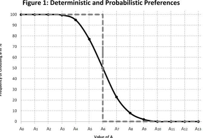
Figure 1 shows two possible distributions. The dashed line shows the deterministic preferences of an individual who is indifferent between B and a sure amount A6: for all j < 6, she always chooses B and for all j > 6 she never chooses B, while for j = 6, all probability mixes of A and B are equally good.
Figure 1: Deterministic and Probabilistic Preferences
Using Pr(A≻B) to denote the probability of choosing A from the pair {A, B}, we shall refer to cases where Pr(A≻B) = Pr(B≻A) = 0.5 as cases of stochastic indifference (SI). This is the stochastic analogue of the notion of certainty equivalence in deterministic theories. In the example shown in Figure 1, the SI point is at A6.
The curve in Figure 1 is no more than an illustration and we make no strong claims about its shape. We have drawn it as sigmoid because that seems to fit many intuitions and datasets. We leave open the question of symmetry: some model specifications may imply symmetry while others may suggest particular kinds of asymmetry, but such detail is not necessary for our purposes. All we wish to convey in Figure 1 is the distinction between deterministic and probabilistic choice and the broad proposition that models of probabilistic choice allow there to be some range between the point where B is always chosen and the point where B is never chosen6, and that between those two points the probability of choosing B falls monotonically as A becomes unambiguously better.
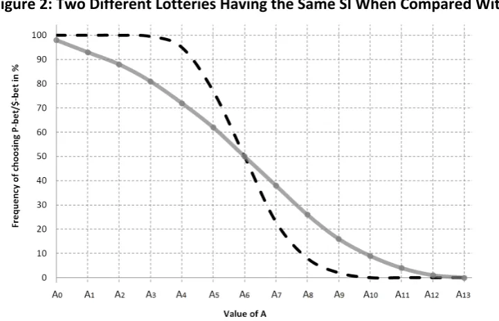
Now let us consider two different lotteries represented on the same diagram. In Figure 2, let the dashed curve represent the distribution for a particular P-‐bet while the solid curve shows the distribution for a particular $-‐bet, where Pr($≻P) = Pr(P ≻$) = 0.5 and where both of these bets are stochastically indifferent to the sure amount A6. Thus we have constructed a case which is consistent with Weak Stochastic Transitivity (WST), which, for any triple {X, Y, Z}, requires that if Pr(X≻Y) ≥ 0.5 and Pr(Y≻Z) ≥ 0.5, then Pr(X≻Z) ≥ 0.5.
6 Here we are abstracting from what have come to be called ‘trembles’ – that is, cases where a
[image:12.595.130.466.76.304.2]However, even when WST holds, patterns of choice over specific pairs located away from the SI points may exhibit what looks like systematic disparities. To see this, suppose that we have a sample of 100 individuals whose preferences are each as in Figure 2. Instead of asking them to choose between pairs involving A6, suppose we set the sure amount at A8.
Each participant is assumed to make each choice as if on the basis of independent draws from the underlying distributions in Figure 2. Most will give responses that are consistent with transitive orderings over {$, P, A8}, but there will be some sets of choices that are intransitive, either in the direction consistent with the classic PR or else in the opposite direction.
The cycle corresponding with the classic PR pattern is $≻A8, A8≻P and P≻$. From Figure 2 we read off Pr($≻A8) = 0.27 and Pr(A8≻P) = 0.93. Combining these probabilities with Pr(P≻$) = 0.5 and assuming independent draws, the product of these probabilities is 0.12555, so that on average we should expect to observe 12 or 13 members of our sample exhibiting the cycle consistent with the classic PR pattern. The opposite cycle involves $≻P, P≻A8 and A8≻$, for which the probabilities are 0.5, 0.07 and 0.73, giving a product of 0.02555, so that we should expect 2 or 3 people to report this pattern. Even if we round the first number down and round the second number up, we have a 12:3 ratio between the two cycles. If we were to apply the standard binomial test, in effect, testing the null hypothesis that both types of cycle are equally likely, we should reject that hypothesis at the 5% level. Thus we can see how probabilistic preferences which respect transitivity at the core may nevertheless give the appearance of systematic asymmetries in responses to a particular set of predetermined options.
[image:13.595.125.486.500.732.2]How might we depict probabilistic preferences which do not respect WST? Suppose we could find a {$, P} pair such that Pr(P≻$) > 0.5 while at the same time the underlying probability distributions for each bet against different sure sums is as in Figure 3.
Figure 3: $-‐bet SI > P-‐bet SI
As in Figure 2, the dashed curve represents the {Aj ,P} relationship while the solid curve shows {Aj ,$}. Here the SI for the $-‐bet is A7 while the SI for the P-‐bet is A6. So if we set the sure sum between A6 and A7 – half way between, for example, which we denote by A* – then we should see WST violated because at that level of A, Pr($≻A*) = 0.58 while Pr(A*≻P) = 0.65, which should imply Pr($≻P) ≥ 0.5, whereas we have a {$, P} pair such that Pr($≻P) < 0.5.
Notice, however, that such a violation of WST is only observable for A between A6 and A7. If we were to set the sure sum at anything less than A6, both Pr($≻A) and Pr(P≻A) > 0.5 so that no violation of WST can be detected; and likewise when the sure sum is greater than A7 so that both of those probabilities are less than 0.5. Even if underlying preferences are as shown in Figure 3, the scope for demonstrating violations of WST in the direction consistent with the classic PR pattern is limited. It is easy to see that even if all individuals have preferences with the potential to violate WST, they may have different SIs such that any particular pre-‐set value of A will only fall into the critical range for a subset of them.
[image:14.595.124.493.155.407.2]amounts and see how the ordering of these SIs compares with the modal choice between them. Denoting the SI for the S-‐bet as SI($) and the SI for the P-‐bet as SI(P), the possibilities are as follows. If SI(P) ≥ SI($) and Pr(P≻$) ≥ 0.5, or if SI($) ≥ SI(P) and Pr($≻P) ≥ 0.5, the individual conforms with WST. However, if SI($) > SI(P) but Pr(P≻ $) > 0.5, the individual violates WST in the direction consistent with the classic PR pattern, whereas if SI(P) > SI($) but Pr($≻P) > 0.5, the violation of WST is in the opposite direction. The experimental design described in Section 4 seeks to obtain the required estimates of SI($), SI(P) and Pr($≻P).
4. Experimental Design
4.1 General Principles
In principle, we should like to take various $-‐bets and P-‐bets and, for each bet, identify the range of sure sums that cover the distance between the highest sure sum which is (almost) never preferred to the bet and the lowest sure sum which is (almost) always preferred to the bet; and within that range, to have enough pairs each repeated enough times (ideally, with each choice independent of all earlier presentations of the same pair) to provide a good estimate of the curve in question and a reasonably precise estimate of the SI point.
Bearing in mind that any sample is likely to involve some degree of heterogeneity between individuals, in an ideal world one might like to have different sure sums £0.50 or £1 apart covering most of the range between the upper and lower P-‐bet payoffs, with perhaps 10 repetitions of each {Aj, $} and {Aj, P} pair. One might also like to have comparable numbers of repetitions between each {$, P} pair. However, such a design could easily entail four or five hundred choices for a single {$, P} pair, which, when interspersed among a similar number of ‘distractor’ choices, would be a daunting prospect for potential participants and might compromise the quality of the data.
On the basis of our own and colleagues’ experience and a pilot study, we judged that we should produce a design using no more than 200-‐300 questions in total, with a number of these questions involving tasks other than binary choices in order to try to provide some variety and extra interest for participants.7 The net
7 When respondents are presented with a large number of tasks, there is necessarily a judgment to be
result was a design that included up to 36 different pairs, with each pair presented as binary choices (BCs) on four occasions during the experimental session and with each of these presentations being separated from one another by a number of other pairs also presented in random order.
We shall set out in subsequent subsections the particular parameters used and we shall present evidence to demonstrate that the data showed reasonable sensitivity to variations in those parameters. But first we address a possible concern about whether four repetitions are sufficient for our purposes. Certainly, if our objective were to produce a reasonably tight-‐fitting curve for each individual for each lottery, four observations per pair would not be sufficient. However, for the purpose of covering the range within which nearly everyone’s SI is located and thereby getting an estimate of each SI, we believe that our design is adequate.
To explain how we analysed the data, consider Figure 4, which shows on the horizontal axis the different sure values that A might take, while the vertical axis measures the numbers of times some bet is chosen in any four repeated pairings with the same A.
The black dots represent the responses of an individual with probabilistic preferences. When asked to choose between a $-‐bet and nine sure sums, each presented on four separated occasions, she always chooses the $-‐bet when the alternative is £4 or £5 and never chooses it when A offers £11 or £12 for sure. But for sums from £6 to £10, she chooses each alternative on at least one occasion – and is even observed to choose the $-‐bet more often (twice) when the sure amount is £8 than when the sure amount is £7. Of course, such seeming inconsistency is likely to occur simply by chance if the individual is behaving as if sampling just a few times from an underlying probability distribution of the kind described in Section 3.
[image:16.595.134.456.519.715.2]Her choices between a P-‐bet and the same set of sure amounts are shown by the grey diamonds. She always chooses the P-‐bet when the sure alternative is £7 or less and she never chooses the bet when the sure sum is £8 or more. Her behaviour here is indistinguishable from what we might expect of someone with deterministic preferences whose CE lies between £7 and £8 and if we have to give a best estimate of that CE, we have no reason to do other than take the midpoint of £7.50. The same applies to our best estimate for the SI of an individual with probabilistic preferences who reports those choices.
Where does this individual’s sure-‐sum SI for the $-‐bet stand in relation to her SI for the P-‐bet? There is more variability in the $-‐bet responses, but if we had to judge which of the two bets had the greater SI in terms of sure sums, we should have to conclude on this evidence that there is no significant difference between them: for £4, £5, £11 and £12 they make the same choices throughout; when the sure sum is £6 or £7, the P-‐bet is chosen four more times; but when the sure sum is £8, £9 or £10, the P-‐bet is chosen four fewer times. With the small number of discrete choice observations involved, sophisticated econometric estimation may offer little more than we can achieve by simply counting the number of times each bet is chosen out of the total of 36 decisions. In the above example, each bet is chosen 16 times against the same set of sure amounts, mapping to an SI value of £7.50.
Had the individual in the above example chosen (say) the P-‐bet more often, it would have suggested a higher SI value for that bet. For example, suppose that the she had made the same choices as above except that she had chosen the P-‐bet twice in the {£8, P} pair. On that basis, an SI of £8 would seem to be the best estimate. In other words, choosing the bet 18 times in total maps to an SI value of £8. More generally, when the range of A options is as shown in Figure 4 and when each {Aj, bet} pair is presented on four separated occasions, we estimate SI(bet) = £3.5 + 0.25B, where 0 < B < 36 is the total number of times a particular bet is chosen.8
We shall therefore conduct our analysis of SI points in terms of the numbers of times the bet in question is chosen from any given range of alternatives. There will of course be some sampling error for such a measure, but our sample sizes in conjunction with the within-‐subject nature of the analysis will still allow us to draw a number of conclusions.
4.2 Experiment 1
Experiment 1 examined the relationship between direct choice between $ and P and the ordering of the SI values inferred from repeated choices involving the
same set of sure amounts. In short, it was designed to look for evidence about conformity with – or else systematic departure from – WST when such bets are involved. The conventional wisdom, as expressed in Rieskamp et al. (2006, p. 648) is that violations of WST are quite rare and tend to occur only in “fairly unusual” circumstances, so that “the principle of weak stochastic transitivity should generally be retained as a bound of rationality”. Unfortunately, a number of the experiments they cite could be argued to have involved too few repetitions over too narrow a range to provide a really strong foundation for this conclusion. Our experiment had the drawback that it was constructed around just one {$, P} pair, but its strength was that it involved multiple repetitions and therefore gave a reasonable chance of detecting violations of WST, if there were any to be detected.
In our pair, what we shall call the focal $-‐bet offered a 0.3 chance of £40 (otherwise 0) and our focal P-‐bet offered a 0.7 chance of £15 (otherwise 0). Each bet was displayed as shown in the upper panel of Figure 5 when participants were being asked to make a straight choice between the two bets and as in the lower panel of Figure 5 when the alternative was a sure sum of money – in this case, the choice is between our focal $-‐bet and £11 for sure. The text accompanying each kind of choice is also reproduced.
We opted for this way of displaying alternatives in order to try to strike a compromise between the ‘decision by description’ and ‘decision by experience’ approaches. A growing literature9 suggests that when people form an estimate of probabilities on the basis of some sampling experience, they may behave differently from when the probabilities are merely stated in decimal or percentage form without the opportunity for participants to get some ‘feel’ for them. The large number of decisions in our design made it impossible to ask people to learn the probabilities for each choice by sampling, but by showing the distributions of balls that give positive or zero payoffs in a format that allowed probabilities to be easily seen and compared, we hoped to provide a visual proxy for experience by showing exactly what each option would involve in terms of the 20 balls that would be put into a bag when one of the choices came to be played out for real.
The focal $-‐bet was presented on four separated occasions in choices with nine different sure integer amounts from £4 to £12, providing a total of 36 BCs. The focal P-‐bet was offered against the same nine sure sums, giving another 36 choices. We also had nine pairs where the focal $-‐bet was fixed while the alternative bet’s probability of £15 varied from 0.5 to 0.9 with increments of 0.05, each presented on four separated occasions; and another nine pairs where the focal P-‐bet was held constant while the alternative bet’s probability of £40 varied from 0.15 to 0.55 with increments of 0.05. Thus we have a total of 4 x 9 x 4 = 144 BCs. For each individual,
then, we can estimate a certainty equivalent SI for the focal $-‐bet and a certainty equivalent SI for the focal P-‐bet, and we can compare the ordering of these SIs with the frequency of choice from a total of eight separated presentations of the focal {$, P} pair.
This experiment involved 101 participants through the online recruitment system of the Decision Research at Warwick (DR@W) Group in the University of Warwick. Each participant received an invitation with detailed instructions together with a link to the online experiment. Participants were invited to complete the online experiment in their own time by a specified deadline. Each invited participant was assigned a unique ID number which was automatically copied as a password to the experimental interface. This insured that (a) only invited participants could take part in the experiment and (b) none of participants could take part more than once. The experiment was computerised using the Experimental Toolbox (EXPERT) online platform.10
Besides the 144 BC questions described above, there were a further 36 questions presented in the form of four 9-‐row choice lists: these took the total of incentivised lottery-‐based tasks to 180, with these being mixed up and spread over sections 1, 3 and 5 of the experiment. Sections 2 and 4 consisted of quite different tasks involving 2 x 6 hypothetical questions of the type used in the Domain Specific Risk Attitude (DoSpeRT) procedure (Blais and Weber, 2006). These two sections were included as ‘distractor’ tasks for our participants, providing greater separation between repetitions of the incentivised questions. They play no part in our analysis.
Figure 5: Examples of Displays Used in Binary Choices
(a) Binary choice between the focal $-‐bet and the focal P-‐bet
[image:19.595.92.520.638.714.2]
(b) Binary choice between the focal $-‐bet and an amount of money for certain
The incentive mechanism was as follows. On the date of the specified deadline, 100 participants were selected at random from all participants who completed the experiment on time.11 These participants were invited to the DR@W experimental laboratory for individual scheduled appointments. One of the 180 incentive-‐linked questions was picked at random and independently for each participant and was played out for real money. There was no show-‐up fee and the instructions made it clear that the participant’s entire payment depended on how her decision played out in the one randomly-‐selected question.
If the participant had chosen some sure amount of money, she would simply receive that sum. If she had chosen a lottery, she would see an opaque bag being filled with the numbers of red and black balls (actually, coloured marbles) specified in the question. She then picked a marble at random and was paid (or not) accordingly.
This incentive mechanism was described to all participants in the instructions. Participants also received a practice question and had an opportunity to e-‐mail the experimental team in case they were not clear about the instructions. On average, it took each participant 30-‐40 minutes to complete the online experiment. Each individual appointment in the DR@W laboratory lasted between 3 and 5 minutes. The average payoff in the experiment was approximately £12.
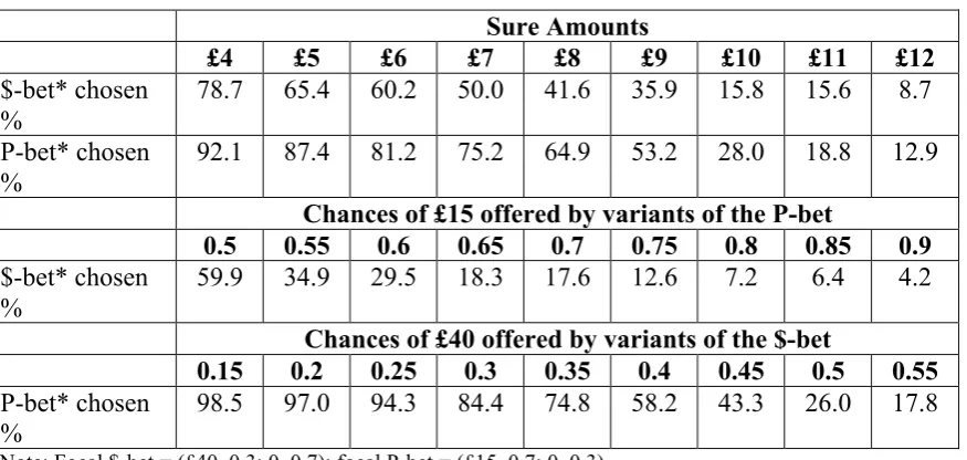
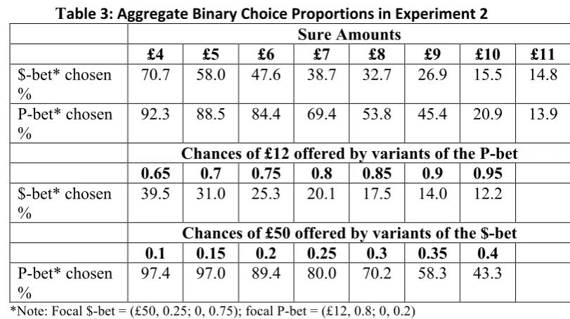
We begin by presenting various aggregate patterns of response, so that readers can form some view about the extent to which the data showed broad regularities of the kind most models might entail. Table 1 shows how the likelihoods
11 This experiment was in fact one of two being conducted in parallel using the same general format of
of choosing the fixed lotteries changed as the alternatives became progressively better. In all cases, the proportions were sensitive in the expected directions to variations in parameters.
Table 1: Aggregate Binary Choice Proportions in Experiment 1
Sure Amounts
£4 £5 £6 £7 £8 £9 £10 £11 £12
$-bet* chosen %
78.7 65.4 60.2 50.0 41.6 35.9 15.8 15.6 8.7
P-bet* chosen %
92.1 87.4 81.2 75.2 64.9 53.2 28.0 18.8 12.9
Chances of £15 offered by variants of the P-bet
0.5 0.55 0.6 0.65 0.7 0.75 0.8 0.85 0.9
$-bet* chosen %
59.9 34.9 29.5 18.3 17.6 12.6 7.2 6.4 4.2
Chances of £40 offered by variants of the $-bet
0.15 0.2 0.25 0.3 0.35 0.4 0.45 0.5 0.55
P-bet* chosen %
98.5 97.0 94.3 84.4 74.8 58.2 43.3 26.0 17.8
*Note: Focal $-bet = (£40, 0.3; 0, 0.7); focal P-bet = (£15, 0.7; 0, 0.3)
At this aggregate level, the central tendencies look broadly consistent with transitivity. Overall, the P-‐bet was chosen in just over 83% of the direct choices between the focal $-‐bet and the focal P-‐bet. At the same time, on the basis of the choices between each bet and the different sure amounts, the sample median valuation of P was a little over £9 while the sample median valuation of $ was £7. At this level of analysis, the majority choice was compatible with the ordering of median values.
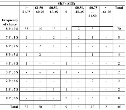
However, the usual PR asymmetry is an individual-‐level phenomenon. So Table 2 assigns individuals to cells according to the relationship between the frequency with which they chose $ or P in the direct choice between them (shown in the rows) and the ordering over the two bets inferred from the difference between their SI certainty equivalents, with the SI differences being grouped into seven column categories.
[image:21.595.102.540.177.385.2]Table 2: Choice and SI Valuation Differences Inferred from BCs in Experiment 1
SI(P)–SI($) ≥
£1.75
£1.50 - £0.75
£0.50, £0.25 0
–£0.50, –£0.25
–£0.75 - – £1.50
≤ –£1.75
Total
Frequency of choice
8 P ; 0 $ 33 15 13 4 2 3 - 70
7 P ; 1 $ 2 1 2 - 2 1 - 8
6 P ; 2 $ - 2 1 - - - - 3
5 P ; 3 $ 1 2 - - - 1 - 4
4 P ; 4 $ 1 - - 1 - - - 2
3 P ; 5 $ - - - 1 - - 1 2
2 P ; 6 $ - - - 2 - 2
1 P ; 7 $ - - 1 1 - - - 2
0 P ; 8 $ - - - 2 - 5 1 8
Total 37 20 17 9 4 12 2 101
[image:22.595.89.514.109.480.2]However, Experiment 1 was built around just one particular {$, P} pair and it could be objected that the results might not generalise to other pairs. Moreover, Experiment 1 focused exclusively on choice-‐based tasks and did not at the same time elicit valuations in a more direct way, using the kind of incentive mechanism more commonly used in conjunction with selling/buying prices in traditional preference reversal experiments. So in Experiment 2 we used slightly more extreme bets that might be regarded as (even) more typical of many PR experiments and we added a conventional valuation task to the other formats used in Experiment 1 so that we could make direct within-‐person comparisons.
4.3 Experiment 2
Many features of this experiment were the same as in Experiment 1 in terms of the numbers of binary choices and the incentive system for those choices. The two key differences between this experiment and the previous one were as follows. First, the new focal $-‐bet offered a 0.25 chance of £50 (otherwise 0) and the new focal P-‐ bet offered a 0.8 chance of £12 – that is, the two bets were a little further apart in terms of probabilities and payoffs and expected values than the pair in the first experiment. Second, we dropped the DoSpeRT questions and replaced them in Sections 2 and 4 with 20 direct valuation (DV) tasks linked to the kind of incentive mechanism often used, due to Becker, DeGroot and Marschak (1964). Those 20 DV tasks involved five different lotteries, each valued on two separated occasions in Section 2, and again twice each in Section 4, thus giving four separated valuations for each lottery. Figure 6 shows an example of a typical DV task – in this case, for the focal P-‐bet in the current experiment.
Two of those five lotteries were the $-‐bet and P-‐bet which are focal to this experiment. Two others were the $-‐bet and P-‐bet used in Experiment 1. The fifth lottery was one used in the ‘independence’ experiment run in parallel with Experiment 1, as referred to in footnote 11 above.
By embedding the DV tasks in among many BCs involving the same or similar bets and sure amounts, our intention was to give participants every opportunity to be consistent across the two types of task. We also tried to formulate the valuation task to be as much like a choice task as we could, avoiding any reference to ‘price’ or to selling or buying. That is, we were consciously attempting to reduce any framing effects so as to examine the question of whether a valuation task per se was treated differently than a series of binary choices.
Confirm and Proceed and then either valued a fresh lottery or else, at the end of each series of ten valuations, moved on to another series of BCs.
So, for example, an individual might move the slider, steadily increasing the amounts shown in the boxes until (say) the left-‐hand box displayed £7.50 and the right-‐hand box displayed £7.60. The respondent would thereby be stating that he would rather play the lottery than get £7.50 and would rather get £7.60 than play the lottery.
Figure 6: Example of Display Used in Experiment 2 Direct Valuation
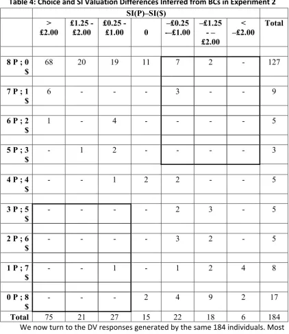
A total of 184 participants from the University of Warwick completed all of the BC and DV questions. On this basis, for each participant we could identify from the BC responses:
• The individual’s SI certainty equivalent for the $-‐bet;12 • The individual’s SI certainty equivalent for the P-‐bet; • The distribution of 8 straight choices between $ and P.
[image:24.595.92.544.480.614.2]