Analysis and computation for Bayesian inverse problems

(1)

warwick.ac.uk/lib-publications

A Thesis Submitted for the Degree of PhD at the University of Warwick

Permanent WRAP URL:

http://wrap.warwick.ac.uk/86136

Copyright and reuse:

This thesis is made available online and is protected by original copyright.

Please scroll down to view the document itself.

Please refer to the repository record for this item for information to help you to cite it.

Our policy information is available from the repository home page.

(2)

M A

O

D

C

S

Analysis and Computation for Bayesian

Inverse Problems

by

Matthew M. Dunlop

Thesis

Submitted for the degree of

Doctor of Philosophy

Mathematics Institute

The University of Warwick

(3)

Acknowledgments

I would first like to thank my supervisors Andrew Stuart and Marco Iglesias for their help, guidance and support, without which this thesis would not have been possible. They have introduced me to a fascinating, rich field of mathematics that regularly provides new and interesting problems. I’d also like to thank my examiners Carola-Bibiane Sch¨onlieb and Marie-Therese Wolfram for taking the time to read this thesis, and for their many helpful comments. Thank you also to everybody involved with the EQUIP programme, for the support and stimulating discussions.

Next, I thank everyone I’ve shared an office with over the past four years, providing a welcoming environment for questions and discussion. In particular, I’d like to thank Graham Hobbs, Ben Lees and David O’Connor for the many helpful chats over lunches, tea, coffee and otherwise.

I would also like to thank the Engineering and Physical Sciences Research Council (EPSRC) for funding my position in MASDOC, and the University of Warwick Mathematics department for their hospitality.

(7)

Declarations

The work described in this thesis is the author’s own, conducted under the super-vision of Andrew Stuart (University of Warwick) and Marco Iglesias (University of Nottingham), except where otherwise stated. More specifically:

(i) Chapter 1 is an introduction containing a literature review and outline of the thesis content.

(ii) Chapter 2 is work done in collaboration with Andrew Stuart, and has been submitted for publication [44]. Changes were made on the advice of two anony-mous referees.

(iii) Chapter 3 is work done in collaboration with Andrew Stuart, and has been submitted for publication [45].

(iv) Chapter 4 is work done in collaboration with Andrew Stuart and Marco Igle-sias, and has been submitted for publication [43]. The numerical simulations presented in section 4.4.2 are due to Marco Iglesias.

(8)

Abstract

Many inverse problems involve the estimation of a high dimensional quantity, such as a function, from noisy indirect measurements. These problems have received much study from both classical and statistical directions, with each approach having its own advantages and disadvantages. In this thesis we focus on the Bayesian approach, in which all uncertainty is modelled probabilistically.

Recently the Bayesian approach to inversion has been developed in function space. Much of the existing work in the area has been focused on the case when the prior distribution produces samples which are continuous functions, however it is of in-terest, both in terms of applications and mathematically, to consider cases when these samples are discontinuous. Natural applications are those in which we wish to infer the shape and locations of interfaces between different materials, such as in tomography.

(9)

Chapter 1 Introduction

In section 1.1 we describe what is meant by an inverse problem, and provide some examples of challenges associated with the solution of such problems. In subsection 1.1.1 we give an overview of some classical approaches to overcome these challenges, first in the linear finite-dimensional case, and then more general cases. In subsection 1.1.2 we then describe the modern Bayesian approach to inverse problems, where the solution is now a probability measure, rather than a state or set of states. In section 1.2 an outline of the content of the thesis is given, with a brief overview of the results in each chapter.

1.1 Overview

(10)

oil well to be constructed. In a medical context, data could arise via X-ray measure-ments or some other tomographic method. Decisions made based on the analysis of this data could include how to or whether to intervene surgically.

A common theme in many of these applications is that the data is not complete – it cannot uniquely determine the unknown quantity. In this case, the problem could be represented in terms of an equation of the form

y=_G(u) (1.1.1)

where G : (X,k · kX) → (Y,k · kY) is a (often non-linear, non-invertible) mapping

between two Banach spaces, termed theforward map. In this equationu_∈X repre-sents the unknown input to be determined from a number of (frequently noisy and indirect) measurements, and y ∈ Y represents the observed data. In applications, the forward map is typically formed by composing a forward model with an obser-vation map. The forward model could for example involve the solution of a partial differential equation related to a physical system, given some inputu, and the ob-servation map could take this solution to its valuesyat a discrete set of observation points.

Another theme is that there may be significant noise on measurements, meaning that even if there is enough data, it may not be consistent with both the physical model and itself. In this case the observations may, for example, take the form

y=G(u) +η (1.1.2)

where η is a realization of some random noise. Physically this could correspond to measurement instruments having only finite precision, or might be included to account for differences between the computer model and physical reality [78]. Often this noise will be assumed Gaussian, though other distributions are not uncommon depending on the context [59, 103].

(11)

1.1.1 Classical Approaches to Inversion

In order to remove or reduce the effects of ill-posedness from an inverse problem, one could attempt to modify the problem in an appropriate manner, or modify what is meant by a solution to the problem. Well-studied techniques for doing so include variational regularization approaches, truncation of spectral decomposi-tions, definition of notions of quasisoludecomposi-tions, and contruction of dynamical systems with suitable ergodic properties. Such techniques have been considered for a large variety of problems, including inverse spectral problems [46, 110, 140], inverse ob-stacle scattering [32, 81, 118], tomography [29, 58, 120], image processing and decon-volution [87, 88, 129], and seismic inversion [111, 113, 127]. The structure in these problems, such as the regularity of the forward map, the dimension (or effective dimension) of the input and the data, and the amplitude of the noise, can have a strong effect on what technique is appropriate and how effectively the input can be recovered.

In order to illustrate the technologies available, we will first outline least-squares based methods for linear forward maps on finite dimensional spaces, before dis-cussing methods for more general maps.

LetXandY be finite dimensional Hilbert spaces, and let the forward mapA:X_→ Y be linear so that the data y now arises via

y=Au.

Assuming thatA is not invertible, an alternative way of characterizing solutions to this problem is in the least-squares sense. Denote by Φ :X →R the least-squares

functional associated with this problem,

Φ(v) := 1

2kAv−yk

2

Y,

and denote by _{U ⊆} X the set of minimizers of Φ. Since Φ is smooth and convex, we can characterize _U by for example checking first- and second-order optimality constraints. That isv∈ U if and only if Φ0(v) = 0 and Φ00(v) is non-negative definite. We calculate

Φ0(v) =A∗Av−A∗y, Φ00(v) =A∗A

and deduce thatv_{∈ U} if and only if it satisfies the normal equations:

(12)

However, unless A∗_A _{is invertible, this system will admit an infinity of solutions.}

Consider the case whenX=Rn and Y =Rm are Euclidean spaces andA∈Rm×n.

Suppose first that m_≥ nso that the system is overdetermined, and rank(A) =n. Then all of the singular values ofA are strictly positive, hence the same is true of the eigenvalues ofA∗A: there exists a unique solution to (1.1.3). If instead we have

m < n and rank(A) = m, then rank(A∗_A_{) =} _{m < n} _{and so there exist infinitely}

many solutions to (1.1.3). In general, we have infinitely many solutions whenever rank(A)<min{m, n}, so that rank(A∗A) = rank(A) < n. In all cases there exists at least one solution – this could also be seen by noting that Φ is continuous and coercive.

Even when we are in the case that there exists a unique solution, the behavior of this solution with respect to perturbations in the datay may be poor. If A admits the singular value decompositionA =UΣV∗_{, then it can be checked that the solution}

is given by

u=VΣ−1U∗y (1.1.4)

where Σ−1 _∈ Rn×m is given by (Σ−1)ii = 1/Σii for i = 1, . . . , n and (Σ−1)ij = 0

otherwise. Hence if any of the singular values Σii of A are close to zero, small

changes iny can lead to large changes in u.

Typically there will be an infinite number of solutions to (1.1.3), and so it may be preferable to pick out a particular solutionu with certain properties. For example, it may be of interest to to choose the solutionu0∈ U whose norm inX is minimal,

that is,

u0 = argmin

v∈U

1 2kvk

2

X. (1.1.5)

A relaxation of this approach is to introduce a regularization parameterλ >0, and instead seek minimizers of the perturbed least-squares functionalJλ :X→R,

Jλ(v) := Φ(v) +

λ

2kvk

2

X.

(13)

the corresponding normal equations are now given by

(A∗A+λI)v=A∗y,

and (A∗_A₊_λI_{) is always positive-definite and hence invertible. Moreover, we have}

thatuλ →u0 ∈ U asλ→0, whereu0 is as defined by (1.1.5).

Returning to the Euclidean case X = Rn, Y = Rm discussed earlier, it can be

verified that instead of (1.1.4), the solution uλ to the perturbed problem may be

represented as

uλ =VΣ−_λ1U∗y

where Σ−_λ1_∈Rn×m is given by

(Σ−_λ1)ii=

Σii

Σ2_ii+λ

fori= 1, . . . , n and (Σ−_λ1)ij = 0 otherwise. Hence by choosing λsufficiently large,

the effect of small singular values of A on data-sensitivity of the solution can be controlled. This is one sense in which the perturbation of the objective functional can be thought of as a regularization of the problem.

Alternatively, returning to the general case, if one takes a subspace (E,_{k · k}E)

em-bedded inX, it may be of interest to penalize the norm inE rather than the norm inX in order to promote certain properties of the solution [48], an approach com-monly referred to as Tikhonov-Phillips regularization. Additionally, the problem of making the optimal choice of regularization parameter λ has received signifi-cant interest, since it is not always appropriate or efficient to consider the limit

λ_→0 [47, 54, 125].

Such an approach can also be used when the data is noisy, that is

y=Au+η.

If the noise is known to be Gaussian distributed with zero mean and covariance Γ, i.e. η _∼ N(0,Γ), then it is natural to consider the weighted least-squares func-tional

Φ(v) := 1

2kAv−yk

2 Γ:=

1 2kΓ

−1

2(Av−y)k2

Y

(14)

of noise.

Other misfit functions and regularization terms have received much study [40,48,80]. In general, the spacesX, Y will be infinite-dimensional Banach spaces and G:X→

Y will not necessarily be linear. With data given by (1.1.1) or (1.1.2) it still makes sense to formulate the problem variationally, so that solutions can be defined to be minimizers of the functionalJ :X →R∪ {∞},

J(v) = Φ(v) +λR(v). (1.1.6)

Here, Φ :X→Ragain represents the model-data misfit, and nowR:X →R∪{∞}

is a general (typically convex) regularization term. These methods are often referred to asTikhonov-type orgeneralized Tikhonov methods. WhenX andY are function spaces, possible choices for Φ andR may include, for example,

Φ(v) = 1

pkG(v)−yk

p Lp,

R(v) = 1

qkBvk

q

Lq or R(v) =

1 2kvk

2

E or R(v) =

1

2kvkTV,

for some p, q _≥ 1, some non-negative operator B, and some (E,_{k · k}E) compactly

embedded in X. B may for example be a differential operator, in which case the regularity of minimizers can be controlled, or a multiple of the identity, in which case their amplitudes can be controlled. As in the finite-dimensional linear case, the choice of the squared E-norm as a regularization term is known as Tikhonov-Phillips regularization [48]. The choice of the total variation (TV) regularization term is often used when the unknown function is piecewise continuous; the TV norm penalizes the surface area of the discontinuity set, and so over-fitting of data can be avoided [114].

Note that due to the non-linearity in _G, the minimizers of J in the case p =q = 2 do not satisfy a linear system as before. This presents issues both from analytical and computational perspectives. Another issue is that in general Φ will not be convex, and so more work is needed to obtain existence of minimizers ofJ. In these cases there may exist multiple local minima which are not the global minimum. These local minima may however be of interest in order to get a fuller picture of the solution of the problem, instead of just looking at the global minimum.

(15)

the regularization termR subject to the condition that the misfit Φ is not too large. Specifically, one can look for solutions in the set

argmin

v∈X

R(v)

Φ(v)≤δ

where δ is approximately the size of the data error, that is δ ≈ Φ(u†), and u† is the true state that generates the data. Note that the calculation of δ does not in general require knowledge ofu†, only of the model: if for example Φ is given by the least-squares functional, then we have that

Φ(u†) = 1 2kηk

2

Y

and so we may use the distributional properties ofη to estimate δ.

Finally one could consider a combination of the Tikhonov-type and residual meth-ods. Denote byuλ the solution to (1.1.6) using regularization parameterλ. We can

look for the choice ofλ such that Φ(uλ) = Φ(u†). This is a root finding problem,

and is known as Morozov’s discrepancy principle [33].

1.1.2 The Bayesian Approach to Inversion

Probability can be used to account for incomplete data and noise on the measure-ments. The Bayesian approach treats all unknowns as random variables, and so inference about these random variables then allows us to perform inference on the system itself. Bayes’ formula tells us quantitatively how to marry data with prior beliefs to produce theposterior distribution. This is a probability measure which, in the context of inverse problems, will typically be defined on an infinite-dimensional Banach space. Quantities of interest, for example posterior mean, variance and modes, can then be studied under this distribution. Since the solution to the prob-lem is now a probability measure rather than a single state, we are able to quantify any uncertainty arising in these quantities via integration. Moreover, whilst the classical approaches discussed in the previous subsection were somewhat ad hoc, the Bayesian approach provides a constructive approach to regularization, especially through the connection with MAP estimators elaborated below.

The following are the main components in the Bayesian approach:

(16)

We typically denote this byµ0.

2. Likelihood. A function_Lrepresenting how likely data is to have arisen from a given stateu, i.e. the conditional density ofygiven u. We will typically write this in the form

L(y;u) = exp(₋Φ(u;y)).

3. Posterior distribution. A probability measure onX that arises by combining the prior distribution and likelihood using Bayes’ theorem, representing the conditional distribution ofu given the datay. Denoting this measure by µy_,

it is given by

dµy

dµ0

(u) = 1

Z(y)exp(−Φ(u;y)) (1.1.7) whereZ(y) is the normalization constant.

The posterior distributionµy _{is the solution to the Bayesian inverse problem. Once}

we have this, many questions may arise. For example:

(i) How sensitive is the posterior distribution to perturbations of the data? How about the choice of prior distribution?

(ii) If the forward model isn’t perfect, either mathematically or computationally, what effect will this have?

(iii) How can we sample the posterior numerically, and ensure that sampling effi-ciency does not decay as any approximation meshes are refined?

Such questions are addressed in generality in the lecture notes [39] and the references therein. The sensitivity in (i) and (ii) is typically characterized with respect to the Hellinger metric, which leads to error bounds on expectations of different quantities. Question (iii) is addressed by formulating any sampling algorithms on function space

before any discretization, and showing such algorithms are well-defined.

The Bayesian and classical approaches to inversion may be related via the modes of the posterior distribution, termed MAP estimators. If the posterior distributionµy

admits a Lebesgue density, so that it can be written dµy

du (u)∝exp(−J(u)),

then a MAP estimator forµy _{is defined as a maximizer of this density, or equivalenty}

(17)

variational problem, and the choice of prior distribution is akin to the choice of regularization term in the classical approaches discussed earlier. In general there will not exist a Lebesgue density, however the definition of MAP estimators may be extended to this case. In [38] the authors provide a definition involving ratios of measures of balls of diminishing size, in such a way that it agrees with the standard definition when Lebesgue densities exist. Later on we will see a direct relation between MAP estimation and Tikhonov-Phillips regularized minimization, in the case of Gaussian observations and Gaussian priors, proved in [38].

An overview of the area of statistical, and in particular, Bayesian approaches to inverse problems is provided in the text [75], with a strong focus on cases where Lebesgue densities exist. This is often the case if, for example, the forward map is assumed to be defined on a finite element space rather than an infinite dimensional function space. Many computational issues are also discussed therein, related to ap-proximation of integrals of quantities of interest against the posterior distribution. Markov Chain Monte Carlo (MCMC) methods are commonly used in practice, which produce Markov chains whose states, in stationarity, are drawn from the posterior. These states can then be used to approximate integrals via Monte Carlo approxi-mation. MCMC techniques typically require many evaluations of the likelihood to produce accurate approximations of quantities of interest, due to strong correlations between states. One is often therefore interested in how the posterior distribution could be approximated by sampling simpler distributions, such as a Gaussians, since these may be sampled much more cheaply. Possible approximations that have been considered previously include linearization around the MAP [113], randomized max-imum likelihood [112] and ensemble Kalman filtering [1]. A comparison of these approximations in the context of reservoir simulation is provided in [70].

As in the classical case, the situation when the forward map is linear and defined on finite dimensional spaces can be easier to analyze. Let X, Y be finite dimensional Hilbert spaces and let A:X _→ Y denote the forward map. Take a Gaussian prior

µ0 =N(m0,C0) onu, and assume the noise has a Gaussian distributionη∼N(0,Γ).

Then the posterior is again Gaussian, with meanmand covariance_Cgiven by

C= (A∗Γ−1A+_C0)−1, m=_C(A∗Γ−1y+_C₀−1m0).

(18)

than the prior covariance. If the Fisher information is zero, then any data will be uninformative and the posterior equals the prior. On the other hand, as the size of the Fisher information increases, the posterior variance contracts to zero and the posterior mean converges to the true state that generates the data – this is an example of what is termedposterior consistency [30].

Note that the posterior mean is the unique minimizer of the functional

J(v) = 1

2kAv−yk

2 Γ+

1 2kC

−1

2

0 (v−m0)k2X (1.1.8)

and thus there exists a clear link between classical and Bayesian approaches in the linear Gaussian case. Note also that the posterior Lebesgue density is given by

dµy

du (u)∝exp(−J(u)).

This is maximized wheneverJ is minimized, and so the posterior mean is the unique MAP estimator in this case.

The non-linear non-parametric case can be significantly more difficult to analyze. The lecture notes [39] provide an overview of many areas associated with such prob-lems. Posterior consistency results have been obtained in, for example, [4, 5, 38]. It is this setting that is considered throughout the majority of this thesis. One of the main obstacles with the non-parametric approach is the the lack of existence of a Lebesgue measure on the space X, and so absolute continuity between mea-sures becomes a much more central property. In particular, the absolute continuity (1.1.7) of the posterior with respect to the prior means that any almost sure prop-erties of the prior, such as sample regularity, are also almost sure propprop-erties of the posterior.

In [38] the authors provide the following result regarding MAP estimators in the non-linear non-parametric case. Suppose that the priorµ0 is chosen to be Gaussian1 with associated Cameron-Martin space (E,_k·kE) compactly embedded in (X,k·kX).

Then under appropriate conditions on the forward map G, MAP estimators are shown to be equivalent to minimizers of the functional J : X _→ R∪ {∞} given

by

J(v) = 1

2kG(v)−yk

2 Γ+

1

2kv−m0k

2

E

for v −m0 ∈ E, and infinity otherwise. A link between Bayesian and classical

inversion techniques is hence again evident. Note also that in the case thatX is a

1

(19)

separable Hilbert space and the prior covariance_C0is strictly positive, the

Cameron-Martin space takes the form (E,k · kE) = (C₀1/2X,kC

−1/2

0 · kX), and so J takes the

same form as (1.1.8) whenever it is finite. In general, however, minimizers ofJ will not coincide with the posterior mean due to the non-linearity of_G.

1.2 Outline of the Thesis

The recent development of Bayesian inversion on function space described in the previous section is focused predominantly on cases where fields sampled from the prior distribution (and hence posterior distribution) are almost surely continuous. There are however many applications where the unknown field is expected, or known a priori, to be discontinuous. This includes for example applications in subsur-face and medical imaging, where intersubsur-faces between different materials correspond to jump discontinuities [20, 85, 113], and deconvolution of piecewise constant sig-nals [28, 64, 121]. In this thesis we develop the mathematically challenging case of reconstruction of piecewise continuous fields from noisy non-direct measurements. The recovery of these fields could be thought of as the joint recovery of the values the fields take in the regions where they are continuous, and the shape of the inter-faces between these regions. We can consider different ways to parametrize both of these.

In what follows the forward map will often take the following form. Let X, Y, V

denote three Banach spaces, and letZ denote a function space. Define the following three maps between these spaces:

• F : X → Z is a construction map, which maps a (typically infinite) set of parameters to a function. This allows for construction of functions with a certain structure, such as being piecewise continuous and/or positive.

• K :Z _→V is a forward model. This is typically a non-linear map involving the solution of a partial differential equation.

• O :V _→ Y is an observation map, which for example maps a function to its values at a discrete set of points.

(20)

1.2.1 Chapter 2 – MAP Estimators for Piecewise Constant Inver-sion

In this chapter we consider the case where the interfaces can be parametrized finite dimensionally, but the fields infinite dimensionally. As such, the parameter spaceX

takes the formX = Λ_×W where Λ_⊆Rk denotes the set of geometric parameters

defining the interfaces, and the space W = C(D;RN) contains the fields between

these interfaces. Such a setup was considered using a Bayesian approach in [71]. A natural application would be in a reservoir model where we are trying to infer the subsurface structure: it may be known that there is a fault occurring in the geology, but the location and size of this fault, along with the permeabilities of the different media, may be unknown. We place a compactly supported prior with continuous Lebesgue density on the geometric parameters, and a Gaussian prior on the fields, so that the prior permeability is piecewise Gaussian with random interfaces. We look at MAP estimation for this problem, i.e. determination of posterior modes, as has been considered in a function space context in [38]. Since X is infinite dimensional, the posterior distribution does not admit a Lebesgue density that can be maximized; we instead use the definition of mode provided in for example [38], involving maximizing ratios of measures of balls of diminishing size. Similarly to [38] the MAP estimators can be characterized as minimizers of a particular functional on the product space of fields and geometric parameters. Numerically solving this minimization problem we observe that, when a non-trivial geometric model is used, the posterior distribution arising can be highly multi-modal. Such observations are confirmed by the behavior of MCMC simulations.

The work in this chapter is in collaboration with my PhD supervisor Andrew Stuart (University of Warwick), and is contained in [44]. This work complements that of [71] and [38] by extending the existence and well-posedness theory from [71] to more general forward maps than groundwater flow, and by analyzing the problem of MAP estimation for more general priors than the Gaussians considered in [38].

1.2.2 Chapter 3 – The Bayesian Formulation of EIT

(21)

Dirichlet-to-Neumann (DtN) or Neumann-to-Dirichlet (NtD) map. More precisely, ifD⊆Rd and g∈H1/2(∂D) is given, letu∈H1(D) solve

 



−∇ ·(σ_∇u) = 0 inD u=g on∂D.

Then does the DtN mapping Λσ :H1/2(∂D)→H−1/2(∂D) given by

g_7→σ_∇u_·ν,

whereν is the outward unit normal to the boundary∂D, determine the coefficientσ

inD? An associated, more ill-posed inverse problem is to ask whether noisy partial knowledge of the NtD map (Λσ)−1 :H−1/2(D)→H1/2(D) allows for determination

ofσ. Much work has been done in this area, for example [6,77,106,132]. An overview of results in the DtN case is given in [20].

A physically realistic PDE model for the problem, of interest in medical imaging, was introduced in [128]. In this chapter we provide a rigorous Bayesian formulation of this EIT problem in an infinite dimensional setting, leading to well-posedness in the Hellinger metric with respect to the data. We focus particularly on the recon-struction of piecewise constant fields where the interface between different media is the primary unknown. We consider three different prior models, corresponding to three different choices for the space X and the map F defined at the start of the subsection. Numerical simulations based on the implementation of MCMC are performed, illustrating the advantages and disadvantages of each type of prior in the reconstruction, in the case where the true conductivity is a binary field, and exhibiting the properties of the resulting posterior distribution.

The work in this chapter is in collaboration with my PhD supervisor Andrew Stuart (University of Warwick), and is contained in [45]. This work gives, as far as we are aware, the first rigorous Bayesian formulation of the EIT problem on function space, for three flexible families of priors. Such a formulation allows for the implementa-tion of funcimplementa-tion space based algorithms, which provide attractive mesh-independent properties.

1.2.3 Chapter 4 – Hierarchical Bayesian Level Set Inversion

(22)

func-tion. The inverse problem thus concerns the recovery of interfaces between different phases. This approach is known as the level set approach, and was introduced in the 1980’s for the study of interface problems [115]. In the context of inverse problems, the level set approach gained traction after the seminal paper by Santosa [123]. One of the key advantages of the level set approach is the admission of topological changes from the initial ‘guess’ for the solution. Such methods typically evolve the level set function uvia a Hamilton-Jacobi equation,

∂u

∂t =v|∇u|,

for some suitable choice of normal velocity fieldvrelated to the data misfit functional [41, 98, 123].

The Bayesian level set approach to such inverse problems was introduced in [72] and leads to well-posed posterior distributions under appropriate assumptions on the prior and forward map. However the resulting posterior distribution can admit strong sensitivity to the length and amplitude scales encoded in the prior probabilis-tic model. In this chapter we show that the scale-sensitivity can be circumvented by means of a hierarchical approach, using a single scalar parameter. The hierar-chical approach we consider relies on the equivalence of a certain family of Gaus-sian measures indexed by this parameter, related to Whittle-Mat´ern distributions. This equivalence of measures allows for the formulation of a Metropolis-within-Gibbs algorithm on function space, namely, an algorithm that alternates between Metropolis-Hastings updates for the field and the scalar parameter.

The equivalence of measures is fundamental for performance of sampling algorithms on high-dimensional discretizations of the parameter space. As was done for the non-hierarchical approach, well-posedness of the problem is shown. We also show effectiveness of a resulting algorithm via numerical simulations, in the context of groundwater flow, EIT and linear observations – even when no ‘true’ lengthscale is specified in the data, a consistent value for the lengthscale is identified in simulation, regardless of the initial guess of this lengthscale.

(23)

Chapter 2 MAP Estimators for Piecewise

Continuous Inversion

2.1 Introduction

2.1.1 Context and Literature Review

A common inverse problem is that of estimating an unknown function from noisy measurements of a (possibly nonlinear) map applied to the function. Statistical and deterministic approaches to this problem have been considered extensively. In this chapter we focus on the the study of MAP estimators within the Bayesian approach; these estimators provide a natural link between deterministic and statistical meth-ods. In the Bayesian formulation, we describe the solution probabilistically and the distribution of the unknown, given the measurements and a prior model, is termed the posterior distribution. MAP estimators attempt to work with a notion of so-lutions of maximal probability under this posterior distribution and are typically characterized variationally, linking to deterministic methods.

(24)

This approach has been studied for linear problems in [50,96,101], and more recently for nonlinear problems [39, 91, 92, 131]. It is the latter approach that we focus on in this chapter.

In some situations it may be that point estimates are more desirable, or more compu-tationally feasible, than the entire posterior distribution. A detailed study of point estimates can be found in for example [95]. Three different estimates are commonly considered: the posterior mean which minimizesL2 _{loss, the posterior median which}

minimizes L1 loss, and posterior modes which minimize zero-one loss. The former two estimates are unique [104], but a distribution may possess more than one mode. A consequence of this is that the posterior mean and median may be misleading in the case of a multi-modal posterior. Posterior modes are often termed maximum a posteriori (MAP) estimators in the literature.

In this chapter we focus on MAP estimation. If the posterior has Lebesgue density

ρ, MAP estimators are given by the global maxima of ρ. The problem of MAP estimation in this case is hence a deterministic variational problem, and has been well-studied [75]. In the infinite-dimensional setting there is no Lebesgue density, but there has been recent research aimed at characterizing the mode variationally and linking to the classical regularisation techniques described in, for example, [38] in the case when Gaussian priors are adopted. Non-Gaussian priors have also been con-sidered in the infinite dimensional setting – in [65] weak MAP (wMAP) estimators are defined as generalisations of MAP estimators, and a variational characterisation of them is provided in the case that the forward map is linear, using the notion of Fomin derivative.

In this chapter we make a significant extension of the work in [38] to include priors which are defined by a combination of Gaussian random fields and a finite number of geometric parameters which define the different domains in which the different random fields apply. We thereby study the reconstruction of piecewise continuous fields with interfaces defined by a finite number of parameters. Our motivation for doing so comes from the work in [27], and its predecessors. In that paper a Bayesian inverse problem for piecewise constant fields, modelling the permeability appearing in a two-phase subsurface flow model, was studied. The idea of single point estimates being misleading is discussed and the existence of multiple local MAP estimators is shown. We also link our work to that in [65], by characterizing the MAP estimator via the Fomin derivative.

(25)

ground-{ , , 0.2, 0.5_{} 7→}

Figure 2.1: An example of construction of a piecewise continuous field, using two continuous fields and two scalar parameters. Here the scalar parameters determine the points where the interface meets each side of the domain. We work on the space of continuous fields and parameters, but it is pushforward of these by the construction map that represents the piecewise continuous field we aim to recover.

water flow [71], where existence and well-posedness of the posterior distribution were shown. Throughout this chapter we focus on two model problems: ground-water flow and electrical impedance tomography (EIT). Both of these problems are important examples of large scale inverse problems, sith applications of great economic and societal value. MAP estimation in such problems has been studied previously [14, 21, 73, 113]. However our formulation is quite general; for brevity we simply illustrate the theory for groundwater flow and EIT, and the numerics only in the case of groundwater flow.

2.1.2 Mathematical Setting

Let X be a separable Banach space and let Λ ⊆ Rk. X should be thought of as

a function space and Λ a space of geometric parameters. Given (u, a) _∈ X_×Λ, we construct another functionua _∈_Z_{, say. Considering the ingredients} _u _and _a_in

the construction of this function ua _{separately will be useful in what follows. An}

example of such a construction is shown in Figure 2.1.

Suppose we have a (typically nonlinear) forward operator _G :X _×Λ _→ Y, where

Y =RJ. If (u, a) denotes the true input to our forward problem, we observe data

y_∈Y given by

y=G(u, a) +η

where η _∼ N(0,Γ), Γ _∈ RJ×J positive definite, is some centred Gaussian noise

(26)

model on η. We are then interested in the posterior µ on (u, a) given y. Denote

| · | the Euclidean norm on RJ, and for any positive definite A ∈ RJ×J denote

| · |A:=|A−1/2· | the weighted norm onRJ. Under certain conditions, using a form

of Bayes’ theorem, we may writeµin the form

µ(du,da)_∝exp

−1

2|G(u, a)−y|

2 Γ

µ0(du)ν0(da).

The modes of the posterior distribution, termed MAP (maximum a posteriori) es-timators, can be considered ‘best guesses’ for the state (u, a) given the data y. We now state rigorously what we mean by a MAP estimator for µ, as in [38]. Given (u, a)∈X×Λ, denote by Bδ₍_{u, a}_{) the ball of radius} _δ _{centred at (}_{u, a}_).

Definition 2.1.1(MAP estimator). For each δ >0, define

(uδ, aδ) = argmax

(u,a)∈X×Λ

µ(Bδ(u, a)).

Any point (¯u,¯a)_∈X_×Λ satisfying

lim

δ↓0

µ(Bδ_(¯_u,_a_¯₎₎

µ(Bδ₍_uδ_{, a}δ₎₎ = 1

is called a MAP estimator for the measureµ.

If this definition is applied to probability measures defined via a Lebesgue density, MAP estimators coincide with maxima of this density. Here we extend the notion to the study of piecewise continuous fields. Note that it is not clear from this definition when MAP estimators will exist or when they are unique; however the connection with variational problems described in section 2.5.1 makes this more apparent.

2.1.3 Our Contribution

The primary contributions of the chapter are fourfold:

(i) We develop the MAP estimator theory for infinite dimensional geometric in-verse problems involving discontinuous fields, building on theory in both of the recent papers [38, 65], and opening up new avenues for the study of MAP estimators in infinite dimensional inverse problems.

(27)

(iii) We show that the theory applies to the groundwater flow model as in [71] and we show that the theory applies to the EIT problem as in [45].

(iv) We implement numerical experiments for the groundwater flow model and demonstrate the feasibility of computing (local) MAP estimators within the geometric formulation, but also show that they can lead to multiple nearby solutions. We relate these multiple MAP estimators to the behaviour of output from MCMC to probe the posterior.

2.1.4 Structure of the Chapter

• In section 2.2 we describe the forward maps associated with the groundwater flow and EIT problems, and show that they have the appropriate regularity needed in sections 2.4–2.5.

• In section 2.3 we describe the choice of, and assumptions upon, the prior distribution whose samples comprise piecewise Gaussian random fields with random interfaces.

• In section 2.4 we show existence and uniqueness of the posterior distribution.

• In section 2.5 we define MAP estimators and prove their equivalence to mini-mizers of an appropriate Onsager-Machlup functional.

• In section 2.6 we present numerics for the groundwater flow problem. We con-sider three different prior models and investigate maximizers of the posterior distribution.

• In section 2.7 we conclude and outline possible future work in the area.

2.2 The Forward Problem

We consider two model problems. Our first problem (groundwater flow) is that of determining the piecewise continuous permeability of a medium, given noisy mea-surements of water pressure (or hydraulic head) within it. The second problem (EIT) is determination of the piecewise continuous conductivity within a body from boundary voltage measurements.

(28)

function spaces defining the values of the permeabilities/conductivities between the interfaces.

We begin in subsection 2.2.1 by defining the construction map (u, a) 7→ua _{for the}

piecewise continuous fields. In subsections 2.2.2 and 2.2.3 we describe the models for groundwater flow and EIT respectively, and prove regularity properties of the re-sulting forward maps; these properties are required for our subsequent theory.

2.2.1 Defining the Interfaces

Let D _⊆ Rd be the domain of interest and let Λ ⊆ Rk be the space of geometric

parameters. Let_B(D) denote the Borel σ-algebra onD, defined in the Appendix. Take a collection of set-valued mapsAi : Λ→ B(D),i= 1, . . . , N such that for each

a_∈Λ we have

N

[

i=1

Ai(a) =D, Ai(a)∩Aj(a) =∅ ifi6=j.

We assume that each mapAi is continuous in the sense that

|a₋b_{| →}0_{⇒ |}Ai(a)∆Ai(b)| →0

where ∆ denotes the symmetric difference:

A∆B:= (A\B)∪(B\A).

LetX=C0₍_D_;

RN). Givenu= (u1, . . . , uN)∈X anda∈Λ we define the function

ua_∈_L∞₍_D_{) by}

ua=F(u, a) :=

N

X

i=1

ui1Ai(a). (2.2.1)

whereF :X×Λ→L∞(D) is the construction map.

We give four examples of the functionsAi and the sets/interfaces they define.

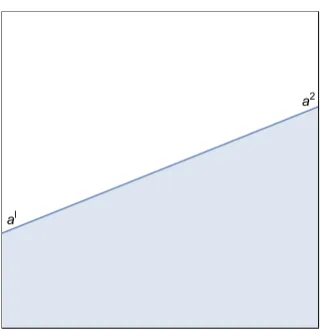
Example 2.2.1. Let D = [0,1]2_, _{Λ = [0}_,_1]2 _and _N _{= 2}_{. We specify points} _a _and

b on either side of the square D and join them with a straight line. We then let

A1(a, b) be the region ofD below this line and A2(a, b) =D\A1(a, b). Example sets

(29)

0.0 0.2 0.4 0.6 0.8 1.0 0.0 0.2 0.4 0.6 0.8 1.0

Figure 2.2: Possible setsAi corresponding to Example 2.2.1

Example 2.2.2. Let D = [0,1]2, Λ = [0,1]2 and N = 2. Choose a continuous

map H : Λ → L∞([0,1]) such that H(a, b)(0) = a and H(a, b)(1) = b for all

(a, b)_∈Λ. LetA1(a, b)be the region ofDbeneath the graph of the curveH(a, b) and

let A2(a, b) =D\A1(a, b). This setup includes the previous example: H(a, b)(x) = a+ (b−a)x defines the appropriate straight lines.

The continuity ofA1 and A2 can be seen by noting that

|A1(a1, b1)∆A1(a2, b2)|=|A2(a1, b1)∆A2(a2, b2)|

≤

Z 1

0 |

H(a1, b1)(x)−H(a2, b2)(x)|dx

≤ kH(a1, b1)−H(a2, b2)k∞

and using the continuity of H intoL∞_([0_,_1])_.

For example, one may takeH to be given by

H(a, b)(x) =a+ (b−a)x+xsin(6πx)/10

which can be seen to be continuous intoL∞_([0_,_1])_{. Example sets}_A

i(a, b)for various

parametersa, b, with this choice of H, are shown in Figure 2.3.

0.0 0.2 0.4 0.6 0.8 1.0 0.0 0.2 0.4 0.6 0.8 1.0

Figure 2.3: Possible setsAi, corresponding to Example 2.2.2

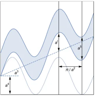
Example 2.2.3. We can generalize the previous example to allow the inclusion of

(30)

horizontal location of the fault. Given H : [0,1]2 _→ _L∞_([0_,_1]) _{as in the previous}

example, defineH˜ : Λ→L∞([0,1]) by

˜

H(a, b, c)(x) =

 



H(a, b)(x) x_∈[0, p]

c+H(a, b)(x) x∈(p,1]

so that the parameter c determines the (signed) magnitude of the fault. Defining the sets A1(a, b, c) and A2(a, b, c) as the regions of D beneath and above the curve

˜

H(a, b, c)respectively, the continuity can be seen in a similar manner to the previous example. Example sets Ai(a, b, c) for various parameters a, b, c are shown in Figure

2.4.

0.0 0.2 0.4 0.6 0.8 1.0 0.0 0.2 0.4 0.6 0.8 1.0

Figure 2.4: Possible setsAi, corresponding to Example 2.2.3 in the casep= 1/2.

Example 2.2.4. Again working with D= [0,1]2_{, but with a much larger parameter}

space, one could also select points at specific x-coordinates and linearly interpolate between them. FixK, N ∈Nand set Λ = ΞKN−1⊆[0,1](N−1)×K, where ΞN−1 is the

simplex

ΞN−1 ={(y1, . . . , yN−1)∈[0,1]N−1|0≤y1 ≤. . .≤yN−1 ≤1}.

Then given a _∈ Λ, define the functions fi(a), i = 1, . . . , N −1, to be the linear

interpolation of the points _Kj−₋1₁, aij

K

j=1. The sets Ai(a), i = 1, . . . , N −1, are

then defined to be the regions between the graphs of the functionsfi(a) and fi−1(a),

and AN(a) =D\ ∪Ni=1−1Ai(a). Note that the sets (Ai(a, b))Ni=1 are disjoint for fixed a, b_∈Λ by the choice of Λ. Example sets Ai(a, b) for various parameters a, b, with

this choice of H, are shown in Figure 2.5.

In order to see the continuity of these maps, we first partition the domain into strips

Dj,

Dj =

(x, y)_∈D

j₋1

K₋1 ≤x≤

j K₋1

(31)

so that we have

Ai(a) = K−1

[

j=1

Ai(a)∩Dj.

It follows from properties of the symmetric difference that

|Ai(a)∆Ai(b)| ≤ K−1

X

j=1

|(Ai(a)∩Dj)∆(Ai(b)∩Dj)|.

It hence suffices to show that the maps Ai(·)∩Dj are continuous for all i, j. This

follows from the same argument as in Example 2.2.2, for sufficiently small_|a₋b_|.

0.0 0.2 0.4 0.6 0.8 1.0 0.0

0.2 0.4 0.6 0.8 1.0

0.0 0.2 0.4 0.6 0.8 1.0 0.0

0.2 0.4 0.6 0.8 1.0

0.0 0.2 0.4 0.6 0.8 1.0 0.0

0.2 0.4 0.6 0.8 1.0

0.0 0.2 0.4 0.6 0.8 1.0 0.0

0.2 0.4 0.6 0.8 1.0

Figure 2.5: Possible sets Ai, corresponding to Example 2.2.4 in the case K = 11,

N = 6

2.2.2 The Darcy Model for Groundwater Flow

We consider the Darcy model for groundwater flow on a domainD⊆Rd,d= 1,2,3.

Letκ = (κij) denote the permeability tensor of the medium, p the pressure of the

water, and assume the viscosity of the water is constant. Darcy’s law [37] tells us that the velocity is proportional to the gradient of the pressure:

v=₋κ_∇p.

Additionally, a local form of mass conservation tells us that

(32)

wheref is a recharge term. Combining these two equations, and imposing Dirichlet boundary conditions for simplicity, results in the PDE

 



−∇ ·(κ_∇p) =f inD p=g on ∂D.

This is the PDE we will consider in the forward model, and it gives rise to a solution mapκ_7→p.

For simplicity we will work in the case whereκ is an isotropic (scalar) permeability, bounded above and below by positive constants, and so it can be represented as the image of some bounded function under a positive continuously differentiable map

σ:R→R+.

LetV =H1(D), the Sobolev space of square integrable once weakly differentiable functions on D [55]. Then given f _∈ H−1₍_D_), _g _∈ _H1/2₍_∂D_), _u _∈ _X _and _a _∈ _Λ,

definepu,a∈V to be the solution of the weak form of the PDE

 



−∇ ·(σ(ua₎_∇_p

u,a) =f inD

pu,a =g on ∂D.

(2.2.2)

We are first interested in the regularity of the map _R : X _×Λ _→ V given by

R(u, a) =pu,a. We first recall what it means forpu,ato be a solution of (2.2.2). Since

g _∈H1/2₍_∂D_{), by the trace theorem [55] there exists} _G _∈_V _{such that tr(}_G_{) =} _g_.

The solution pu,a of (2.2.2) is then given by pu,a = qu,a+G, where qu,a ∈ H01(D)

solves the PDE

 



−∇ · σ(ua₎_∇_q u,a

=f +∇ · σ(ua₎_∇_G

inD

qu,a = 0 on∂D.

(2.2.3)

The following lemma tells us that the map_Ris well defined and has certain regularity properties. Its proof is given in the appendix.

Lemma 2.2.5. The mapR:X×Λ→V is well-defined and satisfies:

(i) for each (u, a)_∈X_×Λ,

(33)

where κmin(u, a) is given by

κmin(u, a) = essinf

x∈D σ(u

a₍_x₎₎_>₀

and kfkV∗ denotes the dual norm of f as defined in the Appendix;

(ii) for each a∈Λ, _R(·, a) :X→ V is locally Lipschitz continuous, i.e. for every

r >0 there exists L(r) > 0 such that, for all u, v _∈ X with _ku_kX,kvkX < r

and all a∈Λ, we have

kR(u, a)_{− R}(v, a)_kV ≤L(r)ku−vkX;

(iii) for each u_∈X, _R(u,_·) : Λ_→V is continuous.

We now choose a continuous linear observation operator `:V _→RJ. For example,

writing`= (`1, . . . , `J), we could take

`i(p) =

Z

D

1 (2πε)d/2e

−|xi−y|2/2ε_p₍_y_{) d}_x, _i_{= 1}_{, . . . , J} _(2.2.4)

for some ε >0, so that `i approximates a point observation at the point xi ∈ D.

Our forward operator_G:X_×Λ_→RJ is then defined by G =`◦ R, so that it can

be written as the composition

(u, a)_7→ua_7→κ=σ(ua)_7→p_7→`(p)

From the above regularity of_Rwe can deduce the following regularity properties of our forward operatorG:

Proposition 2.2.6. Define the map _G:X_×Λ_→RJ as above. Then G satisfies

1. For each r >0 andu, v_∈X with _ku_kX,kvkX < r, there existsC(r)>0 such

that for all a∈Λ,

|G(u, a)_{− G}(v, a)_{| ≤}C(r)_ku₋v_kX.

2. For each u_∈X, the map _G(u,_·) : Λ_→RJ is continuous.

(34)

2. This follows from the continuity of` and Lemma 2.2.5(iii).

2.2.3 The Complete Electrode Model for EIT

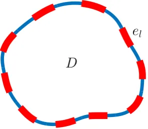
Electrical Impedance Tomography (EIT) is an imaging technique that aims to make inference about the internal conductivity of a body from surface voltage measure-ments. Electrodes are attached to the surface of the body, current is injected, and the resulting voltages on the electrodes are measured. Applications include both medical imaging, where the aim is to non-invasively detect internal abnormalities within a human patient, and subsurface imaging, where material properties of the subsurface are differentiated via their conductivities. Early references include [66] in the context of medical imaging and [90] in the context of subsurface imaging. The complete electrode model (CEM) is proposed for the forward model in [128], and shown to agree with experimental data up to measurement precision. In its strong form, the PDE reads

                        

−∇ ·(κ(x)∇v(x)) = 0 x∈D Z

el

κ∂v

∂ndS =Il l= 1, . . . , L κ(x)∂v

∂n(x) = 0 x∈∂D\ SL

l=1el

v(x) +zlκ(x)

∂v

∂n(x) =Vl x∈el, l = 1, . . . , L.

(2.2.5)

The domain D represents the body, and (el)L_l₌₁ ⊆ ∂D the electrodes attached to

its surface with corresponding contact impedances (zl)Ll=1. A current Il is injected

into each electrode el, and a voltage measurement Vl made. Here κ represents

the conductivity of the body, and v the potential within it. Note that the solution comprises both a functionv_∈H1₍_D_{) and a vector (}_V

l)Ll=1 ∈RLof boundary voltage

measurements.

A corresponding weak form exists, and is shown to have a unique solution (up to constants) given appropriate conditions on κ, (zl)Ll=1 and (Il)Ll=1 – see [128] for

details. Moreover, under some additional assumptions, the mapping κ_7→(Vl)Ll=1 is

(35)

D

[image:35.595.249.397.129.258.2]

e

l

Figure 2.6: An example domain D, with attached electrodes (el)Ll=1, for the EIT

problem.

We can apply different current stimulation patterns to the electrodes, that is, dif-ferent values of (Il)L_l₌₁ in (2.2.5), to yield additional information. Assume that

we haveM different (linearly independent) current stimulation patterns (I(m)₎M m=1.

This yieldsM different mappingsκ_7→(V_l(m))L

l=1 each with the regularity above, or

equivalently a mappingκ7→V whereV ∈RJ withJ =LM.

Analogously to the Darcy model case, we will consider isotropic conductivities of the formκ =σ(ua_{), where} _σ _:

R→ R+ is positive and continuously differentiable.

Our forward operator_G :X_×Λ_→RJ, is then given by the composition

(u, a)7→ua7→κ=σ(ua)7→ (v(1), V(1)), . . . ,(v(M), V(M))

7→(V(1), . . . , V(M)).

We show in the appendix that the map defined in this way has the same regularity as the map corresponding to the Darcy model.

Proposition 2.2.7. Define the map _G:X×Λ→RJ as above. Then G satisfies

1. For each r >0 andu, v_∈X with _ku_kX,kvkX < r, there existsC(r)>0 such

that for all a_∈Λ,

|G(u, a)− G(v, a)| ≤C(r)ku−vkX.

(36)

2.3 Onsager-Machlup Functionals and Prior Modelling

In this section we recall the definition of an Onsager-Machlup functional for a mea-sure which is equivalent1 to a Gaussian measure. We then introduce the prior measures that we will consider, first on the function space X, then the geometric parameter space Λ, and finally the product spaceX_×Λ. We conclude the section by extending the definition of Onsager-Machlup functional so that it is appropriate for the measures we consider here, supported on fields and geometric parameters which are combined to make piecewise continuous functions.

2.3.1 Onsager-Machlup Functionals

The Onsager-Machlup functional of a measure is the negative logarithm of its Lebesgue density when such a density exists, and otherwise can be thought of analo-gously. We start by defining it precisely for measures defined via density with respect to a Gaussian, allowing for infinite dimensional spaces on which the Lebesgue mea-sure is not defined. Suppose thatµ is a measure equivalent to a Gaussian measure

µ0; the definition of such measures is found in the Appendix. Then the

Onsager-Machlup functional forµis defined as follows.

Definition 2.3.1 (Onsager-Machlup functional I). Let µ be a measure on a

Ba-nach space Z which is equivalent to µ0, where µ0 is a Gaussian measure on Z with

Cameron-Martin space E. Let Bδ₍_z₎ _{denote the ball of radius} _δ _{centred at} _z _∈_Z_.

A functional I :Z → Ris called the Onsager-Machlup functionalfor µif, for each

x, y_∈E,

lim

δ↓0

µ(Bδ₍_x₎₎

µ(Bδ₍_y₎₎ = exp (I(y)−I(x))

andI(x) =_∞ for x /_∈E.

Remarks 2.3.2. (i) The Onsager-Machlup functional is only defined up to

addi-tion of a constant.

(ii) If Z is finite dimensional and µ admits a positive Lebesgue density ρ, then

I(x) = ₋logρ(x) for all x _∈ Z. In light of the previous remark, this is true even ifρ is not normalized.

1_{Two measures} _{ν, µ} _{on a measurable space (}_M,_M_{) are equivalent if} _ν₍_A_{) = 0 if and only if}

(37)

(iii) LetZ =Rnbe finite dimensional, and letµ0 =N(0,Σ)be a Gaussian measure

on Z. Let Γ ∈ Rm×m be a positive-definite matrix, A ∈ Rm×n and y ∈ Rm.

Defineµ by

dµ

dµ0

(x)∝exp

−1

2|Ax−y|

2 Γ

so that

dµ

dx(x)∝exp

−1

2|Ax−y|

2 Γ−

1 2|x|

2 Σ

.

Then by the previous remark, the Onsager-Machlup functional for µ is given by

I(x) = 1

2|Ax−y|

2 Γ+

1 2|x|

2 Σ

for allx∈Z, which is a Tikhonov regularized least squares functional.

(iv) The preceding example (iii) may be extended to an infinite dimensional setting.

Let Z be a separable Banach space, and let µ0 = N(0,C0) be a Gaussian

measure onZ with Cameron-Martin space(E,h·,·iE,k · kE). LetΓ∈Rm×m be

a positive-definite matrix,A:X_→Rm a bounded linear operator andy∈Rm.

Defineµ by

dµ

dµ0(x)∝exp

−1

2|Ax−y|

2 Γ

.

Then Theorem 3.2 in [38] tells us that the Onsager-Machlup functional for µ

is given by

I(x) = 1

2|Ax−y|

2 Γ+

1 2kxk

2

E.

(v) In this chapter, the posterior distribution will be a measure on the product

space Z = X ×Λ. The prior distribution will be an independent product of a Gaussian on X and a compactly supported measure on Λ. Due to the assumption of compact support, the prior will not be equivalent to a Gaussian

measure on Z and so the above definition doesn’t apply; we provide a suitable extension to the definition in subsection 2.3.4.

(38)

measures onX and Λ. We will combine these into a prior measure on the product space X ×Λ. We equip this space with any (complete) norm k(·,·)k such that if

k(u, a)_{k →}0, then _ku_kX →0 and |a| →0.

2.3.2 Priors for the Fields

We wish to put priors on the fields u1, . . . , uN ∈ C0(D). We use independent

Gaussian measuresui ∼ µi₀ := N(mi,Ci), where the means mi ∈C0(D), and each

covariance operator Ci : C0(D) → C0(D) is trace-class and positive definite. It

follows that the vector (u1, . . . , uN)∼µ10×. . .×µN0 =:µ0 is Gaussian onX:

µ0 =N m,

N

M

i=1

Ci

!

wherem= (m1, . . . , mN)∈X. If Ei denotes the Cameron-Martin space [39] of µi₀,

then that ofµ0 is given by

E=

N

M

i=1 Ei

with inner product given by the sum of those of its component spaces. The Onsager-Machlup functional ofµ0 is known to be given by

J(u) =

 

 1

2ku−mk2E u−m∈E

∞ u₋m /_∈E.

This can be seen, for example, as a consequence of Proposition 18.3 in [97].

Remark 2.3.3. We may assume that the different fields are correlated under the

prior, so long asµ0remains Gaussian onX– this does not affect any of the following

theory. Allowing correlations between the fields and the geometric parameters under the prior is a more technical issue however, and so we will assume that these are

independent.

Example 2.3.4. Define the negative Laplacian with Neumann boundary conditions

as follows:

A=₋∆, _D(A) =

u_∈H2(D)

du

dν = 0 on∂D, Z

D

u(x) dx= 0

(39)

ThenA is invertible. We can define_Ci=A−αi, where each αi> d/2. Then eachCi

is trace-class and positive definite, and samples from each µi

0 will be almost surely

continuous and so µ0 can be considered as a Gaussian measure on X. Moreover,

regularity of the samples will increase as αi increases, see [39] for details.

2.3.3 Priors for the Geometric Parameters

We also want to put a prior measure on the geometric parameters, i.e. we want to choose a probability measure on Λ. Since Λ⊆Rk the analysis is more

straight-forward than the infinite dimensional case. Let ν be a probability measure on Λ with compact support S ⊆Λ. We assume ν is absolutely continuous with respect to the Lebesgue measure and that its density ρ is continuous on S. Despite being defined on a finite dimensional space, the measureν is not necessarily equivalent to the Lebesgue measure on the whole ofRk and so the previous definition of

Onsager-Machlup functional does not apply. We hence must formulate a new definition for this case.

Sinceρ >0 on int(S), we can use the continuity ofρto calculate the limits of ratios of small ball probabilities forν on int(S). Leta1, a2 ∈int(S), then

lim

δ↓0

ν(Bδ₍_a

1)) ν(Bδ₍_a2₎₎ = lim_δ_↓₀

R

Bδ₍_a

1)ρ(a) da

R

Bδ₍_a

2)ρ(a) da

= lim

δ↓0 1

|Bδ₍_a

1)|

R

Bδ₍_a

1)ρ(a) da

1

|Bδ₍_a

2)|

R

Bδ₍_a

2)ρ(a) da

= ρ(a1)

ρ(a2)

= exp (logρ(a1)−logρ(a2)).

If eithera1 ora2 lie outside ofS the limit can be seen to be 0 or ∞respectively. It

hence makes sense to define the Onsager-Machlup functional forνon Λ\∂Sas

K(a) =

 



−logρ(a) a∈int(S)

∞ a /_∈S.

Fora_∈∂S, we define K(a) to be the limit ofK from the interior:

K(a) =− lim

b→a b∈int(S)

(40)

which is well defined due to the continuity ofρ on int(S). K is then continuous on the whole ofS.

Remark 2.3.5. If we were to define K on ∂S in the same way that we defined it

onΛ_\∂S, K would have a positive jump at the boundary related to the geometry of

S. This would mean thatK was not lower semi-continuous onS which would cause problems when seeking minimizers. The definition we have chosen is appropriate: if any minimizing sequence(an)n≥1 ⊆int(S) of K has an accumulation point on ∂S,

thenν has a mode at that point.

If we have no prior knowledge about the interfaces and Λ is compact, we could place a uniform prior on the whole of Λ. Otherwise we could either choose a prior with smaller support, or one that weights certain areas more than others.

2.3.4 Priors on X_×Λ

We assume that the priors on the fields and the geometric parameters are indepen-dent, so that we may take the product measure µ0 ×ν0 as our prior on X×Λ.

Note that ifF :X_×Λ_→L∞₍_D_{) denotes the construction map (}_{u, a}₎_7→_ua _defined

earlier by (2.2.1), then our prior permeability/conductivity distribution onL∞(D) is given by the pushforwardµ∗

0 =F#(µ0×ν0), where the pushforward is as defined

in the Appendix. This is much more cumbersome to deal with however, since for exampleL∞(D) is not separable. It is for this reason we incorporate the mappingF

into the forward map_G. Assuming now that the priorµ0×ν0 is as described above,

we can define the Onsager-Machlup functional for measuresµ on X_×Λ which are equivalent toµ0×ν0.

Definition 2.3.6 (Onsager-Machlup functional II). Let µ be a measure on X×Λ

equivalent to µ0 ×ν0, where µ0 and ν0 satisfy the assumptions detailed above. Let Bδ₍_{u, a}₎ _{denote the ball of radius} _δ _{centred at} ₍_{u, a}₎ _∈ _X _×_Λ_{. A functional} _I _:

X_×Λ_→R is called the Onsager-Machlup functional for µ if,

(i) for each (u, a),(v, b)_∈E_×int(S),

lim

δ↓0

µ(Bδ₍_{u, a}₎₎

(41)

(ii) for each (u, a)_∈E_×∂S,

I(u, a) = lim

b→a b∈int(S)

I(u, b);

(iii) I(u, a) =∞ for u /∈E or a /∈S.

2.4 Likelihood and Posterior Distribution

We return to the abstract setting mentioned in the introduction. LetX be a sep-arable Banach space, Λ_⊆ Rk and Y = RJ. Suppose we have a forward operator

G:X×Λ→Y. If (u, a) denotes the true input to our forward problem, we observe datay_∈Y given by

y=G(u, a) +η

where η _∼ Q0 := N(0,Γ), Γ ∈ RJ×J positive definite, is Gaussian noise on Y

independent of the prior.

It is clear that we havey_|(u, a)_∼Qu,a:=N(G(u, a),Γ). We can use this to formally

find the distribution of (u, a)|y. First note that

Qu,a(dy) = exp

−Φ(u, a;y) + 1 2|y|

2 Γ

Q0(dy)

where the potential (or negative log-likelihood) Φ :X_×Λ_×Y _→Ris given by

Φ(u, a;y) = 1

2|G(u, a)−y|

2

Γ. (2.4.1)

Hence under suitable regularity conditions, Bayes’ theorem tells us that the distri-butionµ of (u, a)_|y satisfies

µ(du,da)_∝exp ₋Φ(u, a;y)

µ0(du)ν0(da)

after absorbing the exp 1₂|y|2 Γ

term into the normalisation constant.

Analysis and computation for Bayesian inverse problems

warwick.ac.uk/lib-publications

A Thesis Submitted for the Degree of PhD at the University of Warwick

Permanent WRAP URL:

http://wrap.warwick.ac.uk/86136

Copyright and reuse:

This thesis is made available online and is protected by original copyright.

Please scroll down to view the document itself.

Please refer to the repository record for this item for information to help you to cite it.

Our policy information is available from the repository home page.

M A

O

D

C

S

Analysis and Computation for Bayesian

Inverse Problems

Matthew M. Dunlop

Thesis

Doctor of Philosophy

Mathematics Institute

The University of Warwick

Contents

Acknowledgments

Declarations

Abstract

Chapter 1

Introduction

1.1

Overview

1.2

Outline of the Thesis

Chapter 2

MAP Estimators for Piecewise

Continuous Inversion

2.1

Introduction

2.2

The Forward Problem

D

e

2.3

Onsager-Machlup Functionals and Prior Modelling

2.4

Likelihood and Posterior Distribution