Computational studies of paddlewheel complexes in isolation and incorporated into metal organic frameworks

(1)

warwick.ac.uk/lib-publications

A Thesis Submitted for the Degree of PhD at the University of Warwick

Permanent WRAP URL:

http://wrap.warwick.ac.uk/95507

Copyright and reuse:

This thesis is made available online and is protected by original copyright. Please scroll down to view the document itself.

Please refer to the repository record for this item for information to help you to cite it. Our policy information is available from the repository home page.

(2)

Computational Studies of Paddlewheel Complexes in

Isolation and Incorporated into Metal Organic

Frameworks

By

Khalid Ahmad Alzahrani

A thesis submitted in partial fulfilment of the requirements for the

degree of Doctor of Philosophy in Chemistry

Department of Chemistry,

University of Warwick,

CV4 7AL

(3)

Tables and Illustrations

Figure 1.1; Potential applications of metal organic frameworks (MOFs)...15

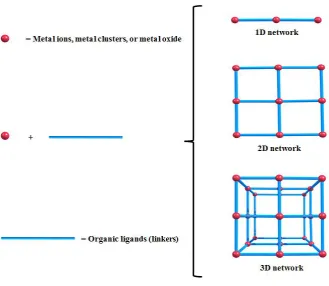
Figure 1.2; Schematic representation of one-, two-, or three-dimensional structures of MOFs built from metal units and organic ligands (linkers)...16

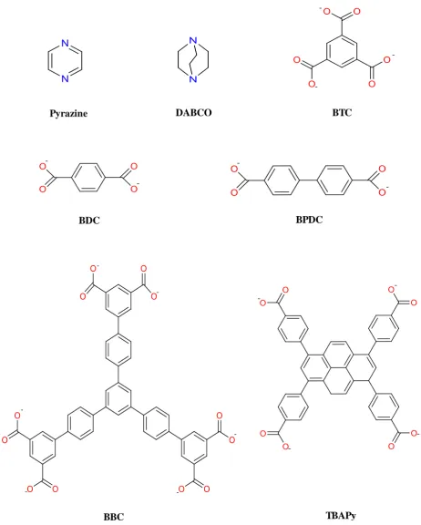
Figure 1.3; Some organic linkers used in producing the most useful MOF systems. Pyrazine and DABCO are usually used as axial linkers………..….17

Figure 1.4; Schematic view of some MOFs built from metals unit and organic linkers (ligands). MOF-5 built from Zn4O nodes with 1,4-benzodicarboxylic acid linkers, HKUST-1 built from copper nodes with 1,3,5-benzenetricarboxylic acid between them, and MIL-53 built from scandium and oxygen (ScO6_{) nodes with} 1,4-benzodicarboxylic acid linkers between the nodes. These structures are adapted from ChemTube3D home website, University of Liverpool...18

Figure 1.5; Schematic representation of four-bladed paddlewheel complex...19

Figure 1.6; Pore framework structures for [Zn2(bdc)2(dabco)]n derived from published CIF files. Hydrogens and encapsulated solvent removed. dabco and carboxylate disorder as per CIF file...19

Table 2.1; Scaling of different QM methods with respect to the number of electrons n...37

Figure 2.1; The model of molecular mechanics...44

Figure 2.2; Angles bending of central atom for different common geometries...49

Figure 2.3; Experimental hydration enthalpies values from Ca2+_(d0_{) through to Zn}2+ (d10_{). The open circles expressed the values once the effects of LFSE are removed..51}

(7)

2

Figure 2.6; Comparison between CFT barycentre (left) and AOM barycentre (right) in case of a π-donor ligand where eπ is positive...53

Figure 2.7; Schematic representation of ligand and coordination regions and force field terms which represent them...54

Figure 3.1; Pore framework structures for [Zn2(bdc)2(dabco)]n derived from published CIF files.12_{Hydrogens and encapsulated solvent removed. dabco and carboxylate} disorder as per CIF file...59

Figure 3.2; Local detail of carboxylate coordination in WUHHEN. Bond lengths (Å) shown in dark red. The upper Zn-O contact is anomalously short, the carboxylate C-O bonds too asymmetric and one hydrogen is missing off the highlighted carbon (grey sphere)...64

Figure 3.3; Packing detail for TUFLOW showing intermolecular H-bond contacts (dotted magenta oval) responsible for the long Zn-O distance. (The extra connecting molecules top right and bottom left are omitted for clarity as are all the H atoms bar those involved in the H-bond.)……….65

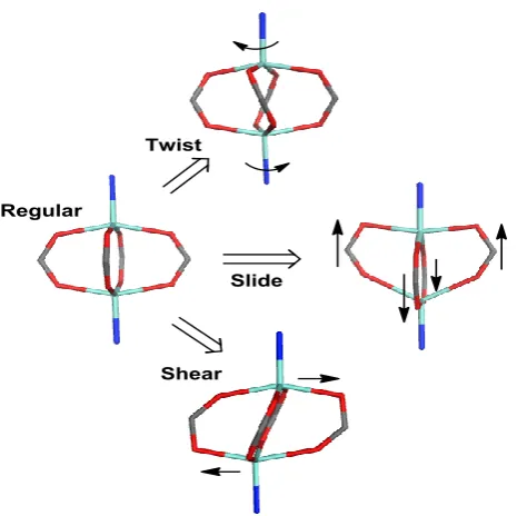
Figure 3.4; Schematic idealizations of possible distortions of a regular zinc paddlewheel structure...66

Figure 3.5; A selection of entries from the CSD used to validate the DFT protocol..67

Figure 3.6; Overlays of X-ray (yellow) and DFT-optimized (blue) structures for selected ZPW systems. Hydrogen omitted for clarity...68

Table 3.1; Comparison of experimental and calculated bond lengths (Å) for the complexes shown in Figure 3.5. The O(CBX) entry is the averaged Zn-O(carboxylate) distance. Zn-L refers to the bond to the capping group...69

Figure 3.7; Schematic representation of the ZnPR.nL systems used for initial training...71

(8)

3

Figure 3.8; Comparison of optimized DFT and MM (in parentheses) structural parameters for ZnPH.nL, (n = 0, 1, 2; L = NH3, py). Only unique Zn-L and L-Zn-L data shown. Distances in Å and angles in degrees. Hydrogens omitted for clarity. Depicted structures are from DFT-optimized coordinates...74

Table 3.3; Calculated Zn-O bond lengths (Å), activation energies (kcal mol-1_{) and} transition-state frequencies (cm -1_{) for ZnPR transition state systems, R = H, CH}

3 and CF3...75 Table 3.4; Performance of ZPW-FF for molecules shown in Figure 3.9. Column 1 CSD refcodes. Column 2, root mean square deviation for Zn-L bond lengths. Column 3, root mean square deviation for heavy atom (i.e. non-hydrogen) overlay. Column 4, difference between experimental and computed Zn-Zn distance (a negative value implies a shorter computed value). All numerical data in Å...76

Figure 3.9; Structural diagrams of ligands for the ZPW systems listed by CSD refcode in Table 3.4. Only unique combinations displayed. (NEHZUV and NEHHUV01 are the same compound while INIBAJ and QETGAY have the same ligand set)...77

Figure 3.10; Starting pore model for MM optimizations derived from X-ray diffraction study. Positions of experimental water molecules are shown but waters are not included in the MM calculations...79

Figure 3.11; Development of the ‘breathing’ for [Zn(bdc)2(dabco)]n.solvate. Left column displays the single pore starting model for MM optimization. Central column shows the ZPW-FF optimized structure of the single pore model. The right column shows the ZPW-FF optimized structure of the central pore of the nine-pore 3x3 grid...80

(9)

4

Figure 3.13; Plot of distances from a corner zinc centre to the N atom of the five DMF molecules in the central pore of the 3x3 grid during the simulated annealing MD run showing how one of the DMF molecules (N1) is spontaneously ejected from the central pore...84

Figure 4.1; Pore framework structures for [Zn2(bdc)2(dabco)]n derived from published CIF files.16_{Hydrogens and encapsulated solvent removed. dabco and carboxylate} disorder as per CIF file...93

Figure 4.2; Schematic illustration of decomposition pathway of Zn(bdc)(dabco)0. 5 reacting with water molecules...95

Figure 4.3; Horizontal viewing of the two layers stacking model in the crystals of MOF-2 showing H-bonding interactions (green dot line) between them...95

Figure 4.4; Local detail of carboxylate coordination in WUHHEN. Right structure shows the X-ray anomalously data and the left one shows the DFT-optimized structure. Bond length (Å) shown in dark red. One hydrogen is missing off the highligh ted carbon (gray sphere)...99

Figure 4.5; Optimized DFT structure of Zn2PCH3.2H2O system showing TBP geometry for zinc centres (Zn blue, O red, C gray and H white)...100

Figure 4.6; Schematic representation of the ZnPR.nL systems used for initial training...101

Table 4.1; The partial atomic charges for MMFF94 implementation of ZPW-FF. Standard MMFF94 charges in parentheses...102

Figure 4.7; The possible rotations of the apical water ligand those identify the ZPW motif geometries. These models are obtained by MM optimization which are clearly revealed both geometries based on the rotations of water...104

Figure 4.8; Overlays of DFT (blue) and MM-optimised (Red) structures for the available ZPW systems. Hydrogens omitted for clarity………….………105

(10)

5

Figure 4.9; ZPW-FF simulated annealing starting from the energy-optimized, 1 pore model showing that of the guest molecules (benzene blue, left and DMF dark green, right) ejected the pore from the water top surface side. The DMF model has shown H-bonding between water molecule and the DMF (highlighted by dotted green line)..106

Figure 4.10; The new charge scheme for DMF guest molecules inside MOF-2 cavities...108

Figure 4.11; The MM-optimized neutral two-dimensional layered framework of MOF-2 without DMF quest molecules. The top represents the optimized structure along the vertical direction, while the down along the horizontal direction….……..109

Figure 4.12; MM calculations of 3D layer-by-layer model in the crystal of MOF-2. The top model is the MM-optimized structure, the bottom is MD annealing of the top. The DMF guest molecules are represented with space-filling spheres. The yellow spheres for the DMF molecules held in voids by vdW interaction with bdc linker, dark blue spheres for ejected DMF molecules, and the green spheres for the DMF molecules held by inter water ligand. Almost Each voids held 2 DMF guest molecules…...….111

Figure 5.1; Unit cell of [Zn(bdc)2(dabco)]n. Left: as-synthesised material with four dimethylformamides and a water molecule; centre: after evacuation; right: after uptake of four benzene molecules. (Adsorbed species and H atoms omitted for clarity.)...118

Figure 5.2; Schematic representation of four-bladed paddlewheel complex...118

Figure 5.3; Centre: selected calculated geometrical data for [Cu2(formate)4(NH3)2]. Normal text for elongated dx2–y2/dx2–y2 state (T0) structure; italics for mixed dx2–y2/dz2 state (TM) structure. Spin density plots to left and right...122

Figure 5.4; Schematic partial valence molecular orbital (MO) energy level diagram for copper paddlewheel systems as a function of increasing the axial ligand field. For the MOs, S refers to a symmetric (in-phase) combination of d orbitals, A to an asymmetric combination, Ax = dz2 and Eq = dx2–y2...123

(11)

6

Figure 5.5; Optimised geometries for [Cu2(acetate)4(Me2NHC)2]. Top: complete structures; Middle and bottom: local geometrical detail around the metal centres. Numbers with two decimal places are distances in Å; those to one decimal place are angles in °...126

Figure 5.6; Spin density (left) and plots of the molecular orbital housing the two unpaired electrons for the symmetric TBP structure shown in Figure 5.5, left...127

Figure 5.7; Schematic diagram of the sense of Jahn–Teller elongation (highlighted in pink) for CPW–NHC systems...127

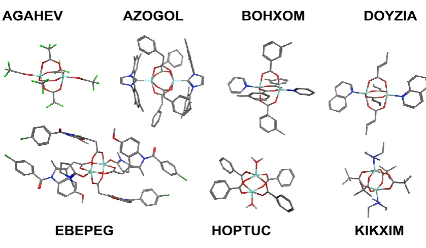
Figure 5.8; Illustrative metal–NHC complexes. AZOGOL is a zinc–NHC paddlewheel [Zn2(OC2CH2Ph)4(N-MesitylNHC)2] while QAXKAC is Cu(II)–{bis- (2,5-iPrPh)NHC}(acetate)2. For the Zn complex, yellow corresponds to the X-ray structure, blue to the DFT optimisation. The CPW is also the computed geometry (BP86/SVP/D3/COSMO)...129

Figure 6.1; Schematic representation of CPWs building units within MOFs...134

Figure 6.2; Schematic representation of the CuPR.nL systems used for initial training data...137

Figure 6.3; DFT optimized structures of some CPWs models. It is clear that the CPWs units are usually elongated structure. However, (H) forms compressed structure because the presence of strong axial ligand filed (NHC) in combination with weak carboxylate specie (trifluoroacetate). The atoms are coloured for clarity (Cu = dark blue, O = red, N = pink, and C = yellow, F = white-yellow, and H = blue)………...139

Figure 6.4; Schematic partial valence molecular orbital (MO) energy level diagram for copper paddlewheel systems as a function of increasing the axial ligand field. For the MOs, S refers to a symmetric (in-phase) combination of d orbitals, A to an asymmetric combination, Ax = dz2 and Eq = dx2–y2...140

(12)

7

Figure 6.6; Introduction of AOM parameters of local M-L bonding showing the differences between σ and π interactions……….142

(13)

8

Acknowledgements

Firstly I would like to acknowledge the support of the King Abdulaziz University and the Ministry of Education, Kingdom of Saudi Arabia, for the provision of a PhD scholarship as without their support this PhD would not have happened.

I would like to acknowledge the University of Warwick for providing me everything needed for writing up this thesis. Many thanks to the Royal Society of Chemistry for allowing me to access the Cambridge Structural Database.

I would like to acknowledge the efforts of my supervisor Prof. Robert Deeth who has guided me through the last four years, offered invaluable support and more recently has assisted in proof reading half of this thesis. I would also like to thank my second supervisor Dr. Scott Habershon for his great support and advice through the last two years (After RD took early retirement in 2015), and for his assistance in proof reading the second half of this thesis. My thanks to Ben Houghton for helping organise and focus me at the beginning, and to Scott’s and Alessandro’s group members for their support in the last two years. Many thanks to all my Saudi friends in Coventry for the enjoyable gathering meetings during weekends and holydays.

(14)

9

Declaration

This thesis is submitted to the University of Warwick in support of my application for the degree of Doctor of Philosophy. It has been composed by myself and has not been submitted in any previous application for any degree.

The work presented was carried out by the author, including data generated and data analysis except in the cases outlined below:

 The SVL coding files in Chapter 3 and Chapter 4 were written by Robert J.

Deeth (PhD supervisor).

 The DFT calculations in Chapter 5 using ADF software were carried out by

Robert J. Deeth.

Parts of this thesis have been published by the author:

 K. A. H. Alzahrani and R. J. Deeth, J. Mol. Model., 2016, 22, 80.

 K. A. H. Alzahrani and R. J. Deeth, Dalton Trans, 2016, 45, 11944-11948.

(15)

10

Abstract

The aim of the work presented in this thesis is to develop computational approaches to the modelling of zinc and copper paddlewheel complexes both in isolation and when

incorporated into metal organic frameworks (MOFs). We considered both ‘ab initio’

and empirical force field methods based mainly on DFT and ligand field molecular mechanics (LFMM) respectively.

(16)

11

In the second part of this thesis, our density functional theory calculations on four-bladed copper paddlewheel (CPW) systems [Cu2(O2CR)4L2] reveal a change in ground state with increasing Cu–L bond strength. For L = N-heterocyclic carbene (NHC), the Jahn–Teller axis switches from parallel to orthogonal to the Cu–Cu vector and the copper coordination geometry becomes highly flexible. While the calculated dimer/monomer equilibrium for isolated complexes slightly favours monomers, the preformed paddlewheel units embedded in many metal organic frameworks are potential targets for developing novel materials. Therefore, the preliminary LFMM parameters for constructing a generic CPW-FF are reported. However, a definitive version of the CPW-FF remains a task for the future.

(17)

12

Abbreviations

MOF – Metal Organic Framework

ZPW – Zinc Paddlewheel

CPW – Copper Paddlewheel

ZPW-FF – Zinc Paddlewheel Force Field

CPW-FF – Copper Paddlewheel Force Field

CSD – Cambridge Structure Database

DFT – Density Functional Theory

HF – Hartree Fock

ADF – Amsterdam Density Functional

QM - Quantum Mechanics

MOE – The Molecular Operating Environment

DommiMOE – d-Orbital Molecular Mechanics in MOE MM - Molecular Mechanics

MD – Molecular Dynamic

LFMM – Ligand Field Molecular Mechanics

LFSE - Ligand Field Stabilization Energy

LFT – Ligand Field Theory AOM – Angular Overlap Model

FF – Force Field

(18)

13

Chapter 1: Introduction to Metal Organic Frameworks

1.1 Motivation

“What would happen if we could arrange the atoms one by one the way we want

them?” This is one of the most famous questions in material science, which was asked,

in 1959, by Richard P. Feynman. Since then, chemists have tried to answer the question by involving themselves intensively in studying the structures and interactions of molecules and atoms in gases, liquids and solids. From our perspective, a partial answer of Feynman’s question is to identify which effects are important for

the controlled arrangement or rearrangement of molecules or atoms.

This work deals generally with crystalline porous materials where the atoms are arranged to generate ordered pores within structures. In addition, changing the pore size and/or shape by modifying the structure itself or the adsorbed molecules are mainly considered in this work. Therefore, applying Feynman’s question to these kind of compounds, would lead chemists to define the cavities on a molecular level.

(19)

14

‘‘Soft porous crystals are defined as porous solids that possess both a highly ordered

network and structural transformability. They are bistable or multistable crystalline

materials with long range structural ordering, a reversible transformability between

states, and permanent porosity. The term porosity means that at least one crystal phase

possesses space that can be occupied by guest molecules, so that the framework

exhibits reproducible guest adsorption’’ (quoted from S. Horike et al.) 1

(20)

15

1.2 Metal organic frameworks (MOFs)

Metal-organic frameworks (MOFs), also known as coordination networks or coordination polymers in the literature, are now considered as one of the most promising classes of porous materials.2-6_{Over the past fifty years, research into such} materials has resulted in many applications which have affected our lives and industrial processes (Figure 1.1).7-13_{MOFs are crystalline materials consisting of central metal} ions, metal clusters, or metal oxide clusters and organic ligands acting as linkers to

form one-, two-, or three-dimensional structures (Figure 1.2).14-16

(21)

16

Figure 1.2; Schematic representation of one-, two-, or three-dimensional structures of MOFs built from metal units and organic ligands (linkers).

[image:21.595.151.481.82.368.2]

(22)

17

Figure 1.3; Some organic linkers used in producing the most useful MOF systems. Pyrazine and DABCO are usually used as axial linkers.

Pyrazine DABCO

BDC

BTC

BPDC

[image:22.595.80.543.84.661.2]

(23)

18

Since the pioneering work of Robson and co-workers 20_{thousands of scientific} articles, which feature the term ‘metal-organic framework’, have been published.

Yaghi, Fujita, Zaworotko, Kitagawa, Moore/Lee, and Ferey research groups have contributed to produce a number of MOFs systems (such as MOF-5, HKUST-1 21_, MIL-53 22_{etc.) which are built from different metals connected by a variety of organic} linkers (Figure 1.4)

Figure 1.4; Schematic view of some MOFs built from metals unit and organic linkers (ligands). MOF-5 built from Zn4O nodes with 1,4-benzodicarboxylic acid linkers, HKUST-1 built from copper nodes with HKUST-1,3,5-benzenetricarboxylic acid between them, and MIL-53 built from scandium and oxygen (ScO6) nodes with 1,4-benzodicarboxylic acid linkers

between the nodes. These structures are adapted from ChemTube3D home website, University of Liverpool.

Theoretically, the plentiful sources of organic linkers and metals ions lead to design of a wide variety of MOFs. However, in this thesis, the flexible MOFs containing a paddle-wheel secondary building units (SBUs), where the paddle-wheel motif is a transition metal (TM) dimer bridged by four carboxylate units is emphasized (Figure 1.5). While many MOFs have relatively rigid frameworks which therefore define a fixed pore size, other MOFs display a degree of flexibility or ‘breathing’ (Figure

(24)

19

1.6).23, 24_{The pore size and/or shape changes as a function of adsorbate offering} exciting possibilities for using these materials particularly in separations25-28_and sensing29, 30_{. As mentioned previously, some flexible MOFs systems contain a paddle} -wheel SBU. The paddle--wheel motif is a TM dimer bridged by three or four carboxylate units. In combination with linear linkers, the latter generates planar [M2L2]n grids which can be interconnected by ditopic pillars like 1,4-diazabicyclo(2.2.2)octane (dabco) or pyrazine to generate a 3-D framework.

Figure 1.5; Schematic representation of four-bladed paddlewheel complex.

[image:24.595.223.412.302.457.2]

(25)

20

1.3 Current and Potential applications of MOFs

Nanoporous materials, such as zeolites, carbon nanotubes, activated carbon, and MOFs have been used widely in several energy-related applications.7, 31_{However, due} to their crystalline nature, the potential applications of MOFs are much greater than other Nanoporous materials. Additionally, the ability of introducing different functional groups through their hybrid framework makes MOFs a promising candidates for a variety of applications. All of these features motivate scientists to

obtain unique porous materials with various functionality and selectively as well. In this introduction, therefore, the potential applications of MOFs have been classified into five broad groups which are presented below briefly. Although this thesis concentrates on modelling flexible MOFs systems, introducing some potential applications of MOFs systems, whether rigid or flexible, are crucial here to provide the readers a general information regarding the MOF systems and their applications.

1.3.1 Gas Storage and Delivery

(26)

21

hydrogen-fuelled automobiles. The development of a safe and viable approach for the storage of H2 would likely accelerate the wide spread commercialization of this application.34_{Beside the storage of H}

2 other molecules like carbon dioxide and methane which would be used within MOFs as a greenhouse gas and energy carrier applications respectively.35_{MOFs have also an abilities to store both small and large} molecule and release them in a controlled manner.36, 37_{This feature have been used} widely in pharmaceutical applications especially for drug delivery.38_Therefore, understanding the interactions between MOFs and guest molecules is highly essential in this area.

1.3.2 Gas Adsorption and Separation

The high porosity (the largest pore = 98 Å ) 39_{and surface areas (ranging from 1000} to 10,000 m2_/g)7_{properties of MOFs have nominated this type of materials to be an} excellent candidate for gas adsorption and separation applications. Compared to other inorganic porous materials, the pores in MOFs can be affected by systematically introducing functional groups into the framework. Thus, gas adsorption and separation characterisations of MOFs can be tuned, not only by changing the pore size and shape, but also by the specific tailoring of the interaction between guest molecules and frameworks. This property leads researchers to use MOFs for separation of liquid and gas mixtures.25-28

(27)

22

MOFs have widely play an important role in capturing the greenhouse gases (e.g. carbon dioxide, CO2) from industrial emissions, which contribute to global warming. 40-42_{In regard to the latter, some studies have shown the possibility of achieving}

kinetic-based separations using MOFs.43_{Therefore, understanding the interaction} between MOFs and guest molecule with respect to the mobility and the ordering of the guest species into the pores is very important.

1.3.3 Catalysis

(28)

23

All of these properties associated with MOF systems will attract more researchers to investigate the MOF-based catalysis applications in the near future. However, a better understanding of the reaction mechanism at the active centre is basically required. Moreover, studying the mobility and the ordering of all reactants within the pores are also needed to enhance systematically the performance of MOF-based catalysis.

1.3.4 Luminescent MOFs and Sensing

The presence of metals ions and organic linkers, with various functional groups, within MOFs have nominated these materials to be promising candidates as sources of emissive phenomena. It is known that luminescent materials have been widely used in making sensing, lighting, display, and optoelectronic devices. Nevertheless, nowadays, developing a suitable luminescent MOFs for practical applications is substantially interesting.31_{Moreover, producing MOFs-based sensing systems is} interesting at the moment.29, 30

(29)

24

detect some molecules, such as water and alcohols, which their adsorption does not required a large structural transformation.

1.3.5 Magnetic MOFs

In recent years, MOFs materials have been used in many applications based on their magnetics properties. The design possibilities that allow embedding paramagnetic metal ions such as Cu+2_{, or using open-shell organic linkers within MOFs would result}

in magnetic properties and strong magnetic interactions between the centres of spin.5 2 Moreover, the ligand diversity and topology design possibilities incorporated within MOFs can maximize and control the magnetic interactions between linker and/or metal sites to enhance system’s cooperativity. This type of materials are known as magnetic

framework composites (MFCs) which are recently used in many technological field such as catalysis, storage, drug delivery, imaging and sensing.53

1.4 Design and Characterization of MOFs

(30)

25

as gas storage, gas separation, gas adsorption, and catalysis, can be characterized. Despite that this approach is widely used, it is nevertheless time consuming and expensive especially for characterization.54-56

The second approach is to use computational modelling where the topologies of MOFs can be predicted and formed theoretically from various metal and organic linkers. This approach involves usually constructing large libraries of potential MOFs materials.57, 58_{The enumeration of MOF topologies would be followed by screening for targeted} properties such as higher pore sizes, presence of open metal sites, and stability and higher selectivity for certain gas molecules. The predicted MOFs with desired properties can be then synthesised and characterized experimentally.59_{For example,} Farah et al,8_{have initially used molecular simulations tools to design and characterize} a MOF system named NU-100 with a particularly high surface area which enables storage of hydrogen and carbon dioxide. Subsequently, NU-100 was synthesized and characterized experimentally yielded a material being in excellent agreement with calculated structure.

(31)

26

1.5 Computational Studies of MOFs

Exploring the properties of thousands of MOFs reported in the literature using available experimental techniques is very expensive and time consuming. Furthermore, some detailed information such as the microscopic properties of MOFs are very difficult to be studied using only experimental methods. Therefore, molecular modelling methods have provided a valuable complement to experimental studies giving researchers a deeper and more thorough understating of these materials at the

molecular level, including mechanisms of host-guest interactions involved.60-62_In addition, molecular modelling has been used significantly by chemists and engineering for large-scale screening of hypothetical and existing materials, including MOFs.58 Thus, during the past decade, significant computational approaches studies have been done for investigating the performance and properties of MOFs.14-16

(32)

27

specific adsorption and transport applications of MOFs. However, to our knowledge, there is no comprehensive review covering the significant advances of computational methodologies those have been achieved so far with respect to MOFs. Thus, reading the recent textbooks, papers, and reviews, particularly for newcomers, is highly demanded to understand the features of MOFs and the relevant computational methodologies developed so far.

1.6 Aims and Objectives

(33)

28

1.7 References

1. S. Horike, S. Shimomura and S. Kitagawa, Nat. Chem., 2009, 1, 695-704.

2. H. K. Chae, D. Y. Siberio-Pérez, J. Kim, Y. Go, M. Eddaoudi, A. J. Matzger, M. O'Keeffe and O. M. Yaghi, Nature, 2004, 427, 523-527.

3. M. Eddaoudi, J. Kim, N. Rosi, D. Vodak, J. Wac hter, M. O'Keeffe and O. M. Yaghi,

Science, 2002, 295, 469-472.

4. G. Férey, C. Mellot-Draznieks, C. Serre, F. Millange, J. Dutour, S. Surblé and I. Margiolaki, Science, 2005, 309, 2040-2042.

5. R. Kitaura, K. Seki, G. Akiyama and S. Kitagawa, Angew. Chem. Int. Ed., 2003, 42, 428-431.

6. J. L. Rowsell and O. M. Yaghi, Micropor. Mesopor. Mat., 2004, 73, 3-14.

7. H. Furukawa, K. E. Cordova, M. O’Keeffe and O. M. Yaghi, Science, 2013, 341, 1230444.

8. O. K. Farha, A. Ö. Yazaydın, I. Eryazici, C. D. Malliakas, B. G. Hauser, M. G. Kanatzidis, S. T. Nguyen, R. Q. Snurr and J. T. Hupp, Nat. Chem., 2010, 2, 944-948. 9. G. Férey, Chem. Soc. Rev., 2008, 37, 191-214.

10. S. Kitagawa and R. Matsuda, Coord. Chem. Rev., 2007, 251, 2490-2509.

11. S. Ma, D. Sun, J. M. Simmons, C. D. Collier, D. Yuan and H.-C. Zhou, J. Am. Chem. Soc., 2008, 130, 1012-1016.

12. A. Phan, C. J. Doonan, F. J. Uribe-Romo, C. B. Knobler, M. O’keeffe and O. M. Yaghi, Acc. Chem. Res, 2010, 43, 58-67.

13. S. Xiang, Y. He, Z. Zhang, H. Wu, W. Zhou, R. Krishna and B. Chen, Nat. Commun., 2012, 3, 954.

14. S. M. Cohen, Chem. Rev., 2011, 112, 970-1000.

15. K. J. Gagnon, H. P. Perry and A. Clearfield, Chem. Rev., 2011, 112, 1034-1054. 16. M. O’Keeffe and O. M. Yaghi, Chem. Rev., 2011, 112, 675-702.

17. F. o.-X. Coudert, Chem. Mater., 2015, 27, 1905-1916.

18. S. Bureekaew, S. Amirjalayer and R. Schmid, J. Mater. Chem., 2012, 22, 10249-10254.

19. W. Lu, Z. Wei, Z.-Y. Gu, T.-F. Liu, J. Park, J. Park, J. Tian, M. Zhang, Q. Zhang and T. Gentle III, Chem. Soc. Rev., 2014, 43, 5561-5593.

20. B. Hoskins and R. Robson, J. Am. Chem. Soc., 1990, 112, 1546-1554.

(34)

29

22. C. Serre, F. Millange, C. Thouvenot, M. Noguès, G. Marsolier, D. Louër and G. Férey,

J. Am. Chem. Soc., 2002, 124, 13519-13526.

23. L. Sarkisov, R. L. Martin, M. Haranczyk and B. Smit, J. Am. Chem. Soc., 2014, 136, 2228-2231.

24. A. Schneemann, V. Bon, I. Schwedler, I. Senkovska, S. Kaskel and R. A. Fischer,

Chem. Soc. Rev., 2014, 43, 6062-6096.

25. C. S. Hawes, Y. Nolvachai, C. Kulsing, G. P. Knowles, A. L. Chaffee, P. J. Marriott, S. R. Batten and D. R. Turner, Chem. Commun., 2014, 50, 3735-3737.

26. B. Li, H.-M. Wen, W. Zhou and B. Chen, J. Phys. Chem. Lett., 2014, 5, 3468-3479. 27. S. Mukherjee, B. Joarder, A. V. Desai, B. Manna, R. Krishna and S. K. Ghosh, Inorg.

Chem., 2015, 54, 4403-4408.

28. Q.-G. Zhai, N. Bai, S. n. Li, X. Bu and P. Feng, Inorg. Chem., 2015, 54, 9862-9868. 29. D. Liu, K. Lu, C. Poon and W. Lin, Inorg. Chem., 2013, 53, 1916-1924.

30. Z. Hu, B. J. Deibert and J. Li, Chem. Soc. Rev., 2014, 43, 5815-5840.

31. R. J. Kuppler, D. J. Timmons, Q.-R. Fang, J.-R. Li, T. A. Makal, M. D. Young, D. Yuan, D. Zhao, W. Zhuang and H.-C. Zhou, Coord. Chem. Rev., 2009, 253, 3042-3066.

32. D. A. Gómez-Gualdrón, C. E. Wilmer, O. K. Farha, J. T. Hupp and R. Q. Snurr, J. Phys. Chem. C, 2014, 118, 6941-6951.

33. H. Zhang, P. Deria, O. K. Farha, J. T. Hupp and R. Q. Snurr, Energy Environ Sci, 2015, 8, 1501-1510.

34. L. J. Murray, M. Dincă and J. R. Long, Chem. Soc. Rev., 2009, 38, 1294-1314. 35. G. Férey, C. Serre, T. Devic, G. Maurin, H. Jobic, P. L. Llewellyn, G. De Weireld, A.

Vimont, M. Daturi and J.-S. Chang, Chem. Soc. Rev., 2011, 40, 550-562.

36. M. Müller, A. Devaux, C.-H. Yang, L. De Cola and R. A. Fischer, Photochem. Photobiol. Sci., 2010, 9, 846-853.

37. P. Horcajada, T. Chalati, C. Serre, B. Gillet, C. Sebrie, T. Baati, J. F. Eubank, D. Heurtaux, P. Clayette and C. Kreuz, Nat. Mater., 2010, 9, 172-178.

38. P. Horcajada, R. Gref, T. Baati, P. K. Allan, G. Maurin, P. Couvreur, G. Ferey, R. E. Morris and C. Serre, Chem. Rev., 2011, 112, 1232-1268.

39. H. Deng, S. Grunder, K. E. Cordova, C. Valente, H. Furukawa, M. Hmadeh, F. Gándara, A. C. Whalley, Z. Liu and S. Asahina, science, 2012, 336, 1018-1023. 40. D. Britt, H. Furukawa, B. Wang, T. G. Glover and O. M. Yaghi, Proc. Natl. Acad.

(35)

30

41. J.-R. Li, Y. Ma, M. C. McCarthy, J. Sculley, J. Yu, H.-K. Jeong, P. B. Balbuena and H.-C. Zhou, Coord. Chem. Rev., 2011, 255, 1791-1823.

42. T. M. McDonald, J. A. Mason, X. Kong, E. D. Bloch, D. Gygi, A. Dani, V. Crocellà, F. Giordanino, S. O. Odoh and W. S. Drisdell, Nature, 2015, 519, 303-308. 43. C. Y. Lee, Y.-S. Bae, N. C. Jeong, O. K. Farha, A. A. Sarjeant, C. L. Stern, P. Nickias,

R. Q. Snurr, J. T. Hupp and S. T. Nguyen, J. Am. Chem. Soc., 2011, 133, 5228-5231. 44. K. K. Tanabe, Z. Wang and S. M. Cohen, J. Am. Chem. Soc., 2008, 130, 8508-8517. 45. J. Lee, O. K. Farha, J. Roberts, K. A. Scheidt, S. T. Nguyen and J. T. Hupp, Chem.

Soc. Rev., 2009, 38, 1450-1459.

46. M. J. Beier, W. Kleist, M. T. Wharmby, R. Kissner, B. Kimmerle, P. A. Wright, J. D. Grunwaldt and A. Baiker, Chem. Eur. J., 2012, 18, 887-898.

47. F. Carson, S. Agrawal, M. Gustafsson, A. Bartoszewicz, F. Moraga, X. Zou and B. Martín‐Matute, Chem. Eur. J., 2012, 18, 15337-15344.

48. K. Leus, Y.-Y. Liu and P. Van Der Voort, Cat. Rev., 2014, 56, 1-56.

49. D. Zacher, O. Shekhah, C. Wöll and R. A. Fischer, Chem. Soc. Rev., 2009, 38, 1418-1429.

50. N. Yanai, K. Kitayama, Y. Hijikata, H. Sato, R. Matsuda, Y. Kubota, M. Takata, M. Mizuno, T. Uemura and S. Kitagawa, Nat. Mater., 2011, 10, 787-793.

51. M. D. Allendorf, R. J. Houk, L. Andruszkiewicz, A. A. Talin, J. Pikarsky, A. Choudhury, K. A. Gall and P. J. Hesketh, J. Am. Chem. Soc., 2008, 130, 14404-14405. 52. Q. Li, X. Jiang and S. Du, RSC Advances, 2015, 5, 1785-1789.

53. R. Ricco, L. Malfatti, M. Takahashi, A. J. Hill and P. Falcaro, J. Mater. Chem. A, 2013, 1, 13033-13045.

54. M. Eddaoudi, D. B. Moler, H. Li, B. Chen, T. M. Reineke, M. O'keeffe and O. M. Yaghi, Acc. Chem. Res., 2001, 34, 319-330.

55. O. M. Yaghi, M. O'Keeffe, N. W. Ockwig, H. K. Chae, M. Eddaoudi and J. Kim,

Nature, 2003, 423, 705-714.

56. B. J. Burnett, P. M. Barron, C. Hu and W. Choe, J. Am. Chem. Soc., 2011, 133, 9984-9987.

57. C. E. Wilmer, O. K. Farha, Y.-S. Bae, J. T. Hupp and R. Q. Snurr, Energy Environ Sci, 2012, 5, 9849-9856.

58. C. E. Wilmer, M. Leaf, C. Y. Lee, O. K. Farha, B. G. Hauser, J. T. Hupp and R. Q. Snurr, Nat. Chem., 2012, 4, 83-89.

(36)

31

60. D. Wu, Q. Yang, C. Zhong, D. Liu, H. Huang, W. Zhang and G. Maurin, Langmuir, 2012, 28, 12094-12099.

61. R. Vaidhyanathan, S. S. Iremonger, G. K. Shimizu, P. G. Boyd, S. Alavi and T. K. Woo, Angew. Chem. Int. Ed., 2012, 51, 1826-1829.

62. N. S. Suraweera, R. Xiong, J. Luna, D. M. Nicholson and D. J. Keffer, Mol. Simul., 2011, 37, 621-639.

63. S. O. Odoh, C. J. Cramer, D. G. Truhlar and L. Gagliardi, Chem. Rev., 2015, 115, 6051-6111.

64. Q. Yang, D. Liu, C. Zhong and J.-R. Li, Chem. Rev., 2013, 113, 8261-8323. 65. S. T. Meek, J. A. Greathouse and M. D. Allendorf, Adv. Mater., 2011, 23, 249-267. 66. S. Keskin, J. Liu, R. B. Rankin, J. K. Johnson and D. S. Sholl, Ind. Eng. Chem. Res.,

(37)

32

Chapter 2: Computational Chemistry

2.1 Introduction

In recent years, a variety of computational chemistry methods have contributed significantly in investigating and modelling many chemical systems, ranging from diatomic molecules to more complex systems such as MOFs and proteins. Simple diatomic molecules require merely a very high level of theory to model the structure and energies accurately, whereas for much more complicated structures such as transition metal (TM) systems, more approximate methods must be applied.

This work considers MOFs systems where the more complicated electronic structures of TM centres are present. Quantum mechanical (QM) approaches, are relatively compute intensive and are impractical for dynamics simulations of large systems which can require hundreds of thousands of energy and/or force evaluations. Density functional theory (DFT) is efficient and gives a satisfactory results for a wide range of TM systems. However, for large (i.e. many atoms and periodic boundaries) systems such as MOFs, DFT is also too expensive, especially if dynamical properties are of interest. The alternative faster approach is to use empirical methods, such as molecular mechanics (MM). However, conventional MM is not appropriate for TM systems, so Deeth et al, have contributed successfully to make MM smarter and more applicable to TM systems by proposing the Ligand Field Molecular Mechanics (LFMM)

approach.1_{More details regarding LFMM will be provided in the following sections.}

(38)

33

chapter will describe the theoretical methods that have been considered specifically within this work, including quantum mechanics (QM), molecular mechanics (MM), and molecular dynamics (MD) approaches.

2.2 Quantum Mechanics (QM)

In 1900, Max Planck 2_{proposed that the radiation emitted by black bodies is quantised} with limited discrete value. By the early days of the twentieth century, the idea of quantisation was extended by various scientists to cover not only a characteristic of light but also many others aspects of physical and chemical theories. One of the most significant example is Rutherford -Bohr model of atom which is based on the Max Plank’s solution. This model was accurately indicate the emission spectra of the

Hydrogen atom which proved that the energy levels of electrons are quantised. These theories are in opposition to classical mechanics view (Newtonian physics) where levels of energy can be vary continuously. Therefore, developing a new kind of mechanics to describe microscopic systems was crucial. The possible alternative solution was based on wave mechanics as standing waves are also a quantised phenomenon. However, accounting the properties of a chemical systems required an advanced new approach. Therefore quantum mechanics theory have been developed and expanded analogous with the developing of computer science in last four decades.

(39)

34

2.2.1 The Schrödinger equation and Born-Oppenheimer

Approximation

The Wavefunction, Ψ

,

is one of the most important physical fundamentals of quantum

mechanics which exists for any chemical system. Applying appropriate operators to Ψ gives expectation values of a given physical observable. The Hamiltonian operator,

Ĥ, is the most common operator used in quantum mechanics which is applied to Ψ to

give the total energy, E, of a chemical system. Equation 2.1 represents the time -independent Schrödinger equation which provides a starting point for ab initio

methods used in computational chemistry,

ĤΨ = E Ψ. (2.1)

The Hamiltonian operator for nuclei (N) and electrons (n) consists of five contributions to the total energy of a system; the kinetic energy of the electrons, Te, and neutrons, Tn, the interelectron repulsion, Vee, the internuclear repulsion, Vnn, and the electrostatic

attraction between electrons and the nuclei, Ven (Eq. 2.2). Therefore, the Hamiltonian

operator is comprised of two parts for describing the kinetic energy T and the potential energy V as shown in Equation 2.1,

Ĥ = Te + Tn + Vee + Vnn + Ven. (2.2)

(40)

35

mass of a proton in a nucleus equal about 1800 times greater than that of an electron. Therefore, nuclei are much heavier than electrons and their velocity are much more slowly. Consequently, it is possible to treat electrons quantum mechanically and nuclei as fixed classical points. This is known as the Born-Oppenheimer approximation where the nuclei are assumed to be stationary and, therefore, the kinetic energy of the neutrons, Tn , must be zero.3 Therefore, by applying the

Born-Oppenheimer approximation, the Hamiltonion operator should be written as,

Ĥ = Te + Vee + Vnn + Ven. (2.3)

The Schrödinger Equation (Eq. 2.1) provides exactly a solution of a one-electron system such as Hydrogen. Others theories and solutions to the Schrödinger equation have been developed in last century considering the solutions of multi electrons systems.

2.2.2 Hartree-Fock (HF) Theory

(41)

36

nuclear-nuclear repulsion and an electronic part. The electronic Schrödinger Equation (Eq.2.3) can be separated into one-electron terms and two-electron terms. The former consists of electron kinetic energy and electron-nuclear attraction terms, and the later contains the electron-electron repulsion term. In order to obtain the correct asymmetrical behavior of the wavefunction, the orbitals are arranged within a single Slater determinant of n spin orbitals as shown in,

1 2

(1)

(2)

1 ψ (1, 2, ..., )

!

( )

n n n

n







 

_



_





(2.4)

In Eq.2.4, the number of electrons in the system and the spin of orbitals are represented by n and n respectively. In the HF method, adjusting the coefficients of the atomic

orbitals (AOs) within the limitations imposed by a selected basis set and a single determinant approximation should lead to a minimum energy. However, the variational principle states that any trial wavefunction will have an energy expectation value equal to or higher than the true ground state wavefunction corresponding to the selected Hamiltonian. Therefore, the energy of the true ground state is lower than the HF energy of a computed molecule. In addition, the single determinant approximatio n considers only one electronic configuration and ignores computing the electronic correlation energy. Thus, the HF approximation is insufficient for computing an

(42)

37

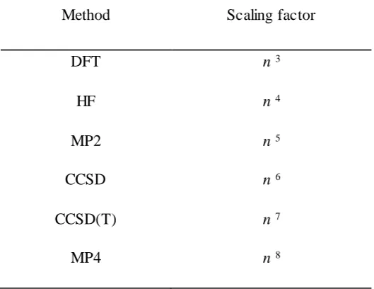
A number of methods have been developed to capture this weakness and account the electron correlation energy of a given system. These are collectively referred as post Hartree-Fock methods which includes theories such as configuration interaction (Cl), coupled cluster (CC), Møller–Plesset perturbation theory (MP2, MP3, MP4…), and multi-configurational self-consistent field (MCSCF). However, these methods are computationally expensive particularly for TM systems where a large number of electrons exist, resulting in a significant correlation energy. Additionally, these methods limited the size of system as the wavefunction depends on four variables for each electron; three spatial variables and one spin variable. Table 2.1 shows how the computational expense of different quantum mechanics methods scale, in terms of computational cost, depending on the number of electrons n.

Method Scaling factor

DFT n3

HF n4

MP2 n5

CCSD n6

CCSD(T) n7

MP4 n8

[image:42.595.187.452.472.676.2]

tp

(43)

38

Table 2.1 shows why methods that scale more favorably with systems size, such as density functional theory (DFT), have become more popular and attractive in last decades. In this work all the quantum mechanics calculations have been done using DFT. Therefore, the following section will consider DFT, including some developed approximations associated with it, such as the local density approximation 4_{and the} gradient corrected approximation (GGA).2

2.2.3 Density Functional Theory (DFT)

DFT and HF approaches are both considered as independent particle models. However, DFT considers the correlation of one electron against the electron density, whereas HF considers the correlation of one electron against an average potential of all electrons interactions within a given system in purpose of obtaining the correlation energy. Therefore, for large systems, such as transition metal systems, HF method fails to account correctly for electron correlation. For this reason DFT has become more attractive especially for a large systems such as TM-based solids and MOFs which contains many atoms and electrons.

(44)

39

kinetic energy of the system, and Ѵ describes the external potential acting on the system,

E[ρ] = T[ρ] + Ѵen [ρ] + Ѵee [ρ]. (2.5)

In addition, under the Born-Oppenheimer approximation the interactions between nuclei is constant which can be added later. T[ρ] is the kinetic energy, Ѵen [ρ] is the nucleus-electron potential energy, and Ѵee [ρ] is electron-electron potential energy. The latter can be divided into two contributions, the coulomb energy, J[ρ], and the exchange-correlation function, Exc[ρ],

E[ρ] = T[ρ] + Ѵen [ρ] + J[ρ] + Exc[ρ]. (2.6)

However, the nucleus-electron potential energy function, is known exactly, whereas the kinetic energy function and the exchange function, are unknown. Moreover, the unknown terms are not so easily derived. Equation (2.6) is known as

Thomas-Ferim-Dirac (TFD) model, which is consider as one of earliest approximations to derive the kinetic energy. However, this approximation is based on deriving the kinetic energy using the free uniform electron gas which means the orbitals and the bonding between molecules are not considered. This leads to a very poor representation of the kinetic energy.

(45)

40

electrons are treated as non-interacting electron with the same density and, therefore, the kinetic energy can be described in terms of a Slater determinant of molecular orbitals, ϕ !,

 



_

N





S

T

!

! 2 !

2

1 _





_{. (2.7)}

This can provide a correct solution to the Schrödinger equation and gives the exact kinetic energy functional which depends merely on the density. However, this approach requires the exact density which is not known. Therefore, the ground state electron density can be represented by a set of one-electron spatial orbitals (Equation 2.8)

 

2

! !



_ _



n

r





. (2.8)

Although this approach does not give an absolute answer, it is considered as one of most useful methods in modern quantum chemistry. The remaining kinetic energy along with the exchange function is incorporated into the exchange-correlation function and the Kohn-Sham DFT energy can be represented as,

(46)

41

Expanding the orbitals terms, ϕ !, for a one electron basis set leads to solution of the Kohn-Sham equations in a self-consistent manner to yield the optimum set of orbitals and hence the optimal electron density,

 

2

 

1 !

 

1 ! !

 

1

2 1 2 1 2 r d 2 1 r r r r r r r _xc en

ν





 

            





. (2.10)

The challenge of the above equation is to find the exact functional form of the exchange-correlation energy which in principle would give the exact energy from DFT. However, Exc is usually approximated and a number of different methods to

account the exchange-correlation functional are developed and will be explained briefly in the following sections.

2.2.4 The Local Density Approximation

The local density approximation is the simplest methods for approximating the exchange-correlation energy, Exc. This method assumes that Exc can be expressed in a

terms of uniform electron gas based on the density ρ(r) at a given point in the system (Equation 2.11).



( )



dr )

(r r

E

xc

(47)

42

The

ԑ

xc (ρ(r)) represents the exchange-correlation energy associated with an electron

in a uniform electron gas of density ρ(r). The exchange contribution of a uniform electron gas is given by the Dirac formula,

3 3 ( )

4 3

 

LDA r

x  . (2.12)

Additionally, the correlation energy functional has been interpolated analytically by schemes developed by Vosko, Wilk, and Nusair.7_{Although the LDA approximatio n} gives reasonable results in calculating geometries and vibrational frequencies, it gives large errors in energies. The reason behind this is the lack of the exchange and correlation energy estimations which can be corrected by implementing the generalized gradient approximation.

2.2.5 The generalized gradient approximation

The generalized gradient approximation (GGA) can be implemented to improve upon LDA. In fact, the true electron density of a system is not a homogeneous electron gas which requires a realistic method to describe the exchange-correlation energy correctly. Therefore, the inhomogeneity of the electron density can be accounted for by including its gradient, which leads to significant improvements over LDA.

(48)

43

dr r s

F E

EGGA_X  LDA_X 

 

( ) 43( )

   . (2.13)

F represents the exchange functional which can take a range of functional forms, including those with empirical parameters such as Becke’s functional.8_Moreover,_S_σ

represents the reduced density gradient which can be described by the equation below (Equation 2.14).

) (

3 4

r r S

  

 



 . (2.14)

(49)

44

2.3 Molecular Mechanics (MM)

In the Molecular Mechanics (MM) approach a system is treated classically as a collection of weights connected to each other by springs that obey simple mathematical rules such as Hooke's law. In this method, the positions of the atoms of a chemical system are determined by forces between them, including bonded and non-bonded terms. The total energies obtained from these forces are linked to the positions of the nuclei in the system leading to enforce the entire molecular structure. However, using

MM treatment for specific systems requires a suitable and flexible force field (FF). The FF is set of functions parameterized by terms such as the force constant, the ideal bond length, the ideal bond angle, etc. The values of these terms can be obtained either experimentally or theoretically, using spectroscopy data like the infrared spectrum or QM methods, respectively. Once a force field has been chosen for a particular system, the MM local optimization would be able to find the optimized geometry of that system.

(50)

45

According to Comba et al,9_{the conventional molecular mechanics method defines the} strain energy Utotal that generally arises from the total bond deformation energy (∑Eb),

the total bond angle bending energy, (∑Eθ), the total dihedral angle energy (∑Eɸ), and

the total nonbonded energy (∑Enb) consisting of van der Waals (vdW) and electrostatic

interactions (Equation 2.15).

Utotal = ∑Eb + ∑Eθ + ∑Eɸ + ∑Enb (2.15)

Each energy term is calculated mathematically using simple functions such as there shown below in equations 2.16 – 2.20,

Eb = 1

2 kb (rij – r0)2 (2.16)

where kb is the force constant and r0 is the ideal bond length. Similar way can be used

to model valence angles,

Eθ = 1₂ kθ (θijk – θ0)2 (2.17)

where kθis the strength of holding the angle at θ0 which represents the angle ideal

value. However, since a periodic function is required to model dihedral angles, the Eɸ

can be defined as,

(51)

46

where kɸ is the strength barrier value to rotate about ɸijkl which is the torsion angle.

ɸoffset presents the offset of the lowest energy from a staggered arrangement. The

non-bonded interactions, Enb, are calculated based on a function that includes an attractive

and repulsion components,

Enb = Ae –Bdij – C dij-6 (2.19)

where dij represents the distance between the two nuclei, and A, B, and C are constant

values based on Lennard-Jones vdW parameters.

In addition, Comba et al states that a number of energy terms can be added to the potential energy expression such as out – of – plane deformation Eδ and electrostatic

interactions Eε to model aromatic or sp2_{hybridized systems and the interaction of} metal complexes with biological systems respectively. The Eδ function can be

expressed as,

Eδ = 1₂ kδ δ2 (2.20)

Where kδ is the force constant and δ is the angle between the centre of plane of three

atoms bonded to a fourth atom. The electrostatic interactions are based on Coulomb law and expressed as,

(52)

47

where ε is dielectric constant, dij is the interatomic separation, and qi qj are the partial

charges on i and j atoms.

Combined with a suitable empirical parameters, these potential energy terms define the force field (FF). However, some complicated FFs are based on more complex functional forms than the harmonic oscillator expression for bond length deformation. This function can be replaced by simpler function such as a Morse function, E Morse,

for describing bond stretching (Equation 2.22).10_{Additionally, some FFs add terms} for better describing conformational and vibrations energies. For example, the Merck molecular force field (MMFF) which used the stretch-bend cross terms, Estb (Equation

2.23).11

 



e



D

EMorse 1 arr0 2 (2.22)





_

_















k j i ijk jk jk kji ij ij ijk

stb

k

r

k

r

E

, , , 0 , 0 ,

0



_(2.23)

(53)

48

molecules, such as MMFF 12-14_{, and for large biomolecules like DNA and proteins,}

such as AMBER 15_{and CHARMM}16_{. Fortunately, these force field can be revised to} increase their applicability and cover more chemical systems, including TM systems.

2.3.1 Shortcomings of MM for TM systems

The conventional MM method has been used widely in carbon chemistry which has

(54)

49

Figure 2.2; Angles bending of central atom for different common geometries.

However, a number of ingenious MM methods have been created to capture the angular geometry of metals centres in coordination compounds such as SHAPES 17 and VALBOND 18_{. MOMEC is another ingenious approach proposed by Comba et} al.8_{It deals with the angle bending of coordination compounds by employing the} ligand-ligand repulsion method analogous to points on a sphere (POS).19 Consequently, the reference θ0 values are not required. Deeth et al.20 have followed

[image:54.595.192.452.83.333.2]

(55)

50

has proven its ability to represent the angular geometries around the metal centres correctly, and gives an accurate value of the strain energy for various TM complexes. Since this work considers zinc (Zn+2_{) and copper (Cu}+2_{) containing MOF systems, all} the MM calculation are based on the LFMM method. Therefore, the following section will provide a detailed description of LFMM method.

2.3.2 Ligand Field Molecular Mechanics

Ligand field molecular mechanics (LFMM) approach is considered as one of the most effective solutions for the d-orbital effect problems. The LFMM model incorporates the ligand field stabilization energy (LFSE) directly into the potential energy expression of conventional MM,

Utotal=∑Eb + ∑Eθ + ∑Eɸ + ∑Enb + LFSE. (2.24)

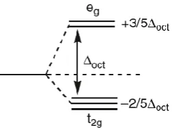
This approach uses the concept of LFSE to account for d-electrons effects, which have a significant impact on reactivity and structure of TM complexes. For example, the effect of the LFSE was proven by the experimental hydration enthalpies for hexaaqua complexes of divalent first row metal ions (Figure 2.3).22_{The typical “double hump”} behaviour shown in figure 2.3 is usually rationalized in terms of the LFSE function which can provide the d configuration and the magnitude values of the ligand field splitting, Δoct (Figure 2.4). However, these values can be corrected experimentally using the spectroscopic Δoct data giving a remarkably smooth line as shown in figure

(56)

51

Figure 2.3; Experimental hydration enthalpies values from Ca2+_(d0_{) through to Zn}2+_(d10_).

The open circles expressed the values once the effects of LFSE are removed.

Figure 2.4; Octahedral (Oh) d-orbital splitting diagram.

[image:56.595.257.383.426.521.2]

(57)

52

coordination complexes, the LFT has provided a useful picture of metal-ligand bonding in such complexes. Therefore, Deeth et al, have added the LFT model to the conventional MM to propose the ligand field molecular mechanics (LFMM) approach.1

The angular overlap model (AOM) of Schaeffer and Jorgensen 23_{is used within} LFMM to capture the LFSE. This model is a bond centred approach and assumes the total ligand field potential, ѴLF, to be the sum of the M-L bonds contributions. Each

bond can be modelled individually by AOM parameters which can be derived from spectroscopic data of the d-d splitting or theoretical studies to describe separate σ and π interactions as shown in the figure 2.5 below.

Figure 2.5; Introduction of AOM parameters of local M-L bonding showing the differences between σ and π interactions.

(58)

53

the ligands regardless their symmetries. For example, in high-symmetry geometry such as the octahedral, Oh, the splitting Δoct is expressed by equation 2.20, and illustrated for more clarity in Figure 2.6.

Δoct = 3eσ – 4eπ (2.20)

Figure 2.6; Comparison between CFT barycentre (left) and AOM barycentre (right) in case of a π-donor ligand where eπ is positive.

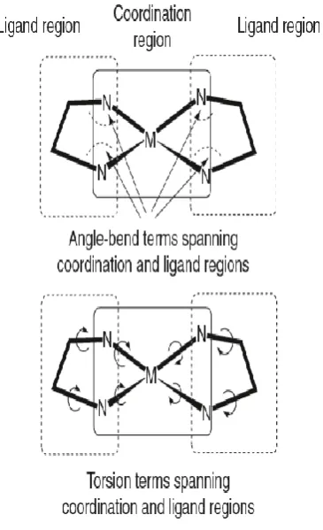
Furthermore, LFMM requires additional parameters over conventional MM to be applicable to TM complexes. The conventional MM is mainly responsible for computing organic parts, and the LFSE for the metal centre is treated by AOM approach (Figure 2.7). Since the LFSE is only computed for the d electrons effects, the M-L stretching and L-M-L angle bending terms must be included in the force field. Therefore, Deeth et al, have followed Comba et al, and used the Morse function and the ligand-ligand POS terms to describe the M-L stretching and L-M-L angle bending respectively. However, unlike Comba’s MM/AOM method,24_{the LFMM method}

(59)

54

Figure 2.7; Schematic representation of ligand and coordination regions and force field terms which represent them.

2.4 Molecular Dynamics

[image:59.595.229.412.96.396.2]

(60)

55

inappropriate in the case of flexible MOFs. However, modelling very large flexible systems for a long time, or carrying out virtual high throughput screening remains the province of classical simulation techniques.

In MD, the motion for a system of N atoms are described by the classical equation called the Newton equation. Under a specific thermodynamic conditions, such as constant temperature and/or constant pressure, a trajectory of a reaction can be generated. The trajectory can provide a crucial thermodynamic properties information for each atom which, for example, may contribute in calculating the free energy or diffusion coefficients properties. However, the MD is time-dependent approach and requires very short time (~ 1 fs) to avoid numerical instability which leads to strong limitations on the total simulation time. Nevertheless, classical MD is still the valuable approach to compute the dynamical behaviour of large systems, whether flexible or not, such as MOF and biomolecules systems for any appreciable length of time.