Perfect powers that are sums of consecutive like powers

(1)

warwick.ac.uk/lib-publications

A Thesis Submitted for the Degree of PhD at the University of Warwick

Permanent WRAP URL:

http://wrap.warwick.ac.uk/95153

Copyright and reuse:

This thesis is made available online and is protected by original copyright.

Please scroll down to view the document itself.

Please refer to the repository record for this item for information to help you to cite it.

Our policy information is available from the repository home page.

(2)

Perfect Powers that are Sums of Consecutive Like

Powers

by

Vandita Patel

Thesis

Submitted to the University of Warwick

for the degree of

Doctor of Philosophy

Mathematics Institute

(3)

Mathematics is the queen of the sciences and number theory is the queen of mathematics.

(4)

Acknowledgments

“Words fail me and tears flood to

my eyes as I attempt to express my

gratitude to and admiration for my

legendary supervisor Samir Siksek,

without whom I would still be at

Canary Wharf fiddling with excel

spreadsheets.”

SS

My most sincere gratitude goes to my supervisor, Professor Samir Siksek, for

initially inspiring me with the wonders of Number Theory, Diophantine equations

and the p-adic world during my undergraduate years. Such was this inspiration

that I could not bear to stay in the soul–less world of banking. Thank you for your

guidance, patience, support and most importantly, brilliant sense of humour and

giving me a second chance with mathemagics. �

I am highly indebted to my collaborators, Professor Mike Bennett and

Pro-fessor Samir Siksek, for introducing me to the work of Dr. Zhongfeng Zhang, which

this thesis stems from. May we continue to have many fruitful collaborations!

With Samir and Mike in Turkey at one of my first conferences, during one of

the excursions, I decided to chase The Peckin1 up a hill; fascinated by its feathered

feet. Thankfully, Samir came chasing after me, and just in time too. At the top of the

hill was the farmer wielding his shotgun! Seriously, thank you for keeping me alive

for four years, along with the support of many many friends and colleagues along

the way. Not only in Turkey, but needing medical care in Sarajevo and Bordeaux

(just to name a few - there are far too many instances of ‘Van break-downs’ to list).

Special thanks must go to Samuele and Nicolas, for helping me to get o↵the plane

when coming back to England for my defence - a memory that none of us will ever

forget!

A special mention goes to Dr. Adam Harper, who thoroughly read a

pre-liminary draft of this thesis (in the form of the infamous “Warwick Fourth Year

Report”) and his valuable suggestions helped to shape this thesis.

1_{A breed of chicken that walks like a penguin.}

(8)

Special thanks goes to Dr. Piper Harron, for it was her original thesis that

inspired me to inject all of my personality into mine.

A very special mention goes to Dr. Pieter Moree, for many helpful corrections

to this thesis, but most importantly, for reminding me that mathemagics should be

fun! �

I would like to thank my examiners, Dr. Damiano Testa and Dr. Haluk

S¸eng¨un for quite an enjoyable viva, for being super understanding during the viva

and allowing me to sit on the floor, for their time in reading my work and for their

many valuable improvements and corrections to this thesis.

To all of my supportive friends: Priya, Niketa, The Barclays Girls (Tasha,

Sabrina, Luisa, Charlene, Alicia and Asena), Lyn, Chris W., Samuele, Heline, C´eline,

Kabs, Matt B., Milena, Mirna, Shu Ting, Peter K., Mike S., George T., George K.,

Mark B., Alejandro, Lilit and Alexandre - for their brilliant company, delicious

teatimes (with wa✏es, crepes cakes and muffins, and the infamous mango

cheese-cake) and great humour.

I am much obliged to the Engineering and Physical Sciences Research Council

(EPSRC), the Max Planck Institute for Mathematics in Bonn and the Warwick

Mathematics Institute for their financial support during my time as a PhD student.

I extend my gratitude to the friendly sta↵(especially to Carole and Rimi at Warwick

and Cerolein and Svenja at MPI), PhD students and the Number Theory group at

both institutions.

Ultimately, this thesis would not have been written without the love,

en-couragement and moral support of my family. To my mother, Priti, and brother,

Dipesh, for their unconditional love. To my dearest Pravin; for always listening to

my muddled mathematical thoughts, for making many cups of tea precisely at the

moments when they are most needed, for the random spontaneous hugs and kisses

and unlimited love.

This thesis was typeset with LA_{TEX 2"}2 _{by the author.}

2_L_A

(9)

Declarations

The results presented in Parts I and II are, to the best of the author’s knowledge,

entirely new, unless otherwise stated. Many of these results have now been accepted

for publication (see Bennett et al. [2017] and Patel and Siksek [2017]).

Part I is based on collaborative work with Professor Michael A. Bennett

(University of British Columbia, Vancouver, Canada) and Professor Samir Siksek

(University of Warwick, England), which has now been published (see Bennett et al.

[2017]).

Part II is based on collaborative work with Professor Samir Siksek (University

(10)

Abstract

This thesis is concerned with finding integer solutions to certain Diophantine

equations. In doing so, we will use a variety of techniques. Unfortunately, we are not

able to mention all of them - there are many techniques in solving Diophantine

equa-tions! Combining analytic methods with classic and modern algebraic approaches

proves fruitful in a number of cases.

Our focus will be on the following Diophantine equation:

(x+ 1)k+· · ·+ (x+d)k=yn, x, y, n, d, k2Z, d, k, n 2, (|)

For fixed integers d and k, we would like to determine all of the integer

solutions (x, y, n).

Euler noted the relation 63 = 33+ 43+ 53 and asked for other instances of

cubes that are sums of consecutive cubes. Similar problems have been studied by

Cunningham, Catalan, Genocchi, Lucas and Pagliani.

Using only elementary arguments, Cassels [1985] and Uchiyama [1979]

inde-pendently solved equation (|) in the casek=d= 3 and n= 2.

Stroeker [1995] considered equation (_|) in the case k= 3, 2_d_50 with n = 2. He determined all squares that can be written as a sum of at most 50

consecutive cubes.

Zhang [2014] solved equation (|) for k 2 {2,3,4}, d = 3 and n 2 using Frey–Hellegouarch curves and the modular method. These two considerations play

(11)

In Part I of this thesis, we generalise Stroeker’s and Zhang’s work by

deter-mining all perfect powers that are sums of at most 50 consecutive cubes (see Bennett

et al. [2017]). We solve equation (_|) in the case k= 3, 2_d_50 andn 2. Here is an example of a sum of 49 consecutive cubes that is again a cube:

2913+ 2923+ 2933+ 2943+...+ 3373+ 3383+ 3393 = 11553.

Our methods include: descent, linear forms in two logarithms, sieving and

Frey-Hellegouarch curves.

In Part II of this thesis, we let k 2 be an even integer and r a non-zero

integer. We show that for almost all d 2 (in the sense of natural density), the

equation

xk+ (x+r)k+_{· · ·}+ (x+ (d 1)r)k=yn, x, y, n₂Z, n 2,

has no solutions (see Patel and Siksek [2017]). The techniques employed here are

vastly di↵erent to those used in Part I. We move away from solving individual

equations and instead present a result which shows the general behaviour of these

equations. Our main considerations are the Bernoulli polynomials, their 2-adic

(12)

Chapter 1

Diophantine Equations

“What day is it?” asked Pooh. “It’s today” squeaked Piglet. “My favourite day”, said Pooh.

Winnie the Pooh, A. A. Milne

Our journey begins in Ancient Greece, where Diophantus of Alexandria is erratically writing his series of Arithmetica. Little does he know at this stage that his collective works will become infamous. Our mysterious Diophantus is compiling problems and in some instances, even providing the solutions! He wants to find all integer solutions to certain algebraic equations. Problems such as these are nowa-days calledDiophantine equations, named aptly after him. Typically, Diophantine equations have integer coefficients and we seek only integer solutions.

Information and insight into the life of Diophantus is sparse. Our alluding mathematician is believed to have existed around 201–299 AD. Within his mathe-matical puzzles and riddles, he did leave behind clues to decipher his age1:

‘Here lies Diophantus,’ the wonder behold. Through art algebraic, the stone tells how old: ‘God gave him his boyhood one-sixth of his life, One twelfth more as youth while whiskers grew rife;

And then yet one-seventh ere marriage begun; In five years there came a bouncing new son.

Alas, the dear child of master and sage

After attaining half the measure of his father’s life chill fate took him. After consoling his fate by the science of numbers for four years, he ended his life.’

1_{Rumour has it that Metrodorus collected such mathematical epigrams and wrote very few of}

them. Perhaps Diophantus himself wrote this particular riddle, in which case this cannot be his true final age. Unfortunately, there are no current sources available to verify the age of Diophantus and I am afraid that I will have to leave you in suspense.

(13)

Many of the books in the seriesArithmeticahave been lost or destroyed and only a few managed to survive. Pierre de Fermat (1601–1665 AD) was a French jurist who extensively studied the works of Diophantus, often daydreaming about Diophantine equations during trials. He was obsessed. He is notably famous for writing in the margin of the 1621 edition of Arithmetica (written by Bachet):

“If an integer n is greater than 2, then an₊_bn ₌ _cn _{has no solutions in} non-zero integers a, b, and c. I have a truly marvelous proof of this proposition which this margin is too narrow to contain.”

Crowned Fermat’s Last Theorem despite not being even close to a theorem (this was a conjecture at the time since Fermat had notactuallyprovided a proof), Fermat’s missing proof eluded amateur and professional mathematicians alike for over 350 years!

Fermat’s Infinite Descent

Fermat himself proved that there are no integer solutions whenn= 3 orn= 4 (as did Euler independently but much later) using a very clever trick: Fermat’s method of infinite descent. Using an elementary factorisation argument, Fermat showed that if there is a solution then there also exists a smaller solution. Thus if we start out with a minimal solution then we obtain a contradiction.

The case n= 5

Dirichlet (1828) and Legendre (1830) provided a proof for the case n = 5. Legendre’s method of proof is attributed to Marie–Sophie Germain, who was unjustly mentionedonlyin the footnote!

The work of amateur mathematician, Sophie Germain, provided the first major breakthrough in the history of the Fermat equation. With a single theorem, she was able to solve the Fermat equation for manyvalues of n. Previously, many other mathematicians had contributed to the e↵ort with solutions foronlyindividual values ofn; Stewart and Tall [2016] contains an extensive history.

Sophie Germain: Rebel Mathematician

(14)

Her sudden desire to pursue the mathematical sciences was immediately met with resistance, both from family and friends as well as society. Her parents were concerned with her “abnormal” behaviour, punishing her even. Yet young Sophie was undeterred and she would often work late into the night. Her parents would confiscate her candles, clothing and even heating to deter her. Despite this, Sophie continued to work on mathematics, wrapping herself in bed linen and writing deep into the night while the ink slowly froze in it’s well.

In 1794, L’´Ecole Polytechnique opened in Paris, a perfect place for Sophie to study mathematics further. However, one caveat existed: the institute did not admit women. Taking on the identity of a former student who had left Paris, Sophie managed to enrol at the college. She continued to take on this identity for most of her career, including all correspondences between herself and prominent mathematicians of the time.

Writing under the alias of “Auguste Antoine LeBlanc” she provided a proof to Fermat’s Last Theorem, (under the assumption that n does not divide a, b or c) for all values of n _ 100. Actually, her methods were readily applicable to all n197. For at least a century after Germain, mathematicians were adapting her methods to reach contradictions for the Fermat equation for very large values ofn. Here are a few of the milestones reached in the history of the Fermat equation.

• 1823 – S. Germain;n100 and n197.

• 1908 – L. E. Dickson;n7,000.

• 1976 – S. S. Wagsta↵;n125,000.

• 1988 – A. Granville and M. Monagan;n714,591,416,091,389.

In Part I, Chapter 7, we will revisit and adapt Germain’s method to arrive at contradictions for the majority of our equations.

Bounding n

(15)

When Baker’s theory is applicable, it usually produces colossal bounds. The question of interest has now changed: do we have computational power to carry out thefinite computation?

In Part I, Chapter 3, we explore Baker’s method and a direct application to our equations show very clearly how large these bounds can be. In Part I, Chapter 6, refinements of Baker’s method for linear forms intwologarithms, given by Laurent [2008] yield more manageable bounds forn.

Proof of Fermat’s Last Theorem: There are no non-trivial solutions! The proof to the elusive Fermat’s Last Theorem came in 1995, when Wiles announced his complete proof. The argument did not build on any of the previous work and attempts that I have outlined above. A completely di↵erent approach was used, and the story for this work begins in 1975, when Yves Hellegouarch associated Elliptic curves to equations like an+bn = cn. His focus was not on the Fermat conjecture and it was only in 1982 that Gerhard Frey made the connection between this curve and the Fermat equation. Frey noticed that the curve constructed (and its modp representation) has some very special properties. Soon thereafter, Serre formulated a precise conjecture which implies Fermat’s Last Theorem. Ribet [1990] proved enough of this conjecture to show that Fermat’s Last Theorem follows from the famousTaniyama–Shimura conjecture. The Taniyama–Shimura conjecture (also called the modularity conjecture) was proved by Wiles [1995] for semistable elliptic curves, which was enough to prove Fermat’s Last Theorem. This circle of ideas gave rise to themodular method for attacking Diophantine equations, which will be crucial for us in Chapter 8.

Algorithm to Solve all Diophantine Equations?

The methods used by Diophantus to solve algebraic equations are somewhat ad-hoc. One may be able to work through 100 of his problems, yet will not be able to use the methods developed to solve the next problem. In this introduction, we have listed many di↵erent approaches to studying Diophantine equations, but I believe that we have barely scratched the surface - there are many more methods which I have not included in my exposition! This leads us to question whether it is possible to find a uniform method to determine all of the solutions to any algebraic equation, preferably a method that terminates in a finite number of steps (called an algorithm)? This was indeed the essence of Hilbert’s tenth problem, which states:

(16)

in rational integers.”

In 1970, Yuri Matiyasevich answered Hilbert’s question in the negative: no such algorithm can exist. However, there is hope to find algorithms, or structured methods to solve large families of Diophantine equations - this notion is explored in Part I of this thesis.

Given that one single sole method does not exist makes research in Dio-phantine equations remarkably alluring, bewitching, captivating, dazzling and ex-hilarating (and rather frustrating2 at times too!) for both mathematicians and non-mathematicians. There is always room and scope for the development of new methods and techniques!

1.1 This Thesis - Structure and Navigation

This thesis is organised in two parts, each with its own self-contained introduction that also contains a detailed review of the literature. Part I, uses a variety methods in solving Diophantine equations to answer the question: when is a sum of at most 50 consecutive cubes a perfect power? Part II looks at the question: when is a sum ofd consecutive powers a perfect power. The flavour and style of mathematics is vastly di↵erent to that in Part I. We move away from solving individual equations and instead, provide rigour to the notion that when one is looking for integer solutions where the exponents of the consecutive integers are even, solutions are rare.

Part I

We consider the equation

(x+ 1)3+ (x+ 2)3+· · ·+ (x+d)3 =y` x, y, `, d2Z, ` 2 (1.1)

and we are interested in finding all integer solutions (x, y,`) when 2_d_50. We can work under the assumption that ` is prime, and are able to recover solutions for any integer`from our table of solutions which shows solutions for prime3 values of `. We recover the solutions of Stroeker [1995] when `= 2. Surprisingly, we also unearth five brand new non-trivial solutions when` = 3, as well as recovering the

2_{The A–B–C–D–E–F of Diophantine Equations. Notice the imbalance in feelings?}

3_{There are no further solutions for composite values of}_`_{in our table, which only shows solutions}

whenx 1. However, solutions with composite`do appear when considering any integer valuex, for example 13_{+ 2}3₊

· · ·+ 83_{= 36}2 _{= 6}4_{. We explain how to obtain solutions for any value of}_x

(17)

solution of Euler, 33_{+ 4}3_{+ 5}3_{= 6}3_{. This part of the thesis is based on the published} work Bennett et al. [2017].

In order to find all of the integer solutions, we first obtain an upper bound for our exponent `. This leaves us with a finite number of equations, whereby we begin the process of discarding equations when they do not have a solution. Once we are left with a handful of equations, we can then determine all of the solutions.

Table 1.1 outlines the methodology used to discard equations, with a count for the number of equations remaining to be solved. We include references for the relevant chapters of Part I, so if you are interested in a particular methodology, then this has been hyperlinked for fast access (I know how eager everyone is to start solving 200 million equations - see Chapter 7)!

Chapter Methods used to Solve Equation (1.1) Number of Equations to Solve

2 Useful equations and identities 49 equations in (x, y,`)

3 `= 2: Integer points on elliptic curves 49 equations in (x, y)

4 d= 2: Results of Nagell 2 equations in (x, y,`)

5 First descent: a factorisation for` 5 906 equations in (x, y,`) 6 Linear Forms in two logarithms: ` 5 906_⇥216814 = 196,433,484

Bounding `<3_⇥106 _{equations in (}_{x, y}₎ 7 Sophie-Germain type criterion (caser ₆=t)

879⇥216814 = 190,579,506 in (x, y) 224 remain in (x, y) 8 Modularity4 _(case_r ₌_t₎

27⇥216814 = 5,853,978 in (x, y) 53 remain in (x, y) 5.3 First descent when`= 3 942 equations in (x, y)

Equations remaining via 5.3, 7 and 8 1219 remain in (x, y)

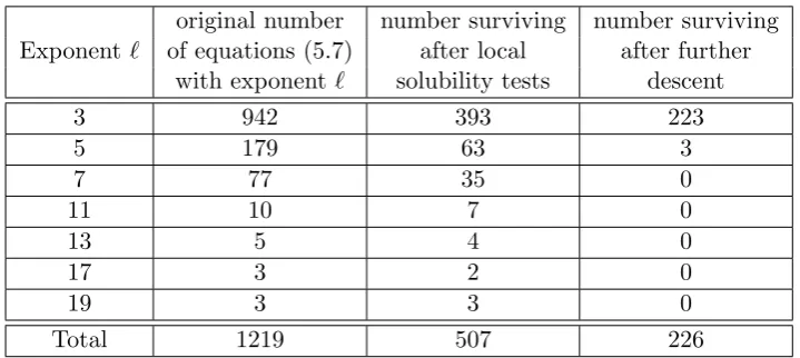
9.1 Local solubility tests 507 remain in (x, y)

9.2 A further descent 226 remain in (x, y)

[image:17.595.123.537.303.622.2]

10 Thue solver! 6 solutions found!

Table 1.1: Tracking the Number of Equations to Solve

4_{We put 27 out of the 906 equations through the modular method. In theory, we could put all}

(18)

Part II

We study the equation:

xk+ (x+r)k+_{· · ·}+ (x+ (d 1)r)k=yn, x, y, n₂Z, n 2 (1.2)

and we give density results for the solutions of this equation whenk is any positive even integer. Loosely speaking, we show that if you were to choose a value of d from the natural numbers at random, then there is 100% chance that the equation has no integer solutions. In Part II, we provide rigour to this notion, along with the relevant background material. This part of the thesis is based on the published work Patel and Siksek [2017].

(19)

Part I

(20)

Chapter 2

Introduction

— When shall we three meet again? In thunder, lightning, or in rain? — When the hurlyburly’s done, when the battle’s lost and won.

Shakespeare, Macbeth

Euler, in his 1770Vollst¨andige Anleitung zur Algebra [Euler, 1770, art. 249], notes the relation

63 = 33+ 43+ 53, (2.1)

and asks for other instances of cubes that are sums of three consecutive cubes. Dickson’sHistory of the Theory of Numbers gives an extensive survey of early work on the problem of cubes that are sums of consecutive cubes [Dickson, 1971, pp. 582–585], and also squares that are sums of consecutive cubes [Dickson, 1971, pp. 585–588] with contributions by illustrious names such as Cunningham, Catalan, Genocchi and Lucas. Both problems possess some parametric families of solutions; one such family was constructed by Pagliani [1829/30]:

✓

v5+v3 2v 6 ◆3 = v3 X i=1 ✓

v4 3v3 2v2 2

6 + i

◆3

, (2.2)

where the congruence restrictionv⌘2 or 4 mod 6 ensures integrality of the cubes. Pagliani constructed this paramteric family in response to a challenge (posed in the same journal) of giving 1000 consecutive cubes whose sum is a cube. Of course, the problem of squares that are sums of consecutive cubes possesses the well-known parametric family of solutions

✓

d(d+ 1) 2 ◆2 = d X i=1 i3=

d

X

i=0 i3.

(21)

that the only square expressible as a sum of three consecutive positive cubes is

62 = 13+ 23+ 33. (2.3)

Independently, both Cassels [1985] and Uchiyama [1979] determine the squares that can be written as sums of three consecutive cubes (without reference to Lucas) showing that the only solutions in addition to (2.3) are

0 = ( 1)3+ 03+ 13, 32 = 03+ 13+ 23, 2042 = 233+ 243+ 253. (2.4)

Lucas also states that the only square that is the sum of two consecutive positive cubes is 32 _{= 1}3₊₂3_{and the only squares that are sums of 5 consecutive non-negative} cubes are

102 = 03+ 13+ 23+ 33+ 43, 152= 13+ 23+ 33+ 43+ 53,

3152 = 253+ 263+ 273+ 283+ 293, 21702 = 963+ 973+ 983+ 993+ 1003,

29402 = 1183+ 1193+ 1203+ 1213+ 1223.

These two claims turn out to be correct as shown by Stroeker [1995]. In modern language, the problem of which squares are expressible as the sum ofdconsecutive cubes, reduces for any given d 2, to the determination of integral points on a genus 1 curve. Stroeker [1995], using a (by now) standard method based on linear forms in elliptic logarithms, solves this problem for 2_d_50.

The problem of expressing arbitrary perfect powers as a sum ofdconsecutive cubes withdsmall has received somewhat less attention, likely due to the fact that techniques for resolving such questions are of a much more recent vintage. Zhongfeng Zhang [2014] showed that the only perfect powers that are sums of three consecutive cubes are precisely those already noted by Euler (2.1), Lucas (2.3) and Cassels (2.4). Zhang’s approach is to write the problem as

yn= (x 1)3+x3+ (x+ 1)3 = 3x(x2+ 2), (2.5)

and apply a descent argument that reduces this to certain ternary equations that have already been solved in the literature.

(22)

consecutive cubes that is again a cube:

2913+ 2923+ 2933+ 2943+· · ·+ 3373+ 3383+ 3393= 11553.

We easily verify that this solution (or indeed any of the other solution for`= 3 that is not Lucas’ identity) does not belong to Pagliani’s family simply by checking that the equation (or amended equation)

v5+v3 2v

6 = 1155

has no rational solutions.

2.1 The Results

In this part of this thesis, we consider the equation

(x+ 1)3+ (x+ 2)3+_{· · ·}+ (x+d)3 =y`, x, y, `, d₂Z, d, ` 2.

We extend the work of Stroeker [1995] and determine all perfect powers that are sums of d consecutive cubes, with 2 _ d _ 50. This upper bound is somewhat arbitrary as our techniques extend to essentially any fixed values ofd. In addition to Stroeker’s solutions for ` = 2 and Euler’s solution for ` = 3 (2.1), we find the following 5 additional solutions, all corresponding to the value`= 3.

113+ 123+ 133+ 143= 203,

33+ 43+ 53+_{· · ·}+ 223= 403,

153+ 163+ 173+_{· · ·}+ 343 = 703,

63+ 73+ 83+_{· · ·}+ 303= 603,

2913+ 2923+ 2933+· · ·+ 3393 = 11553.

Remark: The additional solutions found for `= 3 stated above cannot be derived from Pagliani’s parametric family of solutions (see equation (2.2)). Euler’s solution is part of Pagliani’s parametric family: in equation (2.2), letv= 2.

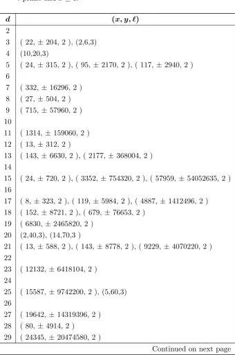
In this part of the thesis, we prove the following theorem. We expand upon the published joint paper Bennett et al. [2017] and give a full exposition.

(23)

to the equation

(x+ 1)3+ (x+ 2)3+· · ·+ (x+d)3 =y` (2.6)

[image:23.595.150.491.213.727.2]

withx 1 are given in Table 2.1.

Table 2.1: The solutions to equation (2.6) with 2d50, `prime andx 1.

d (x, y,`)

2

3 ( 22,±204, 2 ), (2,6,3) 4 (10,20,3)

5 ( 24,_±315, 2 ), ( 95, _±2170, 2 ), ( 117,_±2940, 2 ) 6

7 ( 332,_±16296, 2 ) 8 ( 27,_±504, 2 ) 9 ( 715,±57960, 2 ) 10

11 ( 1314,_±159060, 2 ) 12 ( 13,±312, 2 )

13 ( 143,_±6630, 2 ), ( 2177,_± 368004, 2 ) 14

15 ( 24,±720, 2 ), ( 3352,±754320, 2 ), ( 57959, ±54052635, 2 ) 16

17 ( 8,_±323, 2 ), ( 119, _±5984, 2 ), ( 4887,_±1412496, 2 ) 18 ( 152,±8721, 2 ), ( 679,±76653, 2 )

19 ( 6830,_±2465820, 2 ) 20 (2,40,3), (14,70,3 )

21 ( 13,±588, 2 ), ( 143, ±8778, 2 ), ( 9229,±4070220, 2 ) 22

23 ( 12132,±6418104, 2 ) 24

25 ( 15587,_±9742200, 2 ), (5,60,3) 26

27 ( 19642,_±14319396, 2 ) 28 ( 80,_±4914, 2 )

29 ( 24345,±20474580, 2 )

(24)

[image:24.595.151.495.111.509.2]

Table 2.1 – continued from previous page

d (x, y,`)

30

31 ( 29744,_±28584480, 2 )

32 ( 68,±4472, 2 ), ( 132,±10296, 2 ), ( 495,± 65472, 2 ) 33 ( 32,_±2079, 2 ), ( 35887,_± 39081504, 2 )

34

35 ( 224,±22330, 2 ), ( 42822, ±52457580, 2 ) 36

37 ( 50597,_±69267996, 2 ) 38

39 ( 110,_±9360, 2 ), ( 59260, _±90135240, 2 ) 40 ( 3275,_±1196520, 2 )

41 ( 68859,±115752840, 2 ) 42 ( 63,_±5187, 2 )

43 ( 79442,_±146889204, 2 ) 44

45 ( 175,_±18810, 2 ), ( 91057, _±184391460, 2 ) 46

47 ( 103752,± 229189296, 2 )

48 ( 63,_±5880, 2 ), ( 409,_±62628, 2 ), ( 19880, _±19455744, 2 ), ( 60039,±101985072, 2 )

49 ( 117575,± 282298800, 2 ), (290,1155,3) 50 ( 1224,_±312375, 2 )

2.2 Without Loss of Generality, let

x

1

The restrictionx 1 imposed in the statement of Theorem 2.1.1 is merely to exclude a multitude of artificial solutions. Solutions withx_0 can in fact be deduced easily, as we now explain:

(25)

(ii) For odd exponents`, there is a symmetry between the solutions to (2.6):

(x, y,`) !( x d 1, y,`).

This allows us to deduce, from Table 2.1 and (i), all solutions withx_ d 1.

(iii) The solutions with d_x _ 2 lead to non-negative solutions with smaller values ofdthrough cancellation (and possibly applying the symmetry in (ii)).

Of course arbitrary perfect powers that are sums of at most 50 consecutive cubes can be deduced from our list of`-th powers with `prime.

2.3 Some Very Important Identities

A sum ofdconsecutive cubes can be written as

(x+ 1)3+ (x+ 2)3+· · ·+ (x+d)3 =

✓

dx+d(d+ 1) 2

◆ ✓

x2+ (d+ 1)x+ d(d+ 1) 2

◆

.

Thus, to prove Theorem 2.1.1, we need to solve the Diophantine equation

✓

dx+d(d+ 1) 2

◆ ✓

x2+ (d+ 1)x+d(d+ 1) 2

◆

=y`, (2.7)

with`prime and 2d50. We find it convenient to rewrite (2.7) as

d(2x+d+ 1)

✓

x2+ (d+ 1)x+d(d+ 1) 2

◆

= 2y`. (2.8)

We will use a descent argument together with the identity

4

✓

x2+ (d+ 1)x+ d(d+ 1) 2

◆

(2x+d+ 1)2 =d2 1. (2.9)

(26)

Chapter 3

The Case

`

= 2

: An Elliptic

Curve

Tea and honey is a very grand thing.

In this section, we treat the case `= 2 separately. In this case, we are able to reduce the problem to computing integer points on Elliptic curves. Although this case has been resolved by Stroeker [1995], we provide details and some background on elliptic curves. The computational aspect is in itself interesting, and we will provide a short discussion on this topic. A secondary motivation for elongating this chapter is in order to set up the relevant notation which will be handy when it comes to discussing the modular method.

3.1 Background: Elliptic Curves

This section primarily follows [Silverman, 2009, Chapter III]. We adopt some of their notation for consistency. In this thesis, we will usually work with elliptic curves defined over the rational field, unless otherwise stated. Hence, the results in this section are stated for elliptic curves over the rational field. The results can be extended to elliptic curves over number fields and remain true with the appropriate modifications.

For us an elliptic curve E/_Q is a smooth projective curve in _P2 _{which in} affine coordinates is given by a long Weierstrass equation,

E : Y2+a1XY +a3Y =X3+a2X2+a4X+a6, (3.1)

with a1, a2, a3, a4, a6 2 Q. Remember that in projective coordinates, we still have the marked point at infinity, given projectively byO= [0 : 1 : 0].

(27)

1

2(Y a1X a3) gives us the followingmedium Weierstrass equation,

E : Y2= 4x3+b2x2+ 2b4x+b6,

where

b2 =a21+ 4a2, b4= 2a4+a1a3 and b6 =a23+ 4a6.

The Discriminant and j-invariant of an elliptic curve in medium Weierstrass form are given by

:= b2₂b8 8b34 27b26+ 9b2b4b6 and j :=c34/ ,

where

b8 :=a21a6+ 4a2a6 a1a3a4+a2a23 a24 and c4 =b22 24b4.

The smoothness of the Weierstrass model (which forms part of the definition of the elliptic curve) is equivalent to ₆= 0. The set of rational points onE is denoted by E(Q). This consists of the point at infinity, together with affine points (x, y)2Q2 satisfying the Weierstrass equation. There is a group operation onE(see [Silverman, 2009, Chapter III] for definition). This makes E(Q) into an abelian group with _O as identity; this is called the Mordell–Weil group.

Theorem 3.1.1 (Mordell–Weil). The group E(Q) is finitely generated. Thus we may write

E(Q)⇠=E(Q)tors⇥Zr

where E(Q)tors is the torsion subgroup (points of finite order, which are finite) and

r is the rank of E/Q (a non-negative integer).

For a proof of Theorem 3.1.1 see [Silverman, 2009, Chapter VIII].

3.1.1 Integer Points on Elliptic Curves

This subsection primarily follows [Silverman, 2009, Chapter IX] and we continue to adopt their notation for consistency.

(28)

1. How many integer points does E have?

2. Are there finitely many of them?

3. Can we list all of them? (i.e. perform a finite computation)

We begin this subsection with a result of Siegel that addresses question 2 and answers it positively. Siegel provided two proofs to Theorem 3.1.2 by means ofDiophantine approximation. Both proofs are ine↵ectivedue to the method used. Siegel answered yes to question 2, but neither proof gives an explicit computable upper bound for the size of such a point, called theheight. Therefore, questions 1 and 3 still remain unanswered for the moment.

Theorem 3.1.2(Siegel). There are finitely many integral points on E/_Q.

Siegel’s second proof reduced the problem of finding integer points on elliptic curves to looking for solutions of some S-unit equations. Using Baker’s theory of linear forms in logarithms in addition to Siegel’s proof provides positive answers to questions 1 and 3, with the answer to 3 being yes in theory. Baker’s theory usually churns out extremely large upper bounds for the height. We will shortly see an example of this, thus leaving us with a sense of“did we really answer question 3 in the positive?”

Theorem 3.1.3 (Baker). Let K be a number field. Let ↵1, . . . ,↵n 2 K⇤ and 1, . . . , n2K. For any constant ⌫, define

⌧(⌫) : =⌧(⌫;↵1, . . . ,↵n; 1, . . . , n)

=h([1, 1, . . . , n])h([1,↵1, . . . ,↵n])⌫.

where h is a logarithmic height function. Fix an embedding K _⇢_C and let _{| · |} be the corresponding absolute value. Assume that

1log↵1+· · ·+ nlog↵n6= 0.

Then there are e↵ectively computable constants C,⌫ >0 which depend only onn and[K :Q] such that

| 1log↵1+· · ·+ nlog↵n|> C ⌧(⌫).

(29)

3.1.2 Baker Bounds for our Consecutive Cubes

Baker’s theory gives e↵ective, yet rather large, bounds for Siegel’s theorem. We shall demonstrate by studying what happens to our consecutive cubes. For the following theorem see [Baker, 1990, page 45] or [Silverman, 2009, page 261].

Theorem 3.1.4 (Baker). Let A, B, C, D 2 Z satisfy max{|A|,|B|,|C|,|D|}  H. Assume that

E :=Y2 =AX3+BX2+CX+D

is an elliptic curve. Then any integer point P = (x, y)2Z2 _on _E _satisfies

max_{|x_|,_|y_|}<exp⇣ 106H 106⌘:=BB.

Let`= 2 in equation (2.7). We can expand the left hand side to get;

Ed : y2=dx3+ 3

2d(d+ 1)x 2₊d

2(d+ 1)(2d+ 1)x+ d2

4(d+ 1) 2_.

We can apply Theorem 3.1.4 to see what astronomical bounds we can naively ex-pect in computations. For our range, 2_ d _50, we compute the minimum and maximum values forBBthat we obtain. In this calculation we see that the smallest Baker bound obtained is still pretty huge!

d H Baker Bound

[image:29.595.215.421.456.516.2]

2 15 1.8157· · ·⇥107,176,091 50 1,625,625 2.3417· · ·⇥1012,211,020

Table 3.1: Baker Bounds

Fortunately for us, substantial help and improvement comes from linear forms in elliptic logarithmsto significantly reduce the Baker bound; see Smart [1998] for details. The method of linear forms in elliptic logarithms is implemented in

Magmaand can compute integral points on Weierstrass models, provided a Mordell–

(30)

3.2 Application: Finding Solutions!

Although Theorem 2.1.1 with`= 2 follows from Stroeker [1995], we explain briefly how this can now be done with the help of an appropriate computer algebra package. Let (x, y) be an integral solution to (2.7) with ` = 2. Write X = dx, and Y =dy. Then (X, Y) is an integral point on the elliptic curve

Ed : Y2 =

✓

X+d 2₊_d

2

◆ ✓

X2+ (d2+d)X+d 4₊_d3

2

◆

.

Using the computer algebra packageMagma[Bosma et al. [1997]], we determined the integral points onEd for 2d50. For this computation,Magmaapplies the stan-dard linear forms in elliptic logarithms method [Smart, 1998, Chapter XIII], which is the same method used by Stroeker (though the implementation is independent). From this we immediately recover the original solutions (x, y) to (2.7) with ` = 2, and the latter are found in our Table 2.1. We have checked that our solutions with `= 2 are precisely those given by Stroeker.

(31)

Chapter 4

The Case

d

= 2

: Applying the

Results of Nagell

Our method for generaldexplained in later sections fails ford= 2. This is because of the presence of solutions (x, y) = ( 2, 1) and (x, y) = ( 1,1) to (2.6) for all ` 3. In this section we treat the case d= 2 separately, reducing to Diophantine equations that have already been solved by Nagell.

4.1 Background: The Equations

X

2

+

X

+ 1 =

Y

n

and

X

2

+

X

+ 1 = 3Y

n

This section is predominantly concerned with the following theorem of Nagell which can be found in Nagell [1921]. A treatment of (4.2) can also be found in [Cohen, 2007a, pages 420–421].

Theorem 4.1.1(Nagell, 1921). The only integer solutions to the equation

X2+X+ 1 =Yn (4.1)

with n 6= 3k are the trivial ones with X = 1 or 0. The only integer solutions to the equation

X2+X+ 1 = 3Yn (4.2)

(32)

4.2 Application: Finding Solutions!

Recall equation (2.6) withd= 2 and ` 3 a prime:

(x+ 1)3+ (x+ 2)3 =y`.

For convenience, letz=x+ 1. Then, the equation becomesz3_{+ (}_z_{+ 1)}3 ₌_y`_which

can be rewritten as

(2z+ 1)(z2+z+ 1) =y`. (4.3)

Here y and z are integers and ` 3 is prime. Suppose first that ` = 3. This equation here defines a genus 1 curve. We checked usingMagmathat it is isomorphic to the elliptic curveY2 ₉_Y ₌_X3 _{27 with Cremona label}_27A1_{, and that it has} Mordell–Weil group (over Q) ⇠= Z/3Z. It follows that the only rational points on (4.3) with`= 3 are the three obvious ones : (z, y) = ( 1/2,0), (0,1) and ( 1, 1). These yield the solutions (x, y) = ( 1,1) and (x, y) = ( 2, 1) to (2.6).

We may thus suppose that` 5 is prime. The resultant of the two factors on the left-hand side of (4.3) is 3 and, moreover, 9-(z2+z+ 1).1 It follows that either

2z+ 1 =y`₁, z2+z+ 1 =y₂`, y=y1y2 (4.4)

or

2z+ 1 = 3` 1y₁`, z2+z+ 1 = 3y₂`, y = 3y1y2. (4.5)

By Theorem 4.1.1 the only solutions to equation (4.4) are the trivial ones, (z, y) = ( 1, 1) and (0,1) for any odd prime `. Working back, we recover the solutions (x, y) = ( 2, 1) and ( 1,1) for any odd prime `to (2.6).

Again by Theorem 4.1.1, the only solutions to equation (4.5) are the trivial ones, (z, y2) = ( 2,1) and (1,1). We have (z, y) = ( 2, 3) and (1,3). Working back, we do not recover a solution for the case (z, y) = ( 2, 3). We get x = 3 which gives us the following non-perfect power, ( 2)3_{+ ( 1)}3 ₌ _{9. In the case} (z, y) = (1,3) we yield a solution (x, y) = (0,3) i.e. 13+ 23 = 32. However, we are only interested in solutions where x 1 for our tables, as explained in Chapter 2. Moreover, for this section, we are under the assumption that` 3. (The case `= 2 has already been considered in Chapter 3).

Remark: In Bennett et al. [2017] we incorrectly state that equation X2 ₊_X ₊ 1 = 3Yn _for _{n >} _{2 only has the trivial solution with} _X _{= 1. There is also the}

1_{We can check that the congruence}_a2₊_a_{+ 1}

(33)

(34)

Chapter 5

First Descent for

`

3

One of the advantages of being disorganized is that one is always having surprising discoveries.

In this chapter, we perform a descent (basically a clever factorisation) for equation (2.8) when 3 _ d _ 50 and ` 3. For each value of d, we are able to perform the descent uniformly for all ` 5. By a uniform descent, we mean that all factorisations produced are independent of` 5. This step is essential in producing ternary equations in the correct format to then be amenable to techniques described in later chapters (for example, linear forms in logarithms, Sophie-Germain type methods and the modular approach).

Writing up the descent for individual values of 3_d_50 would soon become repetitive, with an extremely cluttered exposition. So instead, we get the computer to perform the descent for us. In order to get the computer to do all of the work, we first need to specifythe algorithm, which is a finite number of calculations that the computer must carry out to show us all of the possible factorisations.1

Here is a reminder of equation (2.8):

d(2x+d+ 1)

✓

x2+ (d+ 1)x+d(d+ 1) 2

◆

= 2y`.

Before we state the algorithm, we first give a concrete example to show the types of calculations that can occur.

5.1 An Example: Descent for

d

= 5

,

`

3 :

Letd= 5 and ` 5. Then equation (2.8) in this specific case is

5 (x+ 3) x2+ 6x+ 15 =y`.

1_{There are only a finite number of possible factorisations and this will be shown in the}

(35)

This can be rewritten as

(x+ 3) x2+ 6x+ 15 = 5` 1w`,

wherey = 5w. First we make a sensible change of variables. This is not necessary and indeed omitted in our algorithm, but for this specific case, it will show the key steps in our algorithm more transparently. We letz=x+ 3 to get:

z z2+ 6 = 5` 1w`.

There is an obvious factorisation to the left hand side of the equation. Therefore, we would like to know the factorisation for the right hand side. This is the main idea behinddescent.

We will need theresultantofzand z2+ 6, which is equal to 6 in this case, to determine the possible factorisations that can happen on the right hand side. The resultant tells us that the factors on the left hand side,zandz2+ 6 have a greatest common divisor (abbreviated to gcd) that is 1,2,3 or 6. We are using a key fact here: the gcd between two polynomials divides the resultant.

Notice that we have 5` 1on the right hand side. Translating this information to the left hand side, we see that either 5` 1 dividesz or it dividesz2+ 6: 5 cannot divide both z and z2_{+ 6, otherwise we contradict the information about their gcd} obtained from calculating the resultant.

We are ready to state all of the possible equations obtained from the first2 descent. We can conveniently split the cases into two: When 5_|z and when 5_-z. We let↵= gcd(z,6). Thus, ↵₂_{1,2,3,6_}.

Case 5_|z: In this case

z= 5` 1↵` 1y₁`, z2+ 6 =↵y₂`,

wherey1 and y2 are integers and w=↵y1y2.

Case 5-z: In this case

z=↵` 1y₁`, z2+ 6 = 5` 1↵y₂`,

where again y1 and y2 are integers andw=↵y1y2.

Remark: In performing the descent when d = 5, one may notice that this is completely independent of ` when ` 5. After the descent, we have a total of 8

(36)

cases, or equations, to consider. In performing the descent for all 3_d_ 50 and ` 5, we split our equation up into di↵erent cases and hence obtain 906 ternary equations to solve in the variables (y1, y2,`).3 The argument in the next section is only for` 5 and will need modification for`= 3, which we carry out in Section 5.3.

5.2 The Algorithm: A Uniform Descent for

`

5

Let d 3. We consider equation (2.8) with exponent ` 5. In this section, we determine the algorithm to perform a uniform descent for any value ofd 3 which is independent of` 5. As stated previously, the argument in this section will need modification for`= 3 which we carry out in Section 5.3.

For a primeq we let

µq = ordq(d2 1) and ⌫q= ordq(d), (5.1)

i.e. the exponent of the largest power of q dividing d2 1 and d, respectively. We associate toq a finite subsetTq⇢Z2 _{as follows.}

• Ifq-d(d2 1) then let Tq ={(0,0)}.

• Forq= 2 we define

T2 =

8 > > > < > > > :

{(0,1 ⌫2)} if 2|d

{(1,0), (µ2/2,1 µ2/2), (3 µ2, µ2 2)} if 2-dand 2|µ2

{(1,0), (3 µ2, µ2 2)} if 2-dand 2-µ2.

• For oddq |d, let

Tq ={( ⌫q,0), (0, ⌫q)}.

• For oddq |(d2 1), let

Tq =

8 < :

{(0,0), ( µq, µq), (µq/2, µq/2)} if 2|µq,

{(0,0), ( µq, µq)} if 2-µq.

We takeAd to be the set of pairs of positive rationals (↵, ) such that

(ordq(↵),ordq( ))2Tq 3_{Solving for (}_y

(37)

for all primesq. It is clear that_Adis a finite set, which is, in practice, easy to write down for any value ofd.

Lemma 5.2.1. Let (x, y)be a solution to (2.8)where ` 5 is a prime. Then there are rationals y1, y2 and a pair (↵, )2Ad such that

2x+d+ 1 =↵y`₁, x2+ (d+ 1)x+ d(d+ 1)

2 = y

`

2. (5.2)

Moreover, if3_d_50 theny1 and y2 are integers.

Remark: The reader will observe that the definition of _Ad is independent of `. Thus, given d, the lemma provides us with a way of carrying out the descent uni-formly for all` 5.

Proof. Let us first assume the first part of the lemma and deduce the second. Using a shortMagma script, we wrote down all possible pairs (↵, ) ₂_Ad for 3 d50 and checked that

max{ordq(↵), ordq( )}4 for all primesq. Asx is an integer, we know from (5.2) that

ordq(↵) +`ordq(y1) 0 and ordq( ) +`ordq(y2) 0,

for all primes q. Since ` 5, it is clear that ordq(y1) 0 and ordq(y2) 0 for all primesq. This proves the second part of the lemma.

We now prove the first part of the lemma. For 2x+d+ 1 = 0 (which can only arise for odd values of d) we can takey1 = 0, y2= 1,

↵ = 8

d(d2 ₁₎ and = d2 ₁

4 ; (5.3)

it is easy to check that this particular pair (↵, ) belongs to_Ad. We shall henceforth suppose that 2x+d+ 1₆= 0.

Claim: Letq be a prime and define

✏= ordq(2x+d+ 1) and = ordq

✓

x2+ (d+ 1)x+d(d+ 1) 2

◆

.

Then (✏, )_⌘(✏0_, 0_{) mod}_` _{for some (✏}0_, 0₎₂_T_q_.

(38)

suppose thatq_|d(d2 _{1). Observe that for any}_q_{, from (2.8),}

⌫q+✏+ ⌘ordq(2) mod `. (5.4)

Moreover, from (2.9),

µq min(2✏, + 2 ordq(2)) with equality if 2✏6= + 2 ordq(2). (5.5)

We deal first with the case where q = 2 | d (so that ✏ = 0). By (5.4), we obtain that (✏, ) _⌘ (0,1 ⌫2) mod`, and, by definition, T2 = {(0,1 ⌫2)} establishing our claim. Next we suppose thatq = 2-d(in which case ⌫2= 0):

• If 2✏= + 2 then, from (5.4) and the fact that ` 5, we obtain (✏, )⌘(1,0) mod`.

• If 2✏ > + 2 then, from (5.5), we have µ2 = + 2, so from (5.4) we obtain (✏, )_⌘(3 µ2, µ2 2) mod`.

• If 2✏ < + 2 then, from (5.5), we have µ2 = 2✏, so from (5.4) we obtain (✏, )_⌘(µ2/2,1 µ2/2) mod`.

Next, let us next consider odd q _|d (whereby we have that µq = 0). From (5.5), it follows that either ✏= 0 or = 0. From (5.4), we obtain (✏, ) ⌘(0, ⌫q) or ( ⌫q,0) mod`as required.

Finally we consider oddq _|(d2 1) (so⌫q = 0):

• If 2✏ = then, from (5.4) and the fact that ` 5, we obtain (✏, ) _⌘ (0,0) mod`.

• If 2✏ > then, from (5.5), we haveµq = , so from (5.4) we obtain (✏, ) ⌘ ( µq, µq) mod`.

• If 2✏< then, from (5.5), we have µq = 2✏, so from (5.4) we obtain (✏, ) ⌘

(µq/2, µq/2) mod`.

From (5.2) and (2.9), we deduce the following ternary equation

4 y`₂ ↵2y2₁`=d2 1. (5.6)

(39)

coefficients we can rewrite this as

ry`₂ sy2₁`=t (5.7)

wherer,s,t are positive integers and gcd(r, s, t) = 1.

5.3 The Algorithm: Descent for

`

= 3

In this section we modify the approach of Section 5.2 to deal with equation (2.8) with exponent`= 3.

For an integerm, we denote by [m] the element in{0,1,2}such thatm⌘[m] mod 3. For a primeq we letµq and ⌫q be as in (5.1). For each primeq, we define a finite subsetTq ⇢{(m, n) : m, n2{0,1,2}}.

• Ifq-d(d2 _{1) then let} _T

q ={(0,0)}.

• Forq= 2 we let

T2 =

8 > > > < > > > :

{(0,[1 ⌫2])} if 2|d

{(1,0), (0,1), (2,2)_} if 2-dand µ2 4.

{(1,0), (0,1)} if 2-dand µ2= 3.

• For oddq _|d, let

Tq ={([ ⌫q],0), (0,[ ⌫q])}.

• For oddq _|(d2 1), let

Tq =

8 < :

{(0,0), (1,2), (2,1)_} ifµq 2

{(0,0), (2,1)} ifµq= 1.

Let_Adbe the set of pairs of positive integers (↵, ) such that (ordq(↵),ordq( ))2 Tq for all primes q.

Lemma 5.3.1. Let (x, y) be a solution to (2.8) where ` = 3 a prime. Then there are integersy1, y2 and a pair (↵, )2Ad such that (5.2)holds.

(40)

5.4 Proof of Theorem 2.1.1: Descent for

`

= 3

From this lemma and (2.9) we reduce the resolution of (2.8) with`= 3 to solving a number of equations of the form (5.6). These can be transformed by clearing denominators and dividing by the greatest common divisor of the coefficients into equations of the form (5.7) wherer,s,tare positive integers and gcd(r, s, t) = 1. An implementation of above procedure leaves us with 942 quintuples (d,`, r, s, t) with `= 3.

(41)

Chapter 6

Linear Forms in Logarithms

“I don’t feel very much like Pooh today,” said Pooh.

“There, there,” said Piglet. “I’ll bring you tea and honey until you do.”

The descent step in the previous chapter transforms (2.8) into a family of ternary equations (5.6). In this section, we appeal to lower bounds for linear forms in logarithms to find an explicit upper bound for the exponent`appearing in these equations.

We have already seen an example of the application of linear forms in loga-rithm in Chapter 3, Subsection 3.1.1. This chapter requires us to use the specific case oflinear forms in two logarithms.

The first section of this chapter, Section 6.1, uses a theorem in Cohen [2007b] to give us a naive bound for`. It turns out that this bound is better than that given in Bennett et al. [2017]. The focus of the remainder of this chapter then turns to the original work by Bennett et al. [2017]. We expand on the details since the calculations are very explicit, and some of the intricate workings of linear forms in two logarithms become extremely transparent.

6.1 A Naive Bound: Linear Forms in Two Logarithms

In this section, we follow [Cohen, 2007b, Chapter 12, p. 423]. We begin by stating a theorem due to Mignotte and then apply the theorem to our ternary equations.

Theorem 6.1.1(Mignotte). Assume that the exponential Diophantine inequality

|axn byn|c, witha, b, c2Z 0 and a6=b,

has a solution in strictly positive integers x and y with max_{x, y_} > 1. Let A = max_{a, b,3_}. Then

n_max

⇢

3 log (1.5_|c/b_|), 7400 logA

(42)

Remark: If A = b and a = 1, then logA/log (_|a/b_|) = 1. Therefore, our denominator becomes log(1 1) = log(0). Since the original Diophantine inequality is _|axn _byn_|_ _c_{, we may swap the terms} _axn _and _byn_{. Appropriate relabelling} gives usA=aand b= 1 to overcome this problem.

6.1.1 Naive Bounds for our Sums of Consecutive Cubes

From the previous section, recall equation (5.7):

ry`₂ sy2₁`=t

where r, s, t are positive integers and gcd(r, s, t) = 1. The descent step of the previous section left us with a finite set of (r, s, t) tuples, which were obtained from the finite pairs (↵, ) ₂_Ad for 3d50. Checking all of the tuples (r, s, t) with Theorem 6.1.1 in Magma, we see that the maximum value of ` occurs at d = 50, where we obtain the bound:

`_986,053.

Remark: This procedure leaves us with only one exceptional tuple when d = 8 and (r, s, t) = (1,1,63) for which Theorem 6.1.1 cannot be applied (in this instance, the condition a 6=b is violated). Notice that the corresponding values of ↵ and are (1,1/4).1 _{For (}_{r, s, t}_{) = (1}_,₁_,_{63), we want to solve} _y`

2 y12` = 63. Let’s change variables and letx:=y`₁. Then we want to find all integer solutions tox2+ 63 =y₂`, which has already been solved in the literature (see Bugeaud et al. [2006]). It has solutions

(_|x_|,_|y_|,`) = (1,4,3), (13537,568,3), (31,4,5), (1,2,6), (31,2,10).

Noting that 13537 and 31 are prime, and x = y`₁, means that ` must be equal to 1. Hence, we do not yield solutions for our sum of 8 consecutive cubes in these cases. On the other hand, the solutions (1,4,3) and (1,2,6) yield essentially same solution: namely 63 = 1 + 43 = 1 + 26. Undoing the descent step that occurred in the previous chapter, we havey =↵ y1y2 = 43. Going right back to the beginning of our calculations, we are able to solve the equation (for a sum of 8 consecutive cubes being a perfect power) in the indeterminatex:

(x+ 1)3+_{· · ·}+ (x+ 8)3= 43,

(43)

where we find the solutionx= 4. Noting that our table only shows solutions when x 1, we are done.

6.2 A Result of Laurent for Linear Forms in Two

Log-arithms

In this section, we require a result of Laurent on linear forms in two logarithms of algebraic numbers. By analgebraic number we mean an element of↵₂_C, which is the root of a non-zero polynomial with rational coefficients. If we choose the non-zero polynomial inQ[x] with minimal degree, then this is irreducible, and is called theminimal polynomialof↵. The minimal polynomial is unique up to scaling, and is usually taken to be monic. In this subject (linear forms in logarithms) however, the minimal polynomial is scaled so that the coefficients are integers, but their gcd is 1. Let↵ have minimal polynomial f(x) given by:

f(x) :=adxd+· · ·+a0 = 0, ai2Z

where gcd(a0, . . . , ad) = 1 and ad 6= 0. Let ↵(i), . . . ,↵(d) be the roots of f(x) in

C; these are the conjugates of ↵. We define the absolute logarithmic height of an algebraic number↵ by:

h(↵) = 1

d log|ad|+ d

X

i=1

log max(1,|↵i|)

!

.

Definition 6.2.1. For non-zero algebraic numbers ↵ and , we say that they are multiplicatively independent if the only solution to ↵m n = 1 with m, n 2 Z is (m, n) = (0,0).

Lemma 6.2.2. If ↵ and are positive real algebraic numbers that are multiplica-tively dependent, then there are coprime integersu and v, which are not both zero, such that↵u₌ v_.

Proof. As ↵ and are algebraically dependent, there are integers m and n, not both zero such that ↵m n= 1. Letg = gcd(m, n). Let u=m/g and v= n/g, so that u and v are coprime integers and not both zero. Then we can rewrite ↵m n as (↵u_/ v₎g _{= 1. Thus} _↵u_/ v _{is a} _g_{-th root of unity. However,} _↵u_/ v _{is real and} positive, so↵u/ v = 1, which gives the lemma.

(44)

Proposition 6.2.3 (Laurent). Let ↵1 and ↵2 be positive real algebraic numbers. Write

D= [_Q(↵1,↵2) : Q]

and letA1 andA2 be real numbers, both strictly greater than1 such that

logAi max{h(↵i),|log↵i|/D,1/D}, i= 1,2.

Letb1 and b2 be positive integers and write⇤=b2log↵2 b1log↵1 (our linear form in two logarithms). Let

b0 = b1 DlogA2

+ b2 DlogA1

.

Then

log_|⇤_| 25.2D4 max_{logb0+ 0.38,10/D,1_} 2logA1logA2.

6.3 Application of Linear Forms in Two Logarithms

In this section, we will assume that 3  d  50. Keeping with the notation of Chapter 5, (↵, ) will denote an element of _Ad while (y1, y2) denotes an integral solution to (5.6). By definition of Ad, the rationals ↵ and are both positive. It follows from (5.6) that y2 >0. We will apply Proposition 6.2.3 to deduce a bound on the exponent`in (5.6).

Lemma 6.3.1. Let `>1000. Suppose _|y1|, y2 2 and y2 6=y12. Let

↵1 = 4 /↵2 and ↵2 =y12/y2. (6.1)

Then↵1 and↵2 are positive and multiplicatively independent. Moreover, writing

⇤= log↵1 `log↵2, (6.2)

we have

0<⇤< d 2 ₁

↵2_y2`

1

. (6.3)

Proof. By the observation preceding the statement of the lemma, we know that↵1 and↵2 are positive. From (5.6), (6.1), (6.2) and (6.3), we have

e⇤ 1 = 4 ↵2 ·

y`

2

y₁2` 1 =

d2 ₁ ↵2_y2`

1

(45)

⇤which we get from the power series expansion e⇤_{= 1 +}_⇤₊_⇤2_/_{2! +}_{· · ·}_.

It remains to show the multiplicative independence of↵1 and↵2 so suppose, for a contradiction, that they are are multiplicatively dependent. By Lemma 6.2.2 there exist coprime integersuand v, not both zero, such that↵₁u=↵v₂.

If↵1 = 1 then↵2= 4 by (6.1). By (5.6) we have2

y`₂ y2₁`= d 2 ₁

↵2 .

As 3_d_50, we see thaty2 y12+ 1 and

2499 d 2 ₁

↵2 (y

2

1+ 1)` y21` `y12 4000

as`>1000 and_|y1| 2. This gives a contradiction. Therefore↵1 6= 1. If pis a prime then

u·ordp(↵1) =v·ordp(↵2).

Asu andv are coprime, we see that v_|ordp(↵1). Define

g= gcd{ordp(↵1) : p prime dividing the numerator or denominator of↵}.

As ↵1 6= 1, there will certainly be primes dividing either the numerator or the denominator of↵ and so g₆= 0. Clearlyv_|g. However, from (6.2),

|⇤_|=_|log↵1| · 1 ` log↵2

log↵1 =|log↵1| · 1 ` u v .

From (6.3), we have

0< 1 `u v <

d2 1

|log↵1| ·↵2y12` .

Now the non-zero rational 1 `u/v has denominator dividingv and hence dividing g. Thus,

1

g  1 ` u v .

Since_|y1| 2, it follows that

4` _y2₁`< (d 2 ₁₎_g

|log↵1| ·↵2 ,

2_{In subsection 6.1.1 the case}_r₌_s_{= 1 which is equivalent to}_↵2_{= 4 also arose as an exceptional}

(46)

and so

`<log

✓

(d2 ₁₎_g

|log↵1| ·↵2

◆

/log 4.

We wrote a simple Magma script that computes this bound on ` for the values of d in the range 3 _ d_ 50 and the possible pairs (↵, ) ₂ _Ad with corresponding ↵1 = 4 /↵2 6= 1. We found that the largest possible value for the right-hand side of the inequality is 19.09. . . corresponding to d= 50 and (↵, ) = (1/62475,2499). As`>1000, we have a contradiction by a wide margin.

In fact, we found only one pair (↵, ) for which ↵1 = 1. This arises when d= 8 and (↵, ) = (1,1/4).

Lemma 6.3.2. Let A2= max{y12, y2}. Under the notation and assumptions of the previous lemma,

1 _ logA2 logy2 1

 1.03.

Proof. It is sufficient to show that logy2/logy121.03. From (6.1), (6.2) and (6.3), we have

log↵1 `(logy12 logy2) <

d2 1 ↵2_·₄`

where we have used the assumption_|y1| 2. It follows that

logy2 logy2 1

< 1 + 1 `logy2

1

✓

log↵1+(d 2 ₁₎

↵2_·₄`

◆

 1 + 1 `logy2

1

✓

|log↵1|+(d 2 ₁₎

↵2_·₄`

◆

< 1 + 1 1000 log 4

✓

|log↵1|+ (d 2 ₁₎

↵2_·₄1000

◆

,

using the assumptions `> 1000 and |y1| 2. We wrote a Magma script that com-puted this upper bound for logy2

1/logy2 for all 3  d50 and (↵, ) 2Ad. The largest value of the upper bound we obtained was 1.02257. . ., again corresponding tod= 50 and (↵, ) = (1/62475,2499). This completes the proof.

We continue under the assumptions of Lemma 6.3.1, applying Proposition 6.2.3 to obtain a bound for the exponent`. We let

A1 = max{H(↵1), e},

(47)

of Proposition 6.2.3 are satisfied for our choices of ↵1, ↵2,A1,A2 with D= 1. We write

b0 = 1 logA2

+ `

logA1

> 1000 logA1

as` > 1000. We checked that the smallest possible value for 1000/logA1 for 3  d _ 50 and (↵, ) ₂ _Ad is 31.95· · · arising from the choice d = 50 and (↵, ) = (1/62475,2499). From Proposition 6.2.3,

log_|⇤_|<25.2 logA1·logA2·(logb0)2 25.2 logA1·logA2·log2

✓

` logA1

+ 1 log 4

◆

,

where we have used the fact thatA2 y12 4. Combining this with (6.3), we have

`logy₁2 < log

✓

d2 1 ↵2

◆

+ 25.2 logA1·logA2·log2

✓

` logA1

+ 1 log 4

◆

.

Next we divide by logy2₁, making use of the fact that logA2/logy12 <1.03 and also that_|y1| 2, to obtain

` < 1 log 4log

✓

d2 1 ↵2

◆

+ 26 logA1·log2

✓

` logA1

+ 1 log 4

◆

.

The only remaining variable in this inequality is `. It is a straightforward exercise in calculus to deduce a bound on`for any d,↵ and . In fact the largest bound on `we obtain for d in our range is `<2,648,167. We summarize the results of this section in the following lemma.

Lemma 6.3.3. Let 3_d_50 and(↵, )₂_Ad. Let (y1, y2) be an integral solution to (5.6) with|y1|,y2 2 and y2 6=y12. Then `<3⇥106.

6.3.1 Proof of Theorem 2.1.1: Bounding `

(48)

(49)

“In describing the honourable mission I charged him with, M. Pernety informed me that he had made known to you my name. This has led me to confess that I am not as completely unknown to you as you might believe, but that fearing the ridicule attached to a female scientist I have previously taken the name of M. LeBlanc in

communicating to you ... I hope that the information that I have today confided to you will not deprive me of the honor you have accorded me under a borrowed name...”

Letter from Germain to Gauss

“How can I describe my

astonishment and admiration on seeing my esteemed correspondent M leBlanc metamorphosed into this celebrated person ... when a woman, because of her sex, our customs and prejudices, encounters infinitely more obstacles than men in familiarising herself with [number theory’s] knotty problems, yet overcomes these fetters and penetrates that which is most hidden, she doubtless has the most noble courage, extraordinary talent, and superior genius.”

(50)

Chapter 7

Sophie Germain–Type Criterion

to Eliminate Equations

In this chapter, we appeal to classical techniques coming from algebraic number theory in order to deduce the non-existence of solutions to equations of the form:

ry`₁ sy2₂`=t

where`is a prime,`<3_⇥106. We take inspiration from the history of the Fermat equation, and in particular, the contribution of Marie–Sophie Germain.

7.1 Background: The Theorem of Sophie Germain

Since Sophie was forbidden to attend L’´Ecole Polytechnique when it opened, her main work on Fermat’s Last Theorem took place through letters to Gauss and Legendre.

The Academy were awarding a prize for the proof to Fermat’s Last Theorem and this renewed her interest in number theory. Correspondence with Gauss opened up once again. Reading Gauss’ Disquisitiones Arithmeticae, Sophie had very early on made a connection between theory ofresiduesand the Fermat equation.

Her initial ideas to tackle the Fermat equation can be seen in her letter to Gauss: the quotation is taken directly from [Del Centina, 2008, pg. 358–359].

Voici ce que j’ai trouv´e:

(51)

seulement l’équation de Fermat mais encore beaucoup d’autres équations analogues à celle-là.

Prenons pour exemple l’´equation mˆeme de Fermat qui est la plus simple de toutes celles dont il s’agit ici.

Soit donc, p étant un nombre premier, zp ₌ _xp ₊_yp_{. Je dis que si} cette équation est possible, tout nombre premier de la forme2N p+ 1(N tant un entier quelconque) pour lequel il n’y aura pas deux résidus)piéme puissance placés de suite dans la série des nombres naturels divisera nécessairement l’un des nombresx, y et z.

Cela est évident, car l’équation zp ₌_xp₊_yp _{donne la congruance} [con-gruence]1⌘rsp+rtp dans laquelle r représente une racine primitive et set t des entiers.

On sait que l’équation a une infinité de solutions lorsque p = 2. Et en e↵et tous les nombres, exceptés3et5 ont au moins deux résidus quarrés dont la di↵érence est l’unité. Aussi dans ce cas la forme connue savoir h2+f2,2f h, h2 f2 des nombres z[x], y et z montre-t-elle que l’un de ces nombres est multiple de3 et aussi que l’un des mêmes nombres est multiple de5.

Il est aisé de voir que si un nombre quelconque k est résidu puissance pieme´ _mod. ₂_{N p}_{+ 1} _{et qu’il y ait deux résidus puissance} _piéme _méme mod. dont la di↵érence soit l’unité, il y aura aussi deux résidus puissance pieme´ _{dont la di}_↵_{érence sera} _k_.

Mais il peut arriver qu’on ait deux résidus pieme´ dont la di↵érence soit k, sans quek soit résidupiéme.

Cela posé voici l’équation générale dont la solution me semble dépendre comme celle de Fermat de l’ordre des résidus:

kzp=xp_±yp

car d’après ce que vient d’être dit on voit que tout nombre premier de la forme2N p+ 1pour lequel deux résidus pieme´ _{n’ont pas le nombre}_k_pour di↵érence divise le nombre z [l’un des nombres x, y, z]. Il suit delè que s’il y avait un nombre infini de tels nombres l’équation serait impossible.

Perfect powers that are sums of consecutive like powers

warwick.ac.uk/lib-publications

A Thesis Submitted for the Degree of PhD at the University of Warwick

Permanent WRAP URL:

http://wrap.warwick.ac.uk/95153

Copyright and reuse:

This thesis is made available online and is protected by original copyright.

Please scroll down to view the document itself.

Please refer to the repository record for this item for information to help you to cite it.

Our policy information is available from the repository home page.

Perfect Powers that are Sums of Consecutive Like

Powers

Vandita Patel

Mathematics Institute

Contents

Acknowledgments

Declarations

Abstract

Chapter 1

Diophantine Equations

1.1

This Thesis - Structure and Navigation

Part I

Chapter 2

Introduction

2.1

The Results

2.2

Without Loss of Generality, let

x

1

2.3

Some Very Important Identities

Chapter 3

The Case

`

= 2

: An Elliptic

Curve

3.1

Background: Elliptic Curves

3.2

Application: Finding Solutions!

Chapter 4

The Case

d

= 2

: Applying the

Results of Nagell

4.1

Background: The Equations

X

+

X

+ 1 =

Y

and

X

+

X

+ 1 = 3Y

4.2

Application: Finding Solutions!

Chapter 5

First Descent for

`

3

5.1

An Example: Descent for

d

= 5

,

`

3

:

5.2

The Algorithm: A Uniform Descent for

`

5

5.3