Scheduling analysis with martingales

warwick.ac.uk/lib-publications

Original citation:

Poloczek, Felix and Ciucu, Florin. (2014) Scheduling analysis with martingales. Performance

Evaluation, Volume 79 . pp. 56-72.

Permanent WRAP URL:

http://wrap.warwick.ac.uk/63887

Copyright and reuse:

The Warwick Research Archive Portal (WRAP) makes this work by researchers of the

University of Warwick available open access under the following conditions. Copyright ©

and all moral rights to the version of the paper presented here belong to the individual

author(s) and/or other copyright owners. To the extent reasonable and practicable the

material made available in WRAP has been checked for eligibility before being made

available.

Copies of full items can be used for personal research or study, educational, or not-for-profit

purposes without prior permission or charge. Provided that the authors, title and full

bibliographic details are credited, a hyperlink and/or URL is given for the original metadata

page and the content is not changed in any way.

Publisher’s statement:

© 2014, Elsevier. Licensed under the Creative Commons

Attribution-NonCommercial-NoDerivatives 4.0 International

http://creativecommons.org/licenses/by-nc-nd/4.0/

A note on versions:

The version presented here may differ from the published version or, version of record, if

you wish to cite this item you are advised to consult the publisher’s version. Please see the

‘permanent WRAP url’ above for details on accessing the published version and note that

access may require a subscription.

Scheduling Analysis with Martingales

Felix Poloczeka,b_{, Florin Ciucu}a

a_{University of Warwick, Departement of Computer Science, Coventry, CV4 7AL, UK}

b_{Technische Universit¨at Berlin, Research Group INET, MAR 4-4, Marchstr. 23, 10587 Berlin, Germany}

Abstract

This paper proposes a new characterization of queueing systems by bounding a suitable exponential trans-form with a martingale. The constructed martingale is quite versatile in the sense that it captures queueing systems with Markovian and autoregressive arrivals in a unified manner; the second class is particularly relevant due to Wold’s decomposition of stationary processes. Moreover, using the framework of stochas-tic network calculus, the martingales allow for a simple handling of typical queueing operations: 1) flows’ multiplexing translates into multiplying the corresponding martingales, and 2) scheduling translates into time-shifting the martingales. The emerging calculus is applied to estimate the per-flow delay for FIFO, SP, and EDF scheduling. Unlike state-of-the-art results, our bounds capture a fundamental exponential leading constant in the number of multiplexed flows, and additionally are numerically tight.

The theory of effective bandwidth emerged in the 1990s as aunified framework to analyze the queueing behavior of broad classes of arrivals (e.g., deterministically regulated, Markovian, long-range dependent); for an excellent overview see Kelly [1]. The effective bandwidth is associated to an arrival flow and is essentially a number between the flow’s average and peak rates, depending on some predefined Quality-of-Service (QoS) constraint (e.g., margins on the buffer overflow probabilities). Effective bandwidths posses a fundamental additive property which makes them very attractive from an engineering point of view, e.g., admission control under some QoS requirements can be performed by allowing flows as long as the sum of their effective bandwidths does not exceed the available capacity.

This attractive additive property, however, was raised up as a fundamental drawback of effective band-widths by Shroff and Schwartz [2]. Indeed, since only Poisson flows are closed under superposition, the effective bandwidth framework is prone to very pessimistic estimates. An alternative convincing technical explanation, on the pitfalls of effective bandwidths, was provided by Choudhury et al. [3]. Considering in particular the delay distribution W of some multiplexed flows, the corresponding effective bandwidth approximation statesasymptotically that

P(W > d)∼αe−θd , (1)

whereαis theasymptotic constant,θis theasymptotic decay rate, andf(x)∼g(x) means thatf(x)/g(x)→1 as x → ∞. While the asymptotic decay rate θ is exact, the asymptotic constant α can be a very loose estimate. Indeed, for burstier than Poisson flows, it was convincingly shown by numerical results that, non-asymptotically (in d),

P(W > d)≈κ#f lowse−θd , (2)

where 0< κ <1. Sharp bounds capturing this behavior were formally obtained by Duffield [4] in the case of Markov-Modulated On-Off processes satisfying a certain burstiness condition.

From a technical point of view, the inaccuracy (in non-asymptotic regimes) of the effective bandwidth approximation from Eq. (1) stems from applying Boole’s inequality, i.e.,

P(sup

n

Xn ≥σ)≤

X

n

P(Xn≥σ). (3)

which is typically used in the large deviations framework to bound the supremum of a stochastic process. It is known that this inequality is very loose, especially in non-Poisson scenarios (see Talagrand [5]). To improve the accuracy a different approach was undertaken in [4] by extending the classical GI/GI/1 bounds of Kingman [6]. Concretely, the key idea is to avoid Boole’s inequality and apply instead Doob’s inequality

P(sup

n

Xn ≥σ)≤E[X0]σ−1 , (4)

for a suitably constructedmartingale Xn in the case of Markov-Modulated On-Off (MMOO) processes. Let us emphasize at this point that Eq. (2) holds at theaggregate level in a flows’ multiplexing scenario. An immediate question of practical interest, which constitutes the scope of this paper, concerns whether this fundamental result holds at theper-flow level in a scheduling scenario as well. Unfortunately, classical state-of-the art results in scheduling systems with Markovian arrivals share the pitfall of Boole’s inequality; see Courcoubetis and Weber [7] for FIFO, Berger and Whitt [8] and Wischik [9] for Static Priority (SP), and Sivaraman and Chiussi [10] for Earliest-Deadline-First (EDF), and Bertsimaset al.[11] for Weighted-Fair-Queueing (WFQ). More recently, Ciucuet al.[12] demonstrated that Eq. (2) does hold at the per-flow level for FIFO, SP, EDF, and WFQ scheduling, in the specific case of Markov fluid processes. The central idea consists in invoking Doob’s inequality on a suitable martingale construction by Ethier and Kurz ([13], p. 175), after appropriately decoupling scheduling using the framework of the stochastic network calculus.

In this paper we develop aunified framework in which Eq. (2) holds in great generality, at theper-flow level, for FIFO, SP, and EDF scheduling. To this end, we propose a novel representation of a queueing system through amartingale-envelope. Moreover, we integrate it in the framework of the stochastic network calculus (SNC), which is a fairly general and unified framework to compute bounds in queueing networks for a broad class of arrivals and scheduling algorithms (see Ciucu and Schmitt [14]). Unlike existing SNC envelope models, which set bounds on the arrival processes alone, the proposed martingale-envelope sets bounds on a suitable exponential transformation, involving both the arrival process and the allocated capacity. The crucial insight enabling the developed unified framework is that typical queueing operations simply translate into martingale operations:

1. Multiplexing of flows translates into multiplying the corresponding martingales.

2. Scheduling translates into time-shifting the martingales, corresponding to the scheduled flows, at a specific shifting time parameter depending on the scheduling algorithm itself.

The second operation in particular highlights the instrumental role of the emerged SNC martingale frame-work to deal with the difficult problem of scheduling in a unified manner, roughly by decoupling scheduling through ashifting parameter; this shifting parameter can be tuned depending on scheduling, i.e., FIFO, SP, and EDF.

We apply our unified framework to the class of discrete-time Markovian arrivals, and demonstrate the first-time manifestation of Eq. (2) at the per-flow level, for FIFO, SP, and EDF; our results can be regarded as per-flow level extensions of the aggregate level results by Duffield [4]. Remarkably, unlike Markov fluid arrivals for which Eq. (2) always holds at the per-flow level (see [12]), the discrete-time counterpart bounds only hold in certain burstiness scenarios; we will explain this idiosyncracy by an underlying embeddability property of Markov chains.

We will also considerp-order autoregressive processes which can approximate thewhole class of station-ary processes (this property is typically referred to as Wold’s decomposition, [15], p. 187). Although the autoregressive processes are also Markovian, their particular representation allows for a closed-form deriva-tion of the performance bounds (the more general Markovian processes are subject to bounds in terms of implicit eigenvalues/vectors equations). More remarkably, unlike the results from [16], p. 340, which yield bogus (infinite) bounds when fitted for unbounded increment distributions, our results provide numerically accurate bounds.

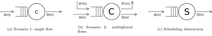
1. A Calculus with Martingale-Envelopes

(a) Scenario 1: single flow

C

A'(n) D'(n)

D(n)

(b) Scenario 2: multiplexed flows

S

A(n) D(n)

(c) Scheduling abstraction

Figure 1: Two scenarios: fg:single consists of a single flowA, whereas fg:multi has an additional cross-flowA0_{, in fg:throughs} the cross-flow from (b) is encoded in the dynamic service processS.

We consider two queueing scenarios as depicted in Figure 1, in adiscrete-time model. In the first scenario (Figure 1) a single flow A arrives at a server with capacity c > 0, whereas in the second (Figure 1), two flowsA(through-flow) andA0 (cross-flow) compete for a shared server with total capacityC=c+c0.

The cumulative arrivals are given by stochastic processes

A(m, n) = n

X

k=m+1

ak , A0(m, n) = n

X

k=m+1

a0_k , (5)

where (an)_nand (a0n)nare the instantaneous arrival processes which are throughout assumed to be stationary. As a consequence of Kolmogorov’s extension theorem, both processes (an)_n∈Nand (a0n)n∈Ncan be extended

to stationary processes (an)_n∈Z and (a0n)n∈Zhaving the same finite dimensional distributions.

In the second scenario, there exists a variety ofscheduling policies determining the priority of the data from flowAandA0, respectively. In this paper we will considerstatic priority(SP),first in, first out(FIFO), andearliest deadline first (EDF).

The network calculus approach to address scheduling queueing systems is to transform the system from Figure 1 into the system from Figure 1. The transformation occurs by encoding information about the capacity, the cross-flow, and the scheduling into a singleservice process S(m, n) which satisfies

D(n)≥(A∗S) (n) := inf

0≤k≤n{A(0, k) +S(k, n)} , (6)

forany arrival flow A(n). In some sense, the service processS(m, n) is intimately related to the impulse-response of a linear and time invariant (LTI) system (for a discussion of this analogy see, e.g., [17, 18, 14]). The performance metrics we are interested in are 1) the stationaryqueue size Q, i.e., the amount of data in the system at timen, and 2) thevirtual delay

W(n) := inf{k∈N|A(n−k)≤D(n)} ,

i.e., the time a data unit would have stayed in the system had it departed at time n. By the stationarity assumption,Qhas the following representation (see [16])

Q:=D sup n∈N

{Ar(0, n)−Cn} , (7)

whereAr _{stands for thereversed process, i.e.,}

Ar(m, n) := n

X

k=m+1

a−k ,

(where by conventionAr_{(0,0) := 0) and =}

D denotes equality in distribution.

Notation 1. Denote by−a→n the p-dimensional vector

−→

an:= (an, an+an−1, . . . , an+· · ·+an−p+1) =

Xi

k=1an−k+1

1≤i≤p

.

Notation 2. For functions h1, . . . , hp letΠhdenote the product

Πh(x1, . . . , xp) := p

Y

i=1

hi(xi).

For brevity, we omit the parameter p in Notation 2, because its value is clear from the context. We remark that we will considerp= 1 for the class of Markovian arrivals (see Section 2.2), and any values ofp

for the class ofp-order auto-regressive processes (see Section 2.3).

Definition 3 (Martingale-Envelope). For p≥0 and monotonically increasing functions h1, . . . , hp :

R+ → R+, and θ >0, we say the flow A admits a (Πh, θ, c)-martingale-envelope if for every m≥ 0 the

process

Πh(−a→n)eθ(A

r_{(m,n)−(n−m)c)}

≤Mm(n) (8)

is almost surely bounded by a supermartingaleMm.

An intuition for this definition is the following: In order to keep a queueing system in a stable regime, by Loynes’ condition, the average arrival rate has to be strictly less than the service rate. If one ignores the positivity constraint on the buffer, its expected increment (drift) is negative and thus the buffer content ‘resembles’ a supermartingale. The conceptual reason for the exponential transform is that its shape directly determines the decay rate of queueing metrics (which for Markovian arrivals are exponential). From a technical point of view, the (convex) exponential transform assigns more weight to larger arrivals, reducing the negative drift and consequently the gap between the constructed supermartingale and a martingale. Moreover, since Doob’s inequality does not differentiate between a supermartingale and a martingale, one looks to minimize the previous gap by maximizing the decay factor θ, which eventually determines the decay rate of the queueing metrics. Finally, the function h compensates for potential correlations among the increments; in particular, for i.i.d. increments,his a constant.

The monotonicity of thehi is a technical condition needed for the following important Lemma:1

Lemma 4. Forσ >0, let

N := inf{n≥0|Ar(0, n)−cn≥σ} (9)

denote the first point in time where the supremum in Eq. (7) is attained. Then for anyk≥1,

k−1

X

i=0

aN−i≥kc .

For the special case when k= 1, the inequality in Lemma 4 can be slightly strengthened to AN ≥ τ, whereτ is defined by

τ := inf{x > c|P(an ∈[x,∞))>0} ,

i.e., the smallest possible instantaneous arrival such that the buffer content increases. Note that this is only of importance if discrete distributions are considered. For continuous distributions τ is simply equal to c, and the statement is contained in Lemma 4.

The next theorems and corollaries are the central results, describing how martingale-envelopes can be used to derive bounds on the performance metricsQandW. We start with the first scenario from Figure 1, i.e., considering the case of a single flow:

Theorem 5 (_{Single Flow Bound)}. If the flow A admits a (h, θ, c)-martingale-envelope, then we have the following upper bound on the backlog and the virtual delay respectively:

P(Q≥σ)≤ E

[Πh(−a→n)] Πh(c,2c, . . . , pc)e

−θσ _,

P(W(n)≥k)≤ E

[Πh(−a→n)] Πh(c,2c, . . . , pc)e

−θck _.

Consider now the second scenario from Figure 1: two single flowsA andA0 with allocated capacities c

andc0, respectively, are multiplexed into one queueing system with a shared total capacity of C =c+c0. The resulting system can be analyzed in two different ways: Firstly, for the aggregate system both metrics

QandW can be estimated (aggregate analysis), and secondly, the virtual delayW for a single flow in the multiplexed system can be analyzed for several scheduling policies (per-flow analysis).

For both tasks, a technical definition is required:

Definition 6. For two monotonically increasing functionsh, h0 :R+→R+, define the(min,×)-convolution

by

(h⊗h0)(t) := inf

0≤s≤th(s)h

0_(t−s),

for allt∈R+. As above, if handh0 are families of functions,Π (h⊗h0)is defined componentwise:

Πh⊗h0=Y ihi⊗h

0 i .

It is easy to check thath1⊗h2 is monotonically increasing as well, and that, by definition, for alla, b:

h⊗h0(a+b)≤h(a)h0(b). (10)

1.1. Aggregate Analysis

The next theorem addresses theaggregate analysisfor the queueing system with aggregate arrivalsA+A0:

Theorem 7(_{Aggregate Envelope)}. Assume two independent arrivalsAandA0described by martingale-envelopes with parameters(Πh, θ, c)and (Πh0, θ, c0), respectively. Then the aggregate flowA+A0 admits a (Πh⊗h0, θ, C)-martingale-envelope, whereC:=c+c0.

The advantage of this theorem is that an aggregate flow can be handled in the same way as a single flow, e.g., for the constructed martingale-envelope, Theorem 5 can be evoked to derive the bounds on the backlog

Qand the virtual delayW.

Note that in Theorem 7 the flows are required to behomogeneous in the sense that they admit the same

θ in their respective envelopes. If this is not the case, the following transform of martingale-envelopes can be used:

Lemma 8. If A admits a (Πh, θ, c)-martingale-envelope and θ0 _{< θ, then A admits a Πh}θ0 θ, θ0, c

-martingale-envelope as well.

1.2. Per-Flow Analysis

We now turn to the per-flow analysis of flow A in the multiplexed queueing system equipped with a scheduling policy (Figure 1). The key element is the following technical lemma:

Lemma 9. Assume the same situation as in Theorem 7. Then for every l ≥0 and σ > 0 the following bound on the sample path holds:

P

sup n≥l

{Ar(l, n) +A0r(0, n)−Cn} ≥σ

≤ E[Πh( −→

an)]E[Πh(

−→

a0_n)] Πh⊗h0_{(c,2c, . . . , pc)}e

The crucial parameter in Lemma 9 is the parameterl, indicating how many points in time the processA

is delayed. This parameter can be adjusted according to the scheduling policy under consideration, or more precisely to the expression of the service processS depicted in Figure 1. We will next apply Lemma 9 and properly tune the parameterl for SP, FIFO, and EDF scheduling.

Let us first describe a common step. Let D denote the departure process of flowA. For every policy, for which a service processS was constructed, the bounding procedure starts with a computation similar to the one of the virtual delay in Theorem 5:

P(W(n)≥k) =P(A(0, n−k)≥D(n))≤P(A(0, n−k)≥A∗S(n))

=P

sup

0≤m≤n

{A(m, n−k)−S(m, n)} ≥0

≤P

sup n≥k

{Ar(k, n)−Sr(0, n)} ≥0

, (11)

where we again used the monotonicity ofAand the reversed representation.

Static Priority (SP). This scheduling policy always gives priority to the cross-flowA0. The service process

S(m, n) is given by (see [19]):

S(m, n) = [C(n−m)−A0(m, n)]+ , (12)

where [x]+= max{0, x}.

Corollary 10(_{SP Per-Flow Bound)}. Consider the situation as in Theorem 7, with SP as the scheduling policy. Then for the virtual delayW(n)holds:

P(W(n)≥k)≤ E[Πh(

−→

an)]E[Πh(

−→

a0_n)] Πh⊗h0_{(c,2c, . . . , pc)}e

−θck _.

First In, First Out (FIFO). For FIFO the service processS(m, n) is given by (see [20]):

S(m, n) = [C(n−m)−A0(m, n−x)]+1{n−m>x}, (13)

wherex≥0 is a parameter freely chosen, but fixed.

Corollary 11 (_{FIFO Per-Flow Bound)}. Consider the situation as in Theorem 7, with FIFO as the scheduling policy. Then for the virtual delayW(n) holds:

P(W(n)≥k)≤ E

[Πh(−a→n)]E[Πh(

−→

a0_n)] Πh⊗h0_{(c,2c, . . . , pc)}e

−θCk _.

Note the difference in the decay rate: Whereas for SP it is the per-flow capacityc, for FIFO we have the total capacityC=c+c0.

Earliest Deadline First (EDF). Now consider the case of EDF scheduling. Letdandd0 _{denote the relative} deadlines for the data units of flows A and A0, respectively. The service process S(m, n) is given by (see [21]):

S(m, n) = [C(n−m)−A0(m, n−x+ min{x, y})]+1{n−m>x} , (14)

wherex≥0 is again a free parameter, andy:=d−d0denotes the difference between the respective deadlines. It is convenient to distinguish between the casesy≥0 andy <0.

Let us first consider the case y≥0:

Corollary 12 (EDF Per-Flow Bound, y ≥0). Assume EDF is used as scheduling policy, y ≥0, and consider the situation as in Theorem 7. Then for the virtual delayW(n)holds:

P(W(n)≥k)≤ E[Πh(

−→

an)]E[Πh(

−→

a0_n)] Πh⊗h0_{(c,2c, . . . , pc)}e

Consider now the casey=d−d0<0. This is more difficult as now min{k, y}=y <0, so that for

n0∈B:={n≥k|n < k−y} ,

the argumentn0−k+ min{k, y}is negative as well. By definition (again from [21]), for those n0∈B:

A0r(n0−k+ min{k, y}) = 0 . (15)

Corollary 13 (EDF Per-Flow Bound, y < 0). Assuming EDF scheduling with y <0, for the virtual delayW(n)holds:

P(W(n)≥k)≤ E[Πh(

−→

an)]E[Πh(

−→

a0n)] Πh⊗h0_{(c,2c, . . . , pc)}e

−θ(Ck+c0y_{) +} E[Πh(−a→n)] Πh(c,2c, . . . , pc)e

−_θCk˜

,

whereθ˜is the parameter to which the flow Aadmits a (Πh,θ, C˜ )-martingale-envelope. Note that asC > c, such aθ˜exists and is greater thanθ.

2. Applications

In this section we demonstrate the versatility of the proposed martingale-envelope calculus to address several broad classes of arrival processes: with independent increments, with Markovian increments, and

p-order autoregressive.

2.1. Processes with Independent Increments

One of the simplest traffic model is given by a process with independent increments. Although not realistic, it is included here because it provides a good intuition on how the martingale-envelope calculus works. Let a1, a2. . . denote nonnegative i.i.d. random variables. The arrival process is thus A(m, n) =

Pn

k=m+1ak. Let the capacityc >0 satisfy the two stability conditions

E[a1]< c <supa1, (16)

to avoid the trivial scenarios of no queueing at all and infinite queue size, respectively.

Lemma 14. In the situation above there is aθ0>0 such thatA admits a (1, θ0, c)-martingale-envelope.

Combining the martingale-envelope from Lemma 14 with the general theory from Section 1 the following bounds hold:

Corollary 15. Consider an i.i.d. arrival flow(an)n, and a capacitycsuch that the condition from Eq. (16) holds. Then for this single flow:

P(Q≥σ)≤e−θ0c , and P(W(n)≥k)≤e−θ0ck .

With an additional i.i.d. cross-flow(a0_n)_n and capacityc0 (satisfying the corresponding stability conditions), for flowA holds in the multiplexed queueing system under scheduling:

FIFO: P(W(n)≥k)≤e−θCk SP: P(W(n)≥k)≤e−θck

EDF1: P(W(n)≥k)≤e−θ(Ck−c

0_min{k,y})

EDF2: P(W(n)≥k)≤e−θ(Ck+c

0_y

) +eθc˜0k ,

whereθ00 is the parameter in the martingale-envelope forA0,θ= min{θ0, θ00},y=d−d0,C=c+c0, andθ˜

● ●

● ●

● ● ●

● ● ● ● ● ● ● ● ● ● ●●● SP

Delay

Prob

.

Boole Martingale Simulations

0 5 10 15 20 25

1e−08

1e−05

0.01

1

100

● ●

● ●

● ● ●

● ● ● ● ● ● ● ● ● ● ●●●

● ● ● ● ● ● ● ● ● ● ● ● ●

● ●

● ● ● ● ● ● ● ● ● ●

EDF

Delay

Prob

.

Boole Martingale Simulations

0 5 10 15 20 25

1e−08

1e−05

0.01

1

100

● ● ● ● ● ● ● ● ● ● ● ● ●

● ●

● ● ● ● ● ● ● ● ● ●

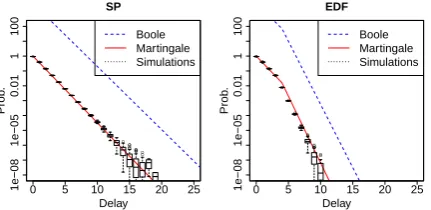
Figure 2: CCDF of the packet delay of 10 + 10 exponentially distributed subflows withλ= 1, utilizationρ= 0.95, and, for EDF,y=d−d0= 4.

EDF1 and EDF2 correspond to the casesy ≥0 andy <0, respectively (see Corollaries 12 – 13). Note that the aggregate analysis of the whole system (as in Subsection 1.1) is contained in the first part of Lemma 15, as the resulting aggregate flow (an+a0n)n is still i.i.d.

In Figure 2 simulations of the MMOO and the corresponding bounds for SP and EDF are displayed2_.

The Martingale bounds (from Corollary 15) almost match the simulations, whereas the bounds computed with Boole’s inequality are off by several orders of magnitude. As a side remark, all comparisons between bounds on virtual delays and packet delays account for the underlying Palm change of measure; moreover, we restrict to SP and the first EDF scenario; FIFO is a particular case of EDF.

2.2. Processes with Markovian Increments

The previous independence assumption on the increments is now replaced by a Markovian correlation structure, i.e., the processanis a Markov chain with state spaceS ={si|1≤i≤m}. To ensure stationarity, we assumean to be in steady state.

Letπdenote the stationary distribution andT the transition matrix of the reversed process, i.e.,

π(i) =P(an =si) and T(i, j) =P(an−1=sj|an=si).

In many cases the Markov chain isreversible and the matrix T coincides with the transition matrix of an itself. Now, for anyθ≥0, let Tθ denote theexponentially transformed transition matrix, i.e.,

Tθ(i, j) =T(i, j)eθsj .

Clearly,T =T0. Further, let λ(θ) denote the spectral radius ofTθ andv a corresponding eigenvector. The functionλ(θ) plays a similar role as the moment generating functionϕ1 in Section 2.1. It can be shown (see

[22]) thatv can be chosen to be positive and that

λ(θ) = lim n→∞E[e

θA(n)_]1

n ,

so especiallyλ(θ)≥1. Further, if the usual stability conditionE[an]< cholds,

d dθλ(θ)

_θ=0

= lim n→∞

1

nE[An] =E[an]< c= d dθe

θc

_θ=0

,

(a more rigorous proof can be found in [4]). This means that by a similar argument as in the proof of Lemma 14,θ can be chosen such that

λ(θ) =eθc . (17)

The following martingale construction can be found in [4]:

2_{For this figure (and the figures below), 100 independent simulations were run, each consisting of 10}9 _{packets. To ensure a}

Lemma 16. In the situation above (i.e., such that Eq. (17) holds), if the function hdefined byh(si) =v(i) is monotonically increasing, then the flowAadmits a (h, θ, c)-martingale-envelope.

The martingale-envelope constructed in Lemma 16 can be easily extended to Markov chains with con-tinuous state space (see again [4]).

As an application of Lemma 16 consider the arrival model as a Markov Modulated On-Off Process (MMOO), i.e., a Markov chainan jumping between the two statesOn andOff with probabilitiesαandβ, respectively. While in stateOn it transmitsR data units per time unit, and while in stateOff it does not transmit any data. The stationary distribution is given by:

π0:=P(an= 0) =

β

α+β, π1:=P(an=R) = α α+β ,

and that the process is reversible, i.e.,A=Ar. Further, in [23] it was shown that the eigenfunctionh(as defined in Lemma 16) is monotonically increasing if and only if:

Cov[an, an+1]>0⇔α <1−β . (18)

As an immediate consequence of Theorem 5 we now have:

Corollary 17. For the MMOO arrival model above and a (per-flow) capacitycsatisfyingc > Rπ1=E[an], it holds for the backlogQand the virtual delayW(n):

P(Q≥σ)≤κe−θσ , and P(W(n)≥k)≤κe−θkC ,

whereκ:=α+βh_α(0)_+β/h(R). Moreover, κ <1.

We now consider the case ofN such queueing systems (Ai, c) being multiplexed. Instead of writing down the transition matrix for the resulting process, we simply can apply Theorem 7 and Lemmas 10 – 13 to obtain bounds on the aggregate and per-flow analysis, respectively:

Corollary 18. Let

κ= (π0v0+π1v1) N

v₀N−dCR−1ev₁dCR−1e .

Then in the multiplexed queueing system with total capacityC=N c, it holds for the aggregate flow:

P(Q≥σ)≤κe−θσ , and P(W(n)≥k)≤κe−θCk ,

and for a single flow comprisingN1< N subflows under scheduling:

FIFO: P(W(n)≥k)≤κe−θCk SP: P(W(n)≥k)≤κe−θN1ck

EDF1: _P(W(n)≥k)≤κe−θ(Ck−(N−N1)cmin{k,y}) _EDF2:

P(W(n)≥k)≤κe−θ(Ck+(N−N1)cy)

+ ˜κe−θN ck˜ ,

wherey :=d−d0, and EDF1 and EDF2 correspond to y ≥0 and y <0, respectively. For EDF2,κ˜ and θ˜

denote the corresponding parameters in the queueing system which has the total capacityC =N cbut only the N1 subflows as arrivals.

It can be shown that the leading constant is exponential in N (see [23]) and thus the fundamental property from Eq. (2) is captured. As a side remark, the corresponding leading constant from [16], p. 340, is greater than one.

We point out that while the bounds in Corollary 18 for theaggregate flow have already been obtained in [23], theper-flow bounds (i.e., for SP, FIFO, and EDF) represent the contribution of this paper.

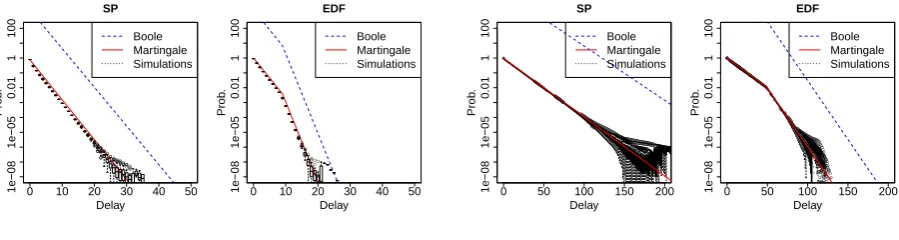
In Figure 3 simulations of the MMOO and the corresponding bounds for SP and EDF are displayed for different link utilizations. As in the case of independent increments, the Martingale bounds (from Corollary 18) are tight even at high utilizations (i.e.,ρ= 0.95), whereas the bounds calculated with Boole’s inequality (see Eq. (3)) are off by several orders of magnitude.

● ● ● ● ● ● ● ● ● ● ● ● ● ● ● ● ●● ● ● ● ● ● ● ● ● ● ● ● ● ● ● ● ●●●●●●●●●●●●● ● ● ● ● ● ● ● ● ● ● ● ● ● ● ●●●● ●●●● SP Delay Prob . Boole Martingale Simulations

0 10 20 30 40 50

1e−08 1e−05 0.01 1 100 ● ● ● ● ● ● ● ● ● ● ● ● ● ● ● ● ●● ● ● ● ● ● ● ● ● ● ● ● ● ● ● ● ●●●●●●●●●●●●● ● ● ● ● ● ● ● ● ● ● ● ● ● ● ●●●● ●●●● ● ● ● ● ● ● ● ● ●● ●● EDF Delay Prob . Boole Martingale Simulations

0 10 20 30 40 50

1e−08 1e−05 0.01 1 100 ● ● ● ● ● ● ● ● ●● ●●

(a) Utilizationρ= 0.75, andd−d0= 9.

● ● ●●●●●●●●●●● ● ● ●●●●●●●●●●●●●●●●●●●●●●●●●● ● ●●●●●●●● ● ●●●●● ● ● ● ● ● ● ● ● ●●●●●●●●●●●●●●●●●●●●●●●●●●●●●●●●●●●●●●●●●●●●●●●●●●●●●●●●●●●●●●●●●●●●●●●●●●●●●●●●●●●●●●●●●●●●●●●●●●●●●● ● ● ● ● ● ● ●● ● ● ● ● ●● ● ● ● ● ● ● ● ● ● ● ●● ● ● ● ● ● ● ● ● ● ●● ● ● ● ●● ● ● ● ● ● ● ● ● ●● ● ● ● ● ● ● ● ● ●● ● ● ● ●● ● ● ● ● ● ● ●● ● ● ● ●●●●●●●●●●●●● SP Delay Prob . Boole Martingale Simulations

0 50 100 150 200

1e−08 1e−05 0.01 1 100 ● ● ●●●●●●●●●●● ● ● ●●●●●●●●●●●●●●●●●●●●●●●●●● ● ●●●●●●●● ● ●●●●● ● ● ● ● ● ● ● ● ●●●●●●●●●●●●●●●●●●●●●●●●●●●●●●●●●●●●●●●●●●●●●●●●●●●●●●●●●●●●●●●●●●●●●●●●●●●●●●●●●●●●●●●●●●●●●●●●●●●●●● ● ● ● ● ● ● ●● ● ● ● ● ●● ● ● ● ● ● ● ● ● ● ● ●● ● ● ● ● ● ● ● ● ● ●● ● ● ● ●● ● ● ● ● ● ● ● ● ●● ● ● ● ● ● ● ● ● ●● ● ● ● ●● ● ● ● ● ● ● ●● ● ● ● ●●●●●●●●●●●●● ● ● ●●●●●●●●●●●●●●●●●●●●●●●●●●●●●●●●●●●●●●●●●●●●●●●●●●●●●●●●●●●●●●●●●●●●●●●●●●●●●●●●●●●●●● ●●● ● ●● ●●●●●●●●● ●●●●●●●●●●●●●●●●●●●●●●●●●●●● ● ● ● ● ● ● ● ● ●●●●● ● ● ● ● ● ● ● ● ● ● ●●●●●● ● ● ●●● ● ● ● ● ● ● ● ● ● ● ● ● ● ● ● ● ● ● ● ● ● ● ● ● ● ● ● ● ● ● ● ● ● ● ● ● ● ● ● ● ● ● ● ● ● ● ● ● ● ● ● ● ● ● ● ● ● ● ● ● ● ● ● ● ● ● ● ● ● ● ● ● ● ● ● ● ● ● ● ● ● ● ● ● ● ● ● ● ● ● ● ● ● ● ● ● ● ● ● ● ● ● ● ● ● ● ● ● ● ● ● ● ● ● ● ● ● ● ● ● ● ● ● ● ● ● ● ● ● ● ● ● ● ● ● ● ● ● ● ● ● ● ● ● ● ● ● ● ● ● ● ● ● ● ● ● ● ● ● ● ● ● ● ● ● ● ● ● ● ● ● ● ● ● ● ● ● ● ● ● ● ● ● ● ● ● ● ● ● ● ● ● ● ● ● ● ● ● ● ● ● ● ● ● ● ● ● ● ● ● ● ● ● ● ● ● ● ● ● ● ● ● ● ● ● ● ● ● ● ● ● ● ● ● ● ● ● ● ● ● ● ● ● ● ● ● ● ● ● ● ● ● ● ● ● ● ● ● ● ● ● ● ● ● ● ● ● ● ● ● ● ● ● ● ● ● ● ● ● ● ● ● ● ● ● ● ● ● ● ● ● ● ● ● ● ● ● ● ● ● ● ● ● ● ● ● ● ● ● ● ● ● ● ● ● ● ● ● ● ● ● ● ● ● ● ● ● ● ● ● ● ● ● ● ● ● ● ● ● ● ● ● ● ● ● ● ● ● ● ● ● ● ● ● ● ● ● ● ● ● ● ● ● ● ● ● ● ● ● ● ● ● ● ● ● ● ● ● ● ● EDF Delay Prob . Boole Martingale Simulations

0 50 100 150 200

1e−08 1e−05 0.01 1 100 ● ● ●●●●●●●●●●●●●●●●●●●●●●●●●●●●●●●●●●●●●●●●●●●●●●●●●●●●●●●●●●●●●●●●●●●●●●●●●●●●●●●●●●●●●● ●●● ● ●● ●●●●●●●●● ●●●●●●●●●●●●●●●●●●●●●●●●●●●● ● ● ● ● ● ● ● ● ●●●●● ● ● ● ● ● ● ● ● ● ● ●●●●●● ● ● ●●● ● ● ● ● ● ● ● ● ● ● ● ● ● ● ● ● ● ● ● ● ● ● ● ● ● ● ● ● ● ● ● ● ● ● ● ● ● ● ● ● ● ● ● ● ● ● ● ● ● ● ● ● ● ● ● ● ● ● ● ● ● ● ● ● ● ● ● ● ● ● ● ● ● ● ● ● ● ● ● ● ● ● ● ● ● ● ● ● ● ● ● ● ● ● ● ● ● ● ● ● ● ● ● ● ● ● ● ● ● ● ● ● ● ● ● ● ● ● ● ● ● ● ● ● ● ● ● ● ● ● ● ● ● ● ● ● ● ● ● ● ● ● ● ● ● ● ● ● ● ● ● ● ● ● ● ● ● ● ● ● ● ● ● ● ● ● ● ● ● ● ● ● ● ● ● ● ● ● ● ● ● ● ● ● ● ● ● ● ● ● ● ● ● ● ● ● ● ● ● ● ● ● ● ● ● ● ● ● ● ● ● ● ● ● ● ● ● ● ● ● ● ● ● ● ● ● ● ● ● ● ● ● ● ● ● ● ● ● ● ● ● ● ● ● ● ● ● ● ● ● ● ● ● ● ● ● ● ● ● ● ● ● ● ● ● ● ● ● ● ● ● ● ● ● ● ● ● ● ● ● ● ● ● ● ● ● ● ● ● ● ● ● ● ● ● ● ● ● ● ● ● ● ● ● ● ● ● ● ● ● ● ● ● ● ● ● ● ● ● ● ● ● ● ● ● ● ● ● ● ● ● ● ● ● ● ● ● ● ● ● ● ● ● ● ● ● ● ● ● ● ● ● ● ● ● ● ● ● ● ● ● ● ● ● ● ● ● ● ● ● ● ● ● ● ● ● ● ● ● ●

(b) Utilizationρ= 0.95, andd−d0= 49.

Figure 3: CCDF of the packet delay withN1=1₂N= 10,α= 0.1,β= 0.5, andR= 1.

2.3. Autoregressive Arrival Models

As a third example we consider autoregressive processes. Roughly, a p-order autoregressive process (AR(p)) evolves by rescaling the p previous values of the process and adding Gaussian white noise, i.e., uncorrelated Gaussian random variables. Although implicitly contained in the theory of (p-order) Markov processes, the different representation has the advantage of providing closed form solutions to the perfor-mance metrics.

We start with the formal definition ofAR(p). For simplicity, we assume throughout that the white noise is not only uncorrelated but independent.

Definition 19. Let p≥1, Z0, Z1, Z2,· · · ∼ N0,1 i.i.d., ϕ1, . . . , ϕp ∈[0,1), ϕ=P p

k=1ϕk, and µ, σ >0. If the relation

an= p

X

k=1

ϕkan−k+ (1−ϕ)µ+ (1−ϕ)σZn (19)

holds, the process(an)n is called thep-order autoregressive process,AR(p).

It can be shown (see, e.g., [15], p. 85) that if all the (complex) roots of thecharacteristic polynomial

χ(z) = 1− p

X

k=1

ϕkzk

lie outside the unit interval, i.e., χ(z) = 0 ⇒ |z| > 1, then the process AR(p) is stationary. We assume throughout that this is fulfilled. As above, we apply Kolmogorov’s theorem to obtain an extended process (an)_n∈Z which is still stationary and satisfying Eq. (19). Moreover, asAR(p) is clearly a Gaussian process itself, it is also reversible (see [24]), i.e.,Ar_=A.

Note that althoughE[an] =µfor alln∈Z, by the correlation ofAR(p) the variance V[an] is not equal toσ, but must be derived using the Yule-Walker-Equations (see again [15], p. 239).

As in the previous examples we interpretan as the instantaneous arrival at timen, i.e.,

An := n

X

k=1

ak

Theorem 20. Let θ= 2c−µ_σ2 and for1≤k≤p

hi(t) :=e

θ

1−ϕϕkt _.

Then the flowA admits a(Πh, θ, c)-martingale-envelope.

Note that for p= 0 we recover the case of independent increments as in Subsection 2.1.

Clearly, the product function Πh is monotonically increasing in its parameters Pk

i=1ti

0≤k≤p. So

Lemma 4 can be applied to obtain

Πh(−a→N)≥Πh(c, . . . , pc) =e

θ

1−ϕc

Pp

k=1kϕk _{, (20)}

whereN denotes the stopping time from Eq. (9). Let now

Y := p

X

k=1

ϕk k

X

i=1

an−i+1

(note that in distribution this is independent ofn). Y is normally distributed with_E[Y] =µPp

k=1kϕk. Let

ν2_:=

V[Y] denote its variance, which again can be calculated using the Yule-Walker-Equations.

Considering the single flow scenario from Figure 1 and Theorem 5, the following bounds hold:

Corollary 21. For the autoregressive arrival modelAR(p)with a capacity c satisfyingc > µ, let

κ=e θ(µ−c)

1−ϕ

_Pp

k=1kϕk− ν

2 (1−ϕ)σ2

, and θ= 2c−µ

σ2 .

Then for the backlogQand virtual delayW(n)hold

P(Q≥σ)≤κe−θσ , and P(W(n)≥k)≤κe−θck .

Let us consider the case ofp= 1, i.e.,:

an=ϕan−1+ (1−ϕ)µ+ (1−ϕ)σZn .

This special case allows an explicit calculation of the varianceν2_:

ν2=V[ϕan] =V[ϕan+1] =ϕ2V[ϕan+σ(1−ϕ)Zn+1] =ϕ2

ν2+σ2(1−ϕ)2 ,

and thusν2_=σ2 (1−ϕ)ϕ2

1+ϕ . The leading constantκfrom Corollary 21 reduces to

κ=E[h(an)]

h(c) =e

θ(µ−c) 1−ϕ

ϕ− ν2

(1−ϕ)σ2

=e

θ(µ−c) 1−ϕ

ϕ−₁₊ϕ2_ϕ =e

θϕ(µ−c)

1−ϕ2 . (21)

Note that in this caseκ∈(0,1]. Therefore, with regards to the queue sizeQ, the following bound holds:

P(Q > σ)≤e

θϕ(µ−c) 1−ϕ2 _e−θσ _.

This bound improves the known results drastically: e.g., in [16], p. 340, an additional factor occurs, which depends on an upper bound on the increment process. As theGaussian white noise is unbounded, the corresponding bound from [16] is meaningless.

● ● ●●●● ● ● ●●●●●●●●●●●●●●●●●●●●●●●●●●●●●●●●●●●●●●●●●●●●●●●●●●●●●●●● ● ● ●●●●●●● ●● ● ●●●●●●●●●●●●●●●●●●●●●●●●●●●●●●●●●●●●●●●●●●●●●●●●●●●●●●●●●●●●●●●●●●●●●●●●●●●●●●●●●●●●●●●●●●●● ● ● ● ● ● ● ● ● ● ● ● ● ● ●●● ● ● ●●●●●●●●●●●●● SP Delay Prob . Martingale Simulations

0 25 50 75

1e−08

1e−04

1 ●● ●●●● ● ● ●●●●●●●●●●●●●●●●●●●●●●●●●●●●●●●●●●●●●●●●●●●●●●●●●●●●●●●● ● ● ●●●●●●● ●● ● ●●●●●●●●●●●●●●●●●●●●●●●●●●●●●●●●●●●●●●●●●●●●●●●●●●●●●●●●●●●●●●●●●●●●●●●●●●●●●●●●●●●●●●●●●●●● ● ● ● ● ● ● ● ● ● ● ● ● ● ●●● ● ● ●●●●●●●●●●●●● ● ● ● ● ● ●●●●●●●●●●●●●●●●●●●●●●●●●●●●●●●●●●● ●●●●●●●●●●●●●●●● ● ●●● ● ● ● ● ●●●●●●●●●●●●●●●●●●●●●●●●●●●●●●●● ● ● ●●●●●● ● ● ● ● ● ●● ● ●●● ●● EDF Delay Prob . Martingale Simulations

0 25 50 75

1e−08

1e−04

1 ●● ● ● ● ●●●●●●●●●●●●●●●●●●●●●●●●●●●●●●●●●●● ●●●●●●●●●●●●●●●● ● ●●● ● ● ● ● ●●●●●●●●●●●●●●●●●●●●●●●●●●●●●●●● ● ● ●●●●●● ● ● ● ● ● ●● ● ●●● ●●

(a)AR(1),ϕ1= 0.6

●● ● ●●●●●●●●●●●●●● ●●●●●●● ● ● ●●●●●●●●●●●●● ●●●●●●●●●● ● ● ● ● ● ● ● ● ● ● ● ● ● ● ●●●●●●●●●● ●●●●●_{●●●●●●} ● ●●●●●●●●●●●● ● ● SP Delay Prob . Martingale Simulations

0 25 50 75

1e−08 1e−04 1 ●● ● ●●●●●●●●●●●●●● ●●●●●●● ● ● ●●●●●●●●●●●●● ●●●●●●●●●● ● ● ● ● ● ● ● ● ● ● ● ● ● ● ●●●●●●●●●● ●●●●●_{●●●●●●} ● ●●●●●●●●●●●● ● ● ● ●● ●●●● ● ● ●●●●●●●●●●●●●●●●●●●●●●● ● ● ● ●●● ● ● ● ● ● ● ● ● ● ● ●●●● ● ● ●●●●●●●● ● ●● ● ●●●●● ● ●● ● ● ●● EDF Delay Prob . Martingale Simulations

0 25 50 75

1e−08 1e−04 1 ● ●● ●●●● ● ● ●●●●●●●●●●●●●●●●●●●●●●● ● ● ● ●●● ● ● ● ● ● ● ● ● ● ● ●●●● ● ● ●●●●●●●● ● ●● ● ●●●●● ● ●● ● ● ●●

(b)AR(2),ϕ1= 0.4,ϕ2= 0.2

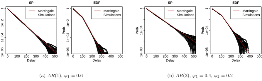
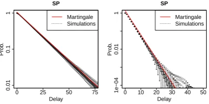
Figure 4: CCDF of the packet delay forAR(1) (fg:ar1) andAR(2) (fg:ar2), with parametersµ= 0.5,σ= 1, utilizationρ= 0.75, and, for EDF,y=d−d0= 24.

● ●●●●●●●●●●●●●●●●●●●●●●●●●●●●●●●●●●●●●●●●●●●●●●●●●●●●●●●●●●●●●●●●●●●●●●●●●●●●●●●●●●●●●●●●●●●●●●●●●●●●●●●●●●●●●●●●●●●●●●●●●●●●●●●●●●●●●●●●●●●●●●●●●●●●●●●●●●●●●●●●●●●●●●●●●●●●●●●●●●●●●●●●●●●●●●●●●●●●●●●●●●●●●●●●●●●●●●●●●●●●●●●●●●●●●●●●●●●●●●●●●●●●●●●●●●●●●●●●●●●●●●●●●●●●●●●●●●●●●●●●●●●●●●●●●●●●●●●●●●●●●●●●●●●●●●●●●●●●●●●●●●●●●●●● ● ● ● ●●●●●●●●●●●●●●●●●●●● ● ● ● ● ●●●●●●●●●●●●●●●●●●●●●● ● ● ● ● ● ● ● ● ● ● ● ● ● ● ● ● ● ●●●● ● ● ● ● ● ● ● ● ● ●● ● ● ● ● ● ● ● ● ● ● ● ● ● ● ●● ● ● ● ● ● ● ● ● ● ● ● ● ● ● ● ● ● ● ●● ● ● ● ● ● ● ● ● ● ● ● ● ● ● ● ● ● ● ●● ● ● ● ● ● ● ● ● ● ● ● ● ● ● ● ● ● ● ● ● ● ● ● ● ●●●● ● ● ● ● ● ● ● ● ● ● ● ● ● ● ● ● ● ● ● ● ● ● ● ● ●●●● ● ● ● ● ● ● ● ● ● ● ● ● ● ● ● ● ● ● ● ● ● ● ● ● ● ● ● ● ● ● ● ●●●● ● ● ● ● ● ● ● ● ● ● ● ● ● ● ● ● ● ● ● ● ● ● ● ● ●●●● ● ● ● ● ● ● ● ● ● ● ● ● ● ● ● ● ● ● ● ● ● ● ● ● ●●●● ● ● ● ● ● ● ● ● ● ● ● ● ● ● ● ● ● ● ● ● ● ● ● ● ●●●● ● ● ● ● ● ● ● ● ● ● ● ● ● ● ● ● ● ● ● ● ●●●● ● ● ● ● ● ● ● ● ● ● ● ● ● ● ● ● ● ● ●●● ● ● ● ● ● ● ● ● ● ● ● ● ● ●●● ● ● ● ● ● ● ● ● ● ● ● ● ● ● ● ● ● ●●● ● ● ● ● ● ● ● ● ● ● ● ● ●●● ● ● ● ● ● ● ● ● ● ● ● ●●●●●●●●●●●●●●●●●●●●●●●●●●●●●●●●●●●●●●●●●●●●●●●●●●●●●●●●●●●●●●●●●●●●●●●●●●●●●●●●●●●●●●●●●●●●●●●●●●●●●●●●●●●●●●●●●●●●●●●●●● SP Delay Prob . Martingale Simulations

0 100 200 300 400 500

1e−06 1e−04 1e−2 1 ● ●●●●●●●●●●●●●●●●●●●●●●●●●●●●●●●●●●●●●●●●●●●●●●●●●●●●●●●●●●●●●●●●●●●●●●●●●●●●●●●●●●●●●●●●●●●●●●●●●●●●●●●●●●●●●●●●●●●●●●●●●●●●●●●●●●●●●●●●●●●●●●●●●●●●●●●●●●●●●●●●●●●●●●●●●●●●●●●●●●●●●●●●●●●●●●●●●●●●●●●●●●●●●●●●●●●●●●●●●●●●●●●●●●●●●●●●●●●●●●●●●●●●●●●●●●●●●●●●●●●●●●●●●●●●●●●●●●●●●●●●●●●●●●●●●●●●●●●●●●●●●●●●●●●●●●●●●●●●●●●●●●●●●●●● ● ● ● ●●●●●●●●●●●●●●●●●●●● ● ● ● ● ●●●●●●●●●●●●●●●●●●●●●● ● ● ● ● ● ● ● ● ● ● ● ● ● ● ● ● ● ●●●● ● ● ● ● ● ● ● ● ● ●● ● ● ● ● ● ● ● ● ● ● ● ● ● ● ●● ● ● ● ● ● ● ● ● ● ● ● ● ● ● ● ● ● ● ●● ● ● ● ● ● ● ● ● ● ● ● ● ● ● ● ● ● ● ●● ● ● ● ● ● ● ● ● ● ● ● ● ● ● ● ● ● ● ● ● ● ● ● ● ●●●● ● ● ● ● ● ● ● ● ● ● ● ● ● ● ● ● ● ● ● ● ● ● ● ● ●●●● ● ● ● ● ● ● ● ● ● ● ● ● ● ● ● ● ● ● ● ● ● ● ● ● ● ● ● ● ● ● ● ●●●● ● ● ● ● ● ● ● ● ● ● ● ● ● ● ● ● ● ● ● ● ● ● ● ● ●●●● ● ● ● ● ● ● ● ● ● ● ● ● ● ● ● ● ● ● ● ● ● ● ● ● ●●●● ● ● ● ● ● ● ● ● ● ● ● ● ● ● ● ● ● ● ● ● ● ● ● ● ●●●● ● ● ● ● ● ● ● ● ● ● ● ● ● ● ● ● ● ● ● ● ●●●● ● ● ● ● ● ● ● ● ● ● ● ● ● ● ● ● ● ● ●●● ● ● ● ● ● ● ● ● ● ● ● ● ● ●●● ● ● ● ● ● ● ● ● ● ● ● ● ● ● ● ● ● ●●● ● ● ● ● ● ● ● ● ● ● ● ● ●●● ● ● ● ● ● ● ● ● ● ● ● ●●●●●●●●●●●●●●●●●●●●●●●●●●●●●●●●●●●●●●●●●●●●●●●●●●●●●●●●●●●●●●●●●●●●●●●●●●●●●●●●●●●●●●●●●●●●●●●●●●●●●●●●●●●●●●●●●●●●●●●●●● ● ● ● ● ● ● ●●●●●●●●●●●●●●●●●●●●●●●●●●●●●●●●●●●●●●●●●●●●●●●●●●●●●●●●●●●●●●●●●●●●●●●●●●●●●●●●●●●●●●●●●●●●●●●●●●●●●●●●●●●●●●●●●●●●●●●●●●●●●●●●●●●●●●●●●●●●●●●●●●●●●●●●●●●●●●●●●●●●●●●●●●●●●●●●●●●●●●●●●●●●●●●●●●●●●●●●●●●●●●●●●●●●●●●●●●●●●●●● ● ●●● ● ● ● ●●●●●●●●●●●●●●●●●●●●●●●●●●●●●●●●●●●● ● ● ● ● ● ● ● ● ● ●●●●●●●●●● ● ● ● ● ● ● ● ● ● ● ● ● ● ● ● ●●●●● ● ● ● ● ● ● ● ● ● ● ● ● ● ● ● ● ● ● ●●●●● ● ● ● ● ● ● ● ● ● ● ● ● ● ● ● ● ●●●●● ● ● ● ● ● ● ● ● ● ● ● ● ● ● ● ●●●●●●●●●●●●●●●●●●●●●●●●●●●●●●●●●●●●●●●●●●●●●●●●●●●●●●●●●●●●●●● ● ● ● ● ● ● ● ● ● ● ● ● ● ● ● ● ● ● ● ● ● ● ● ● ● ● ● ● ● ● ● ● ● ● ● ● ● ● ● ● ● ● ● ● ● ● ● ● ● ● ● ● ● ● ● ● ● ● ● ● ● ● ● ● ● ● ● ● ● ● ● ● ●●●●●●●●●●●●●●●●●●●●●●●●●●●●●●●●●●●●●●●●●●●●●●●●●●● EDF Delay Prob . Martingale Simulations

0 100 200 300 400 500

1e−06

1e−04

1e−2

1 ●●●●●●●●●●●●●●●●●●●●●●●●●●●●●●●●●●●●●●●●●●●●●●●●●●●●●●●●●●●●●●●●●●●●●●●●●●●●●●●●●●●●●●●●●●●●●●●●●●●●●●●●●●●●●●●●●●●●●●●●●●●●●●●●●●●●●●●●●●●●●●●●●●●●●●●●●●●●●●●●●●●●●●●●●●●●●●●●●●●●●●●●●●●●●●●●●●●●●●●●●●●●●●●●●●●●●●●●●●●●●●●●●●●●●●

● ●●● ● ● ● ●●●●●●●●●●●●●●●●●●●●●●●●●●●●●●●●●●●● ● ● ● ● ● ● ● ● ● ●●●●●●●●●● ● ● ● ● ● ● ● ● ● ● ● ● ● ● ● ●●●●● ● ● ● ● ● ● ● ● ● ● ● ● ● ● ● ● ● ● ●●●●● ● ● ● ● ● ● ● ● ● ● ● ● ● ● ● ● ●●●●● ● ● ● ● ● ● ● ● ● ● ● ● ● ● ● ●●●●●●●●●●●●●●●●●●●●●●●●●●●●●●●●●●●●●●●●●●●●●●●●●●●●●●●●●●●●●●● ● ● ● ● ● ● ● ● ● ● ● ● ● ● ● ● ● ● ● ● ● ● ● ● ● ● ● ● ● ● ● ● ● ● ● ● ● ● ● ● ● ● ● ● ● ● ● ● ● ● ● ● ● ● ● ● ● ● ● ● ● ● ● ● ● ● ● ● ● ● ● ● ●●●●●●●●●●●●●●●●●●●●●●●●●●●●●●●●●●●●●●●●●●●●●●●●●●●

(a)AR(1),ϕ1= 0.6

● ● ● ●●●●●●●●●●●●●●●●●●●●●●●●●●●●●●●●●●●●●●●●●●●●●●●●●●●●●●●●●●●●●●●●●●●●●●●●●●●●●●●●●●●●●●●●●●●●●●●●●●●●●●●●●●●●●●●●●●●●●●●●●●●●●●●●●●●●●●●●●●●●●●●●●●●●●●●●●●●●●●●●●●●●●●●●●●●●●●●●●●●●●●●●●●●●●●●●●●●●●●●●●●●●●●●●●●●●●●●●●●●●●●●●●●●●●●●●●●●●●●●●●●●●●●● ● ● ●●●●●●●●●●● ● ●●●●●●●●●●●●●●●●●●●●●●●●●●●●●●●●●●●●●●●●●●●●●●●●●●●●●●●●●●●●●●●●●●●●●●●●●●●●●●●●●●●●●●●●●●●●●●●●●●●●●●●● ● ● ● ● ● ● ● ● ● ● ● ● ● ● ●●●●●●●●●●●●●●●●●●●●●●●●●●●●●●●●●●●●●●●●●●●●●●●●●●●●●●●●●●●●●●●●●●●●●●●●●●●●●●●●●●●●●●●●●●●●●●●●●●●●●●●●●●●●●●●●●●●●●●●●●●●● ●●●●● ● ● ● ● ● ● ● ● ● ● ● ● ● ● ● ● ●●●●●●●●●●●●●●●●●●●●●●●●●●●●●●●●●●●●●●●●●●●●●●●●●● ● ● ● ● ● ● ● ● ● ● ● ● ● ● ● ● ● ●●● ● ● ● ● ● ● ● ● ● ● ● ● ● ● ● ● ● ●●● ● ● ● ● ● ● ● ● ● ● ● ● ● ● ● ● ● ●●●● ● ● ● ● ● ● ● ● ● ● ● ● ● ● ● ● ● ● ● ● ● ● ● ● ● ● ● ● ● ● ● ● ● ● ● ● ●●●● ● ● ● ● ● ● ● ● ● ● ● ● ●●●● ● ● ● ● ● ● ● ● ● ● ● ● ●●●● ● ● ● ● ● ● ● ● ● ● ● ● ●●●● ● ● ● ● ● ● ● ● ● ● ● ● ● ● ● ● ●●●● ● ● ● ● ● ● ● ● ● ● ● ● ●●●● ● ● ● ● ● ● ● ● ● ● ● ● ●●●● ● ● ● ● ● ● ● ● ● ● ● ● ●●●● ● ● ● ● ● ● ● ● ● ● ● ● ●●●● ● ● ● ● ● ● ● ● ● ● ● ● ●●●● ● ● ● ● ● ● ● ● ● ● ● ● ●●●● ● ● ● ● ● ● ● ● ● ● ● ● ●●●●●●●●●●●●●●●●●●●●●●●●●●●●●●●● ● ● ● ● ●●●● ● ● ● ● ● ● ● ● ● ● ● ● ●●●● ● ● ● ● ● ● ● ● ● ● ● ● ●●●●●●●●●●●●●●●●● ● ● ● ●● ●●●●● SP Delay Prob . Martingale Simulations

0 100 200 300 400 500

1e−08

1e−04

1 ●● ● ●●●●●●●●●●●●●●●●●●●●●●●●●●●●●●●●●●●●●●●●●●●●●●●●●●●●●●●●●●●●●●●●●●●●●●●●●●●●●●●●●●●●●●●●●●●●●●●●●●●●●●●●●●●●●●●●●●●●●●●●●●●●●●●●●●●●●●●●●●●●●●●●●●●●●●●●●●●●●●●●●●●●●●●●●●●●●●●●●●●●●●●●●●●●●●●●●●●●●●●●●●●●●●●●●●●●●●●●●●●●●●●●●●●●●●●●●●●●●●●●●●●●●●● ● ● ●●●●●●●●●●● ● ●●●●●●●●●●●●●●●●●●●●●●●●●●●●●●●●●●●●●●●●●●●●●●●●●●●●●●●●●●●●●●●●●●●●●●●●●●●●●●●●●●●●●●●●●●●●●●●●●●●●●●●● ● ● ● ● ● ● ● ● ● ● ● ● ● ● ●●●●●●●●●●●●●●●●●●●●●●●●●●●●●●●●●●●●●●●●●●●●●●●●●●●●●●●●●●●●●●●●●●●●●●●●●●●●●●●●●●●●●●●●●●●●●●●●●●●●●●●●●●●●●●●●●●●●●●●●●●●● ●●●●● ● ● ● ● ● ● ● ● ● ● ● ● ● ● ● ● ●●●●●●●●●●●●●●●●●●●●●●●●●●●●●●●●●●●●●●●●●●●●●●●●●● ● ● ● ● ● ● ● ● ● ● ● ● ● ● ● ● ● ●●● ● ● ● ● ● ● ● ● ● ● ● ● ● ● ● ● ● ●●● ● ● ● ● ● ● ● ● ● ● ● ● ● ● ● ● ● ●●●● ● ● ● ● ● ● ● ● ● ● ● ● ● ● ● ● ● ● ● ● ● ● ● ● ● ● ● ● ● ● ● ● ● ● ● ● ●●●● ● ● ● ● ● ● ● ● ● ● ● ● ●●●● ● ● ● ● ● ● ● ● ● ● ● ● ●●●● ● ● ● ● ● ● ● ● ● ● ● ● ●●●● ● ● ● ● ● ● ● ● ● ● ● ● ● ● ● ● ●●●● ● ● ● ● ● ● ● ● ● ● ● ● ●●●● ● ● ● ● ● ● ● ● ● ● ● ● ●●●● ● ● ● ● ● ● ● ● ● ● ● ● ●●●● ● ● ● ● ● ● ● ● ● ● ● ● ●●●● ● ● ● ● ● ● ● ● ● ● ● ● ●●●● ● ● ● ● ● ● ● ● ● ● ● ● ●●●● ● ● ● ● ● ● ● ● ● ● ● ● ●●●●●●●●●●●●●●●●●●●●●●●●●●●●●●●● ● ● ● ● ●●●● ● ● ● ● ● ● ● ● ● ● ● ● ●●●● ● ● ● ● ● ● ● ● ● ● ● ● ●●●●●●●●●●●●●●●●● ● ● ● ●● ●●●●● ● ● ● ●●● ● ● ● ●●●●●●●●●●●●●●●●●●●●●●●●●●●● ● ● ● ●●●●●●●●●●●●●●●●●●●●●●●●●●●●●●●●●●●●●●●●●●●●●●●●●●●●●●●●●●●●●●●●●●●●●●● ● ● ● ● ● ● ● ● ●●●●●●● ● ● ● ● ● ● ● ● ● ●●●●●●●●●●●●●●●●●●●●●●●●●●●●●●●●●●●●●●●●●●●●●● ● ● ● ● ● ● ● ● ● ● ● ● ● ●● ● ● ● ● ● ● ● ● ● ● ● ● ● ● ● ● ● ● ● ● ● ● ● ● ●● ● ● ● ● ● ● ● ● ● ● ● ● ● ● ● ● ● ● ● ● ● ● ●● ● ● ● ● ● ● ● ● ● ● ● ● ● ● ● ●●●●●●●●●●●●●●●●● ● ● ● ● ● ● ● ● ● ● ● ● ●●●●●● ● ● ● ● ● ● ● ● ● ● ●●●●●●●●●●●●●●●●●●●●●●●●●●●●●●● EDF Delay Prob . Martingale Simulations

0 100 200 300 400 500

1e−08

1e−04

1 ●●●●●● ● ● ● ●●●●●●●●●●●●●●●●●●●●●●●●●●●● ● ● ● ●●●●●●●●●●●●●●●●●●●●●●●●●●●●●●●●●●●●●●●●●●●●●●●●●●●●●●●●●●●●●●●●●●●●●●● ● ● ● ● ● ● ● ● ●●●●●●● ● ● ● ● ● ● ● ● ● ●●●●●●●●●●●●●●●●●●●●●●●●●●●●●●●●●●●●●●●●●●●●●● ● ● ● ● ● ● ● ● ● ● ● ● ● ●● ● ● ● ● ● ● ● ● ● ● ● ● ● ● ● ● ● ● ● ● ● ● ● ● ●● ● ● ● ● ● ● ● ● ● ● ● ● ● ● ● ● ● ● ● ● ● ● ●● ● ● ● ● ● ● ● ● ● ● ● ● ● ● ● ●●●●●●●●●●●●●●●●● ● ● ● ● ● ● ● ● ● ● ● ● ●●●●●● ● ● ● ● ● ● ● ● ● ● ●●●●●●●●●●●●●●●●●●●●●●●●●●●●●●●

(b)AR(2),ϕ1= 0.4,ϕ2= 0.2

Figure 5: CCDF of the packet delay forAR(1) (fg:ar195)andAR(2)(f g:ar2), withparametersµ = 0.5, σ = 1, utilization

ρ= 0.95, and, for EDF,y=d−d0_{= 99.}

Corollary 22. With the definitions as in Corollary 21 for the multiplexed queueing system with aggregate capacity2cholds:

P(Q≥σ)≤κ2e−θσ , and P(W(n)≥k)≤κ2e−θ2ck ,

and for a single flow under scheduling:

FIFO: _P(W(n)≥k)≤κ2e−θ2ck SP: _P(W(n)≥k)≤κ2e−θck

EDF1: P(W(n)≥k)≤κ2e−θ(2ck−cmin{k,y}) EDF2: P(W(n)≥k)≤κ2e−θ(2ck+cy)+ ˜κe−θ˜2ck .

Again, y :=d−d0, and EDF1 and EDF2 correspond to y ≥0 and y <0, respectively;κ˜ andθ˜denote the constantsκandθ with cexchanged by 2c.

Note that as the sum of independent autoregressive processes is still autoregressive, the aggregate bounds in the first part of Corollary 22 could also be obtained by applying Corollary 21 to thesingle flowAn+A0n. As the correspondingκis independent of the number of flows, applying Eq. (A.2) iteratively leads to bounds retaining the fundamental exponential decay property from Eq. (2).

Martingale Bound Delay Probability

Delay

Prob

.

(a) Initial rate larger than asymptotic rate

Martingale Bound Delay Probability

Delay

Prob

.

(b) Initial rate smaller than asymptotic rate

Figure 6: Possible CCDF of the delay. Depending on the flows’ burstiness the martingale (exponential) bounds are inevitably loose for small or large delays.

obtain bounds, since the sum on the right hand side in Eq. (3) seems not to converge. A follow-up discussion on tightness will be given in the next section.

3. Discussion

In this section we discuss on the tightness issues of the martingale-based method and provide some insight into a contriving idiosyncracy between discrete vs. continuous-time results. We divide the discussion according to the flows’ burstiness level.

3.1. Bursty Flows

Although the bounds illustrated in Figures 2-5 are seemingly accurate, the bounds degrade with the level of correlations within the arrivals. This trend can be particularly noticed for 1-order vs. 2-order autoregressive processes (see Figure 2.3 vs. 2.3); the same could be observed by reducing the scale of the x-axis in Figures 2.3 and 2.3. One explanation is that on a logarithmicy-axis the simulations throughout are seemingly convex, i.e., the probabilities in an initial phase decay faster than asymptotically (this behavior has been in fact convincingly shown to hold for bursty flows in [3]). In contrast, as the martingale-envelope is based on an exponential transform, itcan only render bounds of the form of the (generalized) exponential distribution (i.e., P rob ≤ κe−θx_{), whence the straight lines in the plots. In other words, the longer the} “initial phase” of the true distribution is, or more generally the level of long-range correlations, the larger the gap is between the distribution and the obtained bounds. We point out that the bounds match in fact simulations at the starting point (although difficult to visually perceive from the printed plots) of the true distribution. To more conveniently contrast the true distribution and thebest possible exponential bounds, see Figure 3.1.

A possible approach to reduce this inherent gap would be to use hyperexponential rather than exponential transforms, i.e., functions of the form p1eθ1x+p2eθ2x, where the parametersp1, λ1 and p2, λ2 are scaled

accordingly to the initial and the tail periods, respectively.

3.2. Less Bursty Flows

We now address the case of Markovian arrivals which are ‘less bursty (i.e., better) than independent increments’. This characterization is the analogous of ‘less bursty than Poisson’ (see [3] or [25]) in discrete time.

in the bounds from Corollary 17, is strictly less than 1. For multiplexed flows, the condition finally implied that the bounds areexponentially decaying in the number of flows (see Corollary 18).

The condition fails when α≥ 1−β, or, equivalently whenh(0)≥ h(R). Let the stopping time N be defined as in Eq. (9). For this specific Markov chain, we have againh(aN) =h(R), as there are only two states. Hence, proceeding as in the proof of Theorem 5:

P(Q≥σ)≤

α+β_hh₍(0)_R)

α+β e

−θσ _,

but now with a leading constant greater or equal to 1. This indicates that the method developed in this paper does not lead to sharp bounds, because of the now exponentially increasing leading constant in the number of flows, for better than Poisson flows.

●●

●●● ●●●

●●● ●●●

●● ●●

●●●●●● ●●●●●●●●

●●●●●●●●●●●● ●●●●●●

●●●● SP

Delay

Prob

.

Martingale Simulations

0 25 50 75

0.01

0.1

1 ●●

●●● ●●●

●●● ●●●

●● ●●

●●●●●● ●●●●●●●●

●●●●●●●●●●●● ●●●●●●

●●●● ●●

● ●

● ●

● ●

● ●●

●●● ● ● ● ● ● ● ● ● ● ● ● ● ● ● ● ● ● ● ● ● ● ● ● ● ● ● ● ● ● ● ● ● ● ● ● ● ● ● ● ● ● ● ● ● ● ● ● ● ● ● SP

Delay

Prob

.

Martingale Simulations

0 10 20 30 40 50

1e−04

0.01

1 ●● ● ●

● ●

● ●

● ●●

●●● ● ● ● ● ● ● ● ● ● ● ● ● ● ● ● ● ● ● ● ● ● ● ● ● ● ● ● ● ● ● ● ● ● ● ● ● ● ● ● ● ● ● ● ● ● ● ● ● ● ●

Figure 7: CCDF of the packet delay of with probabilitiesα= 0.7,β= 0.9, utilizationρ= 0.999 and 10 + 10 (left) and 50 + 50 (right) through- and cross-flows, respectively.

For such flows, the shape of the performance metrics was observed to be concave, on a logarithmic scale of the y-axis. For a convenient illustration see Figure 3.1, and for a concrete illustration of our bounds see Figure 7 (with a deliberately high utilization). In contrast to the case of bursty flows, whereby the bounds are only tight at the starting point due to the convex shape of the distribution, the bounds for less bursty flows are loose in the initial phase even for a small number of flows. Moreover, due to exponential increase of the leading constant, the bounds eventually blow up in the number of flows, albeit they exactly capture the decay rateθ.

Let us finally make a connection to the parallel recent results from [12]. Therein, the authors studied a similar queueing system, with the seemingly unimportant difference that they take place in continuous rather thandiscrete time. A key finding was that any arrival flow driven by a (continuous-time) Markov process with two states admits performance metrics which are decaying exponentially in the number of flows. Let us next explain the roots of this contriving idiosyncracy between continuous and discrete-time models. The elementary explanation is that while for a continuous-time Markov process (Xt)_t≥0the sub-process (Xn)_n∈N is a discrete-time Markov chain, the converse does not hold in general since not every Markov chain is embeddable into a continuous process. To give some background, a discrete Markov chain with a transition matrix P is said to be embeddable if there is a continuous-time Markov process with generator

Qsuch that

P=eQ .