The reluctant analyst

warwick.ac.uk/lib-publications

Bernhardt, Dan, Xiao , Zhijie and Wan, Chi. (2016) The reluctant analyst. Journal of Accounting Research . pp. 1-59.

Permanent WRAP URL:

http://wrap.warwick.ac.uk/77731

Copyright and reuse:

The Warwick Research Archive Portal (WRAP) makes this work by researchers of the University of Warwick available open access under the following conditions. Copyright © and all moral rights to the version of the paper presented here belong to the individual author(s) and/or other copyright owners. To the extent reasonable and practicable the material made available in WRAP has been checked for eligibility before being made available.

Copies of full items can be used for personal research or study, educational, or not-for profit purposes without prior permission or charge. Provided that the authors, title and full bibliographic details are credited, a hyperlink and/or URL is given for the original metadata page and the content is not changed in any way.

Publisher’s statement:

"This is the peer reviewed version of the following article: Bernhardt, Dan, Xiao , Zhijie and Wan, Chi. (2016) The reluctant analyst. Journal of Accounting Research . pp. 1-59. which has been published in final form at http://dx.doi.org/10.1111/1475-679X.12120. This article may be used for non-commercial purposes in accordance with Wiley Terms and Conditions for Self-Archiving."

A note on versions:

The version presented here may differ from the published version or, version of record, if you wish to cite this item you are advised to consult the publisher’s version. Please see the ‘permanent WRAP URL’ above for details on accessing the published version and note that access may require a subscription.

The Reluctant Analyst

∗

Dan Bernhardt

University of Warwick

Chi Wan

University of Massachusetts Boston

Zhijie Xiao

March 11, 2016

Abstract

We estimate the dynamics of recommendations by financial analysts, uncovering the determinants of inertia in their recommendations. We provide overwhelming evidence that analysts revise recommendations reluctantly, introducing frictions to avoid fre-quent revisions. More generally, we characterize the sources underlying the infrefre-quent revisions that analysts make. Publicly-available data matter far less for explaining recommendation dynamics than do the recommendation frictions and the long-lived information that analysts acquire that the econometrician does not observe. Estimates suggest that analysts structure recommendations strategically to generate profitable order flow from retail traders. We provide extensive evidence that our model describes how investors believe analysts make recommendations, and that investors value private information revealed by analysts’ recommendations.

JEL classification: G2, G24

Keywords: Financial Analyst Recommendations; Recommendation Revisions; Recom-mendation Stickiness, Asymmetric Frictions; Duration; MCMC methods.

∗_{Accepted by Haresh Sapra. We thank an anonymous referee, Murillo Campello, Roger Koenker, Jenny}

1

Introduction

One of the most important services that financial analysts provide is to make recommenda-tions to retail and institutional customers about which stocks to purchase, and which ones to sell. Brokerage houses want to employ financial analysts who provide recommendations on which investors can profit, thereby generating profitable trading activity for the brokerage house. Many researchers (e.g., Womack, 1996; Francis and Soffer, 1997; Barber et al., 2001 and 2006; Jegadeesh et al., 2004; Ivkovi´c and Jegadeesh, 2004; Howe et al., 2009; and Bradley et al., 2014) have documented the profitability and informativeness of various measures of recommendations and recommendation changes.

In this line, one can contemplate an “idealized” financial analyst who first gathers and evaluates information from public and private sources about a set of companies to form as-sessments about their values, and then compares his value assessment with the stock’s price, issuing recommendations to his investor audience on that basis. Thus, an idealized analyst employing a five-tier rating system would issue “Strong Buy” recommendations for the most under-valued stocks, whose value-price differentials, V−_PP, exceeded a high critical cutoff,µ5. The analyst would establish progressively lower cutoffs,µ4,µ3andµ2, that determine “Buy”, “Hold”, “Sell” and “Strong Sell” recommendations, so that, for example, the analyst would issue Buy recommendations for value-price differentials between µ5 and µ4, and strongly advise customers to sell stocks with the worst value-price differentials below µ2.

Analysts do not form recommendations in this way. To understand why, observe that sometimes a stock’s value-price differential will be close to a cutoff, in which case slight fluc-tuations in price relative to value lead to repeated recommendation revisions. In practice, analysts infrequently revise recommendations—customers would question the ability of an analyst who repeatedly revised recommendations on which they based investments.

an analyst’s strategic “reluctance” to revise recommendations.1

The contributions of our paper are first to identify the drivers and determinants of sticki-ness in analyst recommendations. We distinguish the relative importance of recommendation revision frictions, persistent analyst information and public information available to an econo-metrician for explaining the dynamics of analyst recommendations. In turn, these drivers provide insights into the strategic considerations and information of analysts. We uncover how incorporating strategic behavior and analyst information alters our understanding of how various public information characteristics of a firm (e.g., size, past performance) enter an analyst’s assessment of firm value. We show how our model informs about the returns of firms following recommendation revisions inside and out of earnings announcement and guidance windows. Finally, we show that our model provides a measure of the “surprise” associated with a recommendation revision or initiation that explains the magnitudes of returns.

There are many different sources of stickiness in recommendations, and the economet-ric model must account for each of them to avoid biasing estimates that lead to mistaken inferences about their relative importance. One source of stickiness is simply that much of the public information that analysts receive arrives in lumps. Concretely, earnings an-nouncements arrive quarterly, and earnings guidance is given sparingly. An unsurprising consequence, for example, is that recommendation revisions are more likely inside announce-ment and guidance windows, generating “stickiness” outside these windows.

A second source of stickiness is the information that analysts uncover to which an econo-metrician is not privy. This information could reflect an analyst’s assessments based on

repeated private interactions with firm personnel.2 _{Alternatively, the information need not} be “private”, just unobserved by the econometrician, and hence not in his model of valuation even when the information enters price.3 _{The valuation consequences of such information} persist—if an analyst has favorable information that the econometrician lacks, some of the information likely remains months later, positively affecting future recommendations.

1_{See Section 2.1 for extensive motivation of these stickiness parameters.}

2_{According to a survey conducted by Brown, Call, Clement, and Sharp (2015, JAR), analysts’ private}

communication with management is themost useful input to their decision process when forming earnings

forecasts and stock recommendations; and “over half of the analysts we survey report that they have direct contact with the CEO or CFO of the typical company they followfive or more times a year.”

3_{For example, the public information could be the quality of the CEO, which is obviously persistent; it}

A third source of stickiness is the strategic choices by analysts. Analysts can reduce the likelihood of revising recommendation i by increasing its bin size, µi+1−µi, or by

in-creasing the recommendation frictions δi+1↑ and δi↓ into higher and lower recommendations. Moreover, an analyst can reduce the frequency of recommendation revisions not only with symmetric frictions, but also with asymmetric ones, where say the friction from buy to hold is large, but that from hold to buy is small. Analysts have flexibility in how they tailor frictions to limit recommendation revisions, and choices may hinge on the recommendation itself.

We test the model using analyst recommendations from the post Reg-FD,4 _{post Global} Analyst Research Settlement period, where analysts could issue negative sell recommenda-tions without fear of losing access to company information sources (Chen and Matsumoto, 2006; Bradshaw, 2009). We estimate separate models for brokerage houses that employ three-tier rating systems and those that use the traditional five-tier rating system,5 _{and for} various subsamples (e.g., of larger brokerages).

The publicly-available characteristics that we find enter an analyst’s assessment of value positively tend to be consistent with the findings of others (e.g., Conrad et al., 2006). An im-portant exception is that, contrary to existing findings, once one controls for the reluctant an-alyst’s strategic behavior and private information, measures ofpast firm performance (lagged returns) cease to positively affect assessments. That is, the idealized analyst model provides a misleading indication of the impacts of past firm performance on recommendations.

What is fundamentally more important than these results is the fact that readily-available public information sources matterfar less for explaining the dynamics of analyst recommen-dations than do recommendation frictions and persistent analyst information. Highlighting this, the Bayes factor (the ratio of the marginal likelihoods of the alternative and null models) is an astonishing exp(81660) for (a) the null model of an idealized analyst that includes all standard public information sources of valuation, but no persistent analyst information and (b) a barebones alternative model of a reluctant analyst that includesno public information components of valuation, and only two recommendation revision frictions, one for upgrades and one for downgrades, plus persistent analyst information.6

4_{Reg FD was designed to curb the practice of selective disclosure of material nonpublic information. Reg}

FD eliminated incentives of analysts to issue favorable recommendations in order to curry favor with firms and hence retain access to nonpublic information. Reg FD came into effect in August 2000.

5_{Kadan et al. (2009) find that following the Global Analyst Research Settlement and related regulations}

on sell-side research in 2002, many brokerage houses, especially those affiliated with investment banks, switched from a five-tier rating system to a three-tier system; and subsequently more have switched.

6_{The Bayes factor is employed to assess the goodness of model fit in Bayesian estimation. A Bayes}

The result that persistent analyst information matters more for recommendations than does the information available to the econometrician is important. It suggests that most of the econometrician’s information is already incorporated into prices, and hence has only secondary impacts on recommendations. We find that about one-third of the valuation consequences of an analyst’s information persists to the next month.

The recommendation revision frictions that analysts introduce are as important for model fit as their information. Failing to account for these frictions biases up the estimate of the persistence in analyst information, almosttripling the estimate. We find that analysts tailor revision frictions asymmetrically, depending on the recommendation. Analysts introduce much smaller frictions “out” of hold recommendations than “into” hold recommendations. This suggests that analysts do not like to maintain hold recommendations, perhaps because they generate less trading volume for a brokerage house. For analysts using a five-tier rating system, we find that sell and buy recommendation bins are small relative to the frictions from strong sell to sell and strong buy to buy, so that most revisions are to hold. This, too, suggests strategic considerations: revisions from strong buy to buy that maintain a positive assessment or from strong sell to sell that maintain a negative assessment may not be enough to induce customers to unwind positions, but larger revisions to hold may do so.

We find that analysts who use the same (e.g., three-tier) recommendation rating system are well-described by a common model of recommendation bins and frictions, where sources of heterogeneity (firm and analyst attributes) only enter an analyst’s valuation assessment. To show this, we estimate our model on subsamples where one might posit that analyst recommendations might vary—over time, by brokerage size or analyst experience or number of analysts following a firm. Estimates across subsamples are remarkably robust. As a final validation test, we investigate whether some of our stickiness findings might proxy for ana-lysts’ imperfect and delayed reaction to new information (Raedy et al. 2006): we estimate a model in which analysts may process some new information with a lag. Estimates sug-gest slightly delayed incorporation of information, but over 90% is processed immediately. Moreover, allowing for delayed reaction to information raises the estimate of information persistence by one-third and has modest impacts on recommendation friction estimates.

Having validated the model structure, we investigate its implications. We predict and verify that recommendation revisions made outside earnings announcement or guidance

dows should take longer to return to the original recommendation, reflecting that information arrival is smoother outside these windows. In fact, the mean duration of a recommendation revision is 6-8 days longer if issued in a three-day window (on and after) of an earnings announcement or guidance date, than if issued outside these windows. We also predict and verify that recommendation revisions made inside these windows should have greater im-pacts on stock prices than revisions made at other times. Finally, we exploit the fact that the discontinuity in valuation assessment only occurs for revisions and not new recommen-dations. A difference-in-difference analysis of revisions vs. new recommendations inside and out of announcement and guidance windows shows that our model can reconcile the different market responses to new and revised recommendations made inside vs. out of these windows.

We conclude by exploiting the fact that our model provides a measure of the “surprise” associated with a recommendation revision or initiation. For example, if the current esti-mate of an analyst’s stock valuation givenpublicly-available information is below an upgrade revision cutoff, the market should be more surprised by an upgrade than if the estimated val-uation suggests that the revision should already have been made. That is, the market should be more surprised by an upgrade to a buy if a stock’s public information value suggests a hold than if it already suggests a buy. Thus, we predict a difference in the (appropriately signed) CARs following revisions in these two scenarios. So, too, when an analyst initiates coverage, the market response to a buy recommendation should be smaller if the current assessment of value given public information suggests a buy recommendation than if it indicates a hold.

We find both of these CAR relationships in the data. They indicate that (a) investors be-lieve analysts make recommendations along the lines of our model, and (b) the market values the information that analysts acquire that the econometrician does not have. They also imply that the impacts of any unmodeled behavior-distorting incentives on recommendation forma-tion, which just add noise, are modest enough that we still uncover these CAR relationships.

1.1

Related literature

There is a large literature in accounting and finance on analyst recommendations. Our paper is the first to directly model revision stickiness and to explore its strategic design. It differs sharply from the existing literature in its focus and methodology. Methodologically, most existing analyses employ combinations of the following methods:

• Descriptive statistical relationships between analyst and firm characteristics and rec-ommendations, such as sample means, correlations, or quintiles (e.g., Jegadeesh et al. (2004), Ivkovi´c and Jegadeesh (2004) and Boni and Womack (2006)).

• Regressions of recommendations on returns or vice versa, and/or regressions based on recommendation changes.7

• Investment strategies based on portfolio construction using recommendation informa-tion, showing that they have positive value (Barber et al. (2001), Jegadeesh et al. (2004), Jegadeesh and Kim (2010), Boni and Womack (2006)).

The impact of analysts’ conflicts of interest on recommendations have also been closely examined. Ljungqvist et al. (2006) use a limited dependent variable model to examine secu-rities underwriting mandates, showing that investment banking relationships lead to more favorable recommendations. Michaely and Womack (1999) find that lead underwriters issue more favorable recommendations. Lin and McNichols (1998) report that affiliated analysts issue more favorable recommendations.

Conrad et al (2006) are the first to recognize the impact of outstanding recommenda-tions on later revisions in an ordered probit framework. We next relate our paper to theirs in detail and further motivate our study.

7_{Stickel (1995) and Womack (1996) show that upgrades are associated with positive announcement}

Further motivation and the relationship with Conrad et al. (2006). The ordered probit model, in which recommendations are regressed on variables capturing stock value via a probit link function estimates a model of an idealized analyst in which the econometrician sees the analyst’s valuation information. However, due to the reluctance of analysts to revise recommendations, if stickiness is not directly modeled, cutoff estimates have to absorb the friction parameters and will vary with the outstanding recommendation—the cutoff between a Buy and a Hold would be higher if estimated on the basis of an outstanding Hold than if based on an outstanding Buy; and the cutoff would be “inbetween” if estimated using initial recommendations.

Recognizing this and assuming away persistence in analyst information, Conrad et al. divide the data according to the outstanding recommendation and separately estimate a probit model via MLE on each sub-sample. They then weight parameter estimatesβ by the number of observations in each recommendation level, and calculate transition probabilities based on these estimates. They find that analysts are more likely to revise recommendations after negative price shocks than positive ones.

There are econometric issues with this approach. First, averaging over sub-sample es-timates in a non-linear model does not deliver correct inferences on cutoffs, reflecting that the partial effect of changes in a regressor is a function of both β and µ.8 _{In turn, estimates} of transition probabilities are biased as they depend on the correct estimation of cutoffs. Second, because their cutoff estimates reflect a mixture of the true cutoff and stickiness parameters, one cannot discern the economic and statistical significance of their estimates of β. Third, serial correlation in analyst information (ρ 6= 0) introduces additional issues. Due to the correlation of some regressors with the residual term, estimates are further dis-torted. Finally and more generally, regardless of whether an ordered probit model is based on the full sample or is conditioned on the outstanding rating, it does not incorporate the intertemporal stickiness in recommendations and high information persistence found in the data, and we document the large biases that result.

Most importantly, their research focus is very different. Conrad et al. focus on the asymmetric impact of lumpy informational events for recommendation revisions, and not the sources and consequences of recommendation stickiness.9 _{We show that lumpy public}

8_{For instance, the marginal impact of a continuous regressorx}

1on the probability of issuing a Buy rating

is∂Pr (R= 2|X)/∂x1=β1×[φ(µ1−Xβ)−φ(µ2−Xβ)], where φ(·) is the pdf of a standard normal. 9_{Conrad et al. do not even report the recommendation cutoff parameter estimates, much less how they}

information is a minor source of stickiness in recommendations. The inability of public in-formation alone to explain recommendations manifests itself in the low pseudo-R2_{’s (well} below 5%) that Conrad et al. (2006) and Ljungqvist et al. (2007) find.10

Quite differently, our paper seeks to characterize the dynamics of analyst decision-making and recommendation formation, jointly accounting not only for the public information avail-able to the econometrician, but also the persistent information of analysts and the recom-mendation revision frictions that they strategically introduce. Our joint estimation yields a valid statistical inference that facilitates formal hypothesis testing. We show that revision frictions and persistent analyst information are the primary drivers for explaining analyst recommendations and the stickiness in recommendations. We find that heterogeneity be-tween analysts is well-captured by heterogeneity in their models of valuation assessment, together with a homogeneous model of recommendation formation. We identify how ana-lysts design recommendation frictions asymmetrically to generate trade from investors, and we show that analysts quickly incorporate new information into their recommendations. Fi-nally, our model provides a theoretical lens through which to understand the different impacts of recommendation revisions made inside versus outside earnings announcement windows, to incorporate analyst underreaction, and to explain recommendation “surprise”.

2

The model and its estimation

This section develops our model of the analyst recommendation process in the context of an analyst who employs a five-tier rating system. The model of an analyst who employs a three-tier rating system is similar.

2.1

The dynamic setup

If recommendations reflect buying opportunities, then they should reflect the difference be-tween an analyst’s assessment of a stock’s valuation and its share price. This valuation assessment may reflect expected discounted earnings, or technical considerations that reflect market mispricing; and it may be prospective (e.g., an analyst’s forecast of firm value in a year’s time). Moreover, the notion of value is from an analyst’s perspective: in addition to standard valuation fundamentals, attributes that appeal to an analyst’s retail investor

10_{The analogous regression in which, as in Loh and Stulz (2011),changes in recommendationare regressed}

audience (e.g., small, growth, glamor stocks), or attributes such as underwriting business that only the analyst cares about, may enter an analyst’s assessment of value.

LetV_ijt∗ be analyst i’s per share valuation of stock j at timet, which equals the per-share difference between the analyst’s assessment of “value Vijt” and price (Pjt):

V_ijt∗ = Vijt−Pjt

Pjt

.

We assume that V_ijt∗ is determined by a large set of explanatory variables (see Appendix B for variable descriptions) and analyst i’s own information. Letting Xijt be the per-share

analogue of these variables, we write analyst i’s per-share valuation model as:

V_ijt∗ =X_ijt0 β+uijt. (1)

The unobserved residual terms uijt capture information that the analyst has, to which the

econometrician is not privy. As the introduction highlights, both omitted public information and an analyst’s repeated interaction with management tend to cause serial correlation: we must allow for persistence inuijt to capture the fact that the valuation consequences of this

information will last for some time. Accordingly, we assume that uijt evolves according to

anAR(1) process:

uijt=ρuij,t−1+εijt, (2)

whereεijtare i.i.d. N(0, σ2) andρ measures the persistence in the valuation consequences of

the analyst’s information. For identification purposes, we normalize σ2 = 1.11

As our introduction highlights, analyst i’s recommendation for stock j at date t, Rijt, is

a function of both his valuationV_ijt∗ and his outstanding recommendation. Thus, the model that determines an analyst’s recommendation when he initiates coverage isnot the same as the one that he uses to determine subsequent recommendations. When analyst i initiates coverage for stock j at time tij0, his initial recommendation of Rij,tij0 is determined by the level of his valuationV_ijt∗_ij0 relative to the recommendation cutoffsµ2 < µ3 < µ4 < µ5 that he sets. Analyst i initiates coverage with a strong buy if V_ij,t∗

ij0 ≥µ5, and with an appropriate lower recommendation if V_ij,t∗ _ij0 falls into the corresponding valuation bin. Thus,

Rij,tij0 =



     

     

5, if µ5 ≤Vijt∗ij0 4, if µ4 ≤Vijt∗ij0 < µ5 3, if µ3 ≤Vijt∗ij0 < µ4 2, if µ2 ≤Vijt∗ij0 < µ3 1, if V_ijt∗_ij0 < µ2.

(3)

A recommendation of a 5 represents a strong buy, 4 is a buy, 3 is a hold, 2 is a sell, and 1 is a strong sell. Without loss of generality, for identification purposes, we normalizeµ2 to zero.12

Subsequent recommendations Rijt are determined by both the analyst’s updated

valua-tion V_ijt∗ and his outstanding recommendation Rij,t−1. Our model captures an analyst’s re-luctance to change recommendations via the recommendation-specific revision frictions that the analyst introduces. Specifically, if analyst i’s outstanding recommendation for stockj at timet isRij,t−1 =k,then analystiwould not lower his recommendation Rijt tok−1 unless

his valuationV_ijt∗ falls below the threshold valueµkby an amountδk↓that the analyst chooses. Similarly, analystiwill not raise his recommendationRijttok+ 1 unlessVijt∗ > µk+1+δk+1,↑. In effect, the analyst expands the bin corresponding to his previous recommendationk from [µk, µk+1) to [µk−δk↓, µk+1+δk+1,↑), and does not revise his recommendation unless his valua-tion assessmentV_ijt∗ evolves outside of this expanded bin. See Figure 3. Such revision frictions are “localized” in that (a) the extents to which a recommendation bin is expanded can depend on the recommendation itself (i.e., δk+1,↑ and δk↓ can vary withk), and (b) revision frictions only affect decisions to upgrade or downgrade to “adjacent” recommendations. For example, if an analyst has an outstanding strong sell (R = 1) rating, the friction δ2↑ only affects up-grades to a sell: as long asµ3 > µ2+δ2↑, this friction has no effect on upgrades to hold. There-fore, the probability distribution over analyst i’s recommendations for stockj at time t is

Pr [Rijt =k|Xijt, Rij,t−1] =



    

    

Pr

µk ≤Vijt∗ < µk+1

, if Rij,t−1 > k+ 1, Pr

µk ≤Vijt∗ < µk+1−δk+1,↓

, if Rij,t−1 =k+ 1, Pr

µk−δk↓ ≤Vijt∗ < µk+1+δk+1,↑

, if Rij,t−1 =k, Pr

µk+δk↑ ≤Vijt∗ < µk+1

, if Rij,t−1 =k−1, Pr

µk ≤Vijt∗ < µk+1

, if Rij,t−1 < k−1, (4) where we adopt the convention that µ1 = −∞ and µ6 = +∞. This formulation allows for distinct recommendation-specific frictions for both upgrades and downgrades, i.e.,δk↑ 6=δk↓. The model nests the ordinary probit model and δk↑ =δk0_↓ = 0,∀ k, k0, captures the

“ideal-ized” financial analyst.

Analysts are reluctant to adjust recommendations too often for several reasons, and re-vision frictions are a tractable, parsimonious way to capture this strategic reluctance. First, repeatedly revised recommendations make it harder for investors to draw inferences about an analyst’s ability. Since less frequent changes make it easier to draw inferences about ability,

12_{In the estimation of an ordered probit model, it is standard practice to set the lowest cutoff (µ} 2) to 0

able analysts tend to revise infrequently, forcing less able ones to mimic, else they reveal themselves.13 _{Trueman (1990) shows that analysts may be reluctant to revise forecasts upon} the receipt of new information due to the negative signals such revisions provide concerning the accuracy of their prior information. In effect, such reputation concerns induce analysts to introduce recommendation revision frictions.

Second, retail investors who base trading decisions on recommendations would be upset were recommendations repeatedly revised. One can only imagine the fury of retail customers who purchased on the basis of a fresh Buy that was revised down to a Hold one day later, causing them to sell, only to be revised back to a Buy three days later.

In our framework, these two forces translate into an analyst only revising a recommen-dation when an assessment moves far enough away from its associated recommenrecommen-dation bin—there is an opportunity cost to revising a recommendation from a hold to a ‘near buy’ when a subsequent fall in assessment may be likely, in which case the analyst would want to revise back to a hold. In effect, these forces induce analysts to introduce recommendation revision frictions.

Third, revision frictions also capture analysts’ limited attention, which Hirshleifer and Teoh (2003) argue is a consequence of the vast amount of available information and analysts’ limited information processing capacities.14 Gathering and analyzing information to deter-mine whether a revision is warranted is costly. Having intensively analyzed one stock, an analyst mostly will turn to another, as the cost of reanalysis is high relative to the benefit; an analyst will defer to an outstanding rating in between, barring major changes in public or private valuation components.15 _{Revision frictions are a computationally tractable way} to capture whatever temporal frictions remain with monthly observations.

By construction, the stickiness parameters measure “reluctance to change”. They only affect recommendations once an analyst has initiated coverage, which leads to different deci-sion rules for new recommendations vs. revideci-sions (equations 3 vs 4). Reflecting an analyst’s

13_{Chen, Francis, and Jiang (2005) argue that analysts can signal their ability by adopting a threshold}

strategy where they issue forecasts only when their private signals exceed a threshold level; see also (Ottaviani and Sørensen, 2006).

14_{Choi and Gupta-Mukherjee (2015) show that the limited attention of security analysts, as reflected}

in their propensity to rely on category-level as opposed to firm-level information, has a significant relation with their forecast accuracy. Dong and Heo (2014) show that analysts’ forecast behavior is affected by the limited attention or effort allocated to their work during influenza epidemics.

15_{This explanation is consistent with the observation that revisions often piggyback on earnings}

reluctance to revise, the two cutoffs defining the outstanding recommendation bin are shifted further away (by δk↑ and δk↓, respectively), from the cutoffs for new recommendations.

To summarize, Equations (1) – (4) lay out the model’s econometric structure. Equations (1) and (2) capture the dynamics of analyst stock valuations, while equations (3) and (4) gov-ern analyst decisions on initial recommendations, and subsequent revisions and reiterations.

2.2

Overview of model estimation and parameter identification

This section outlines the parameter estimation procedure, and the sources of parameter iden-tification. The appendix provides more details on the estimation method and the metrics used to evaluate the goodness of fit of alternative model specifications. It is noteworthy that we are the first to develop and estimate a dynamic latent variable model that allows for temporal adjustment of cutoffs and serial correlation in the error terms. Our analysis also highlights the usefulness of Bayesian MCMC methods in accounting research.

In practice, we observeXijt, but notVijt∗ . That is,Vijt∗ is a latent variable. Under the twin

assumptions of conditional independence of Rijt (i.e. δk↑ = δk↓ = 0) and uijt (i.e., ρ = 0),

MLE can be used to estimate the ordered probit model for an idealized analyst. This is be-cause, in this case, the joint likelihood of all observed recommendations becomes the product of individual likelihood functions defined through a standard normal distribution, and the latent variable V_ijt∗ does not explicitly enter the expression.

However, for a reluctant analyst, the probability distribution of a recommendation (see equation (4)) is highly nonlinear involving the outstanding recommendations and many un-known parameters. The presence of the outstanding recommendation in the probability distribution renders the model path-dependent: to derive the conditional probability ofRijt

(Pr (Rijt|It−1) where It−1 is the information set at time t−1), one first needs to do so for

Rij,t−1, which traces back toRij,t−2, and then to Rij,t−3,.... The likelihood function explodes as one tries to model the entire evolution of recommendations issued by all analysts for all firms over the sample period. This makes frequentist approaches (e.g., MLE or GMM) computationally impractical—common optimization algorithms (e.g., Newton–Raphson or BHHH methods) cannot solve the associated maximization problems.16

In contrast, Bayesian approaches estimate parameters via repeated sequential updating.

16_{MLE is difficult to implement even for an ordered probit model with serial correlation in the error term}

We only need to formulate the conditional (posterior) distribution of observing Rijt given

the observation of Rij,t−1. Then, moving to the next period, the parameter is updated in light of the newly introduced evidence (Rij,t+1, Xij,t+1, etc.) conditional on the informa-tion realized at time t (e.g., Rijt). For instance, conditioning on all other parameters and

the value of V∗ drawn from its posterior distribution, β and ρ are estimated in a linear regression fashion. In particular, ρis estimated by regressing uijt (=Vij,t∗ −X

0

ij,tβ) onuij,t−1 (= V_ij,t∗ ₋₁−X_ij,t0 ₋₁β), essentially an OLS estimator of equation (2). Due to its conceptual simplicity and tractability, Bayesian MCMC methods are generally used to estimate dis-crete choice models that relax conditional independence (see Geweke, Keane and Runkle, 1994, 1997; Keane and Sauer, 2010; or Norets, 2009). Appendix A provides details of our estimation procedure including the conditional distributions for each sets of parameters.

Bayesian MCMC methods do have drawbacks. One must specify prior distributions for the unknown parameters. Inappropriate choices of priors can affect estimates, especially in small samples. We address this by conservatively using uninformative prior distributions that contain minimal prior information about the true parameters.17 _{Moreover, due to our large} sample, the impact of initial distributional assumptions is tiny. Also, estimation of our com-plex model is computational demanding and time consuming (albeit computationally feasi-ble, unlike GMM or MLE), as one must repeatedly update the conditional posterior distribu-tion and keep drawing from it many thousands of times to obtain inferences on parameters.18

Parameter identification. The major sources of identification for cutoffs µ are initial recommendations and multi-level revisions (e.g., from Sell to Buy). This is because revision frictions do not enter the probability of initial recommendations (see equation (3)) or multi-level revisions. Thus, as with a standard ordered probit approach, the µj parameters are

es-timated by mappingV∗ to the initial ratings. As mentioned above, the persistence of private information,ρis estimated by regressinguijt(= Vij,t∗ −Xij,t0 β) onuij,t−1 (= Vij,t∗ −1−Xij,t0 −1β).

Identification of revision frictions (δk↑ and δk↓) largely comes from situations in which an

17_{For instance, we assume that the prior ofρis drawn from a truncated normal distribution,ρ∈(−1,1),}

with mean 0.5 and a large standard deviation of 1 [i.e., N(0.5,1)×I(|ρ| <1)]. As we keep updating the distribution of ρ given the estimates of other parameters, the posterior distribution, which incorporates this uninformative prior belief of ρ, eventually converges to the true sampling distribution. Alternatively specifying the prior ofρas a uniform distribution on (−1,1) has no observable impact on parameter estimates.

18_{Computation time for each model is about 7 days. The computational burden is mainly due to the}

outstanding rating is maintained even though an estimated V∗ has crossed a cutoff for the recommendation. A revision friction is invoked when the valuation crosses a cutoff for the outstanding recommendation and thus would trigger an one-level upgrade or downgrade in its absence. Concretely, asV_t∗ rises aboveµ4, given an outstanding Hold rating and the observa-tion of a reiteraobserva-tion (Rt−1 =Rt = 3), one can infer thatδ4↑exceedsVt∗−µ4(so thatVt∗ < µ4+

δ4↑), else an upgrade would have been triggered. Conversely, when an upgrade is issued, δ4↑ must be less thanV_t∗−µ4 (so thatVt∗ > µ4+δ4↑) to warrant the revision. Thus, the sampling distribution of δ4↑, including the corresponding point estimate and inference, can be derived from all one-level upgrades from Hold and reiterations of Hold,19_{while the sampling} distribu-tion of the opposing fricdistribu-tionδ4↓can be derived from all one-level downgrades from Buy and re-iterations of Buy. Of course, and quite crucially, the four sets of parameters are jointly deter-mined and must be simultaneously estimated via sequential updating in a Bayesian manner.

While both persistent private information and revision frictions reduce revision frequency (see Figures 3 and 4), they work in very different ways. A large value of ρ slows down and smoothes variations in the stock valuation over time, regardless of where that valuation is (i.e., regardless of which recommendation bin it is in, and its location within a bin). Unlikeρ, which has a uniform impact on V∗, revision frictions become relevant only when V∗ is close to the relevant cutoff for an outstanding recommendation, and friction values vary across different recommendation levels. For example, as V_t∗₋₁ approaches a cutoff for a revision from a Hold to a Buy, no matter how large ρis, the latest (small) realization of information shock, εt can easily push Vt∗ above the cutoff, causing an upgrade to a Buy in the absence

of revision frictions; while in the next period, a small negative shock of εt+1 can send Vt∗−1 back below the cutoff, triggering an immediate downgrade back to a Hold. The δk↑ and δk↓ frictions prevent revisions triggered by small fluctuations in newly acquired information, and their magnitudes directly gauge the degree and nature of an analyst’s reluctance to revise, including, for example, whether an analyst applies asymmetric frictions to upgrades from Hold vs. downgrades from Buy.20

19_{We show in the appendix thatδ}

k↑ has a uniform posterior distributed on [δk↑low, δk↑up],where

δk↑low = max i,j,andt6=tij0(s)

Vijt∗ −µk :Rijt =Rij,t−1=k−1 ,

δk↑up = min i,j,andt6=tij0(s)

V_ijt∗ −µk :Rijt =k,Rij,t−1=k−1 .

20_{Notice that Pr [R}

ijt=k|Xijt, Rij,t−1] varies throughout its range with ρ, but changing δ only affects

Pr [Rijt=k|Xijt, Rij,t−1] locally around the relevant recommendation. As a result, if (δ0, ρ0) 6= (δ, ρ),

then P(δ,ρ)

·| {Rijt, Xijt}_i.j.t

6

=P(δ0_,ρ0₎

·| {Rijt, Xijt}_i.j.t

3

Data

Our sample of analyst recommendations is from the Institutional Brokers Estimate System (I/B/E/S) U.S. Detail file. Following most studies in the literature, we reverse the I/B/E/S recommendation coding so that more favorable recommendations correspond to larger num-bers (i.e., 1=Strong Sell, 2=Sell, 3=Hold, 4=Buy and 5=Strong Buy). Each analyst is iden-tified by I/B/E/S/ with a unique numerical code (analyst masked code). We use this numer-ical identifier to match an analyst’s stock recommendations to his earnings forecasts in the I/B/E/S Detail History file. We exclude recommendations issued by unidentified/anonymous analysts. Stock return and trading volume related data are collected from CRSP. Firms’ ac-counting and balance-sheet information is extracted quarterly from Compustat.

We use monthly data from January 2003 to December 2010 from the post Regulation Fair Disclosure, post Global Analyst Research Settlement period. If an analyst issues multiple rec-ommendations for a firm within a calendar month, we only use the last recommendation. Our choice of monthly frequencies reflects practical considerations. First, analysts rarely change recommendations more than once in a month (only 1.2% of recommendations in our sample are revised more than once in a month) and analysts may introduce slight temporal revision frictions, to avoid repeated revisions over a short period of time. It is not feasible to allow for temporal frictions in estimation; and monthly observations minimize the impact of temporal frictions on estimates. One might also worry about uneven information arrival due to en-dogenous information acquisition—an analyst who gathers information about a firm today is less likely to do so tomorrow, leading to lumpiness in information arrival at high frequencies. However, an analyst will monitor a firm more than once a month, so endogenous information acquisition will not lead to lumpy information arrival at monthly frequencies. Second, much of our data is observed at lower frequencies (e.g., sales growth or earnings). Third, monthly frequencies facilitate estimation, as the median time to recommendation revision is 190 days.

Brokerage houses that use three-tier rating systems appear in the I/B/E/S database as issuing either Buy, Hold and Sell (4, 3, 2) recommendations only; or as issuing only Strong Buy, Hold and Strong Sell (5, 3, 1) recommendations. We pool these two populations into a single three-tier rating system.21 _{We identify the date at which brokerage houses switch to the} three-tier system by the date at which they exclusively issue from that subset (they typically switch on the same day). Our sample of five-tier brokerage houses only includes those that

parameter are separately identified.

never switch; and we only use observations on three-tier brokerage houses once they switch.

Analysts who maintain a recommendation from one month to the next do not typically reiterate their recommendations. Analysts also sometimes cease following a stock without indicating a stopped coverage on I/B/E/S. To avoid building in spurious persistence in esti-mates of an analyst’s information and larger recommendation revision frictions by including non-varying recommendations from analysts who ceased following a stock, we conservatively assume that an analyst who does not reiterate or revise a recommendation within 12 months has dropped coverage.22 _{Thus, in the absence of a revision, reiteration or stopped coverage} indication by analystifor stockj (an analyst-firm pair) in montht, we set the recommenda-tion,Rijt, to be the most recent recommendation/reiteration issued in the past 12 months by

the analyst for that firm. For a given analyst-firm pair, an observed recommendation with no preceding outstanding recommendation in the past year is classified as an initiation, and a recommendation revision/reiteration refers to a recommendation for which there was an out-standing recommendation23in the previous month. We exclude analyst-firm pairs with fewer than 20 recommendations (including filled-in reiterations) over the entire sample period. This policy largely eliminates only analysts whonever revise or reiterate a recommendation, dropping analysts who may have quickly lost interest and ceased following a firm. Our final sample of analysts using a three-tier rating system consists of an unbalanced panel data with 241076 recommendations by 1927 analysts (from 188 brokerage houses) for 2805 firms (8224 analyst-firm pairs); and for analysts using a five-tier rating system, we have 89726 recommen-dations by 740 analysts (from 128 brokerage houses) for 1894 firms (3059 analyst-firm pairs).

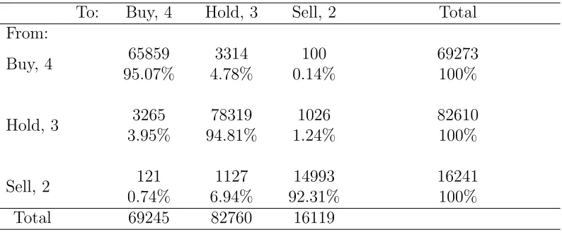
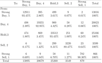
Table 1 presents the distributions of recommendation levels and the transition matrix of recommendation revisions and reiterations for brokerage houses using a three-tier rating system; and Table 2 does so for those using a five-tier rating system. Almost half of the rec-ommendations by brokerages that use three ratings are holds, 41% are buys and 10% are sells. Table 2 shows that brokerage houses that use five ratings are more optimistic—about 53% of their recommendations are strong buys or buys, and only 7% are sells or strong sells—likely reflecting that five-tier brokerage houses, which tend to be smaller, without an investment bank side, have different audiences. This means that one cannot collapse five-tier brokerage houses into three-tier ones by grouping strong buys with buys, and strong sells with sells.

22_{We show that our qualitative empirical findings are robust if we use different cutoffs (e.g., 9 or 15}

months) to identify analysts who drop coverage.

23_{This outstanding recommendation may be an actual issuance by the analyst or a carryover from a}

Table 1: Distribution of Analyst Recommendations (three-tier ratings)

Panel A. Stock Recommendation Levels Buy, 4 Hold,3 Sell, 2 Total Initiations 29910

41.00%

35862 49.16%

7172 9.83%

72944 100%

Full Sample 99159 41.13%

118626 49.21%

23291 9.66%

241076 100%

Panel B. Transition Matrix of Recommendation Revisions and Reiterations

To: Buy, 4 Hold, 3 Sell, 2 Total

From:

Buy, 4 65859

95.07%

3314 4.78%

100 0.14%

69273 100%

Hold, 3 3265

3.95%

78319 94.81%

1026 1.24%

82610 100%

Sell, 2 121

0.74%

1127 6.94%

14993 92.31%

16241 100%

Total 69245 82760 16119

For brokerage houses using a three-tier system, transitions out of buy are about as likely as those out of hold, while upward transitions out of sell are about 50% more likely. Broker-age houses using a five-tier system do not hold negative ratings for as long as those using a three-tier system—they are more likely to revise holds or sells upward, and less likely to re-vise buy/strong buy ratings down—additional indications that they tailor recommendations more optimistically. Of note, brokerage houses using a five-tier system are more likely to revise recommendations to hold than to other revisions,evenfrom strong buy and strong sell.

Table 2: Distribution of Analyst Recommendations (five-tier ratings) Panel A. Stock Recommendation Levels

Strong Buy, 5 Buy, 4 Hold,3 Sell, 2 Strong Sell, 1 Total Initiations 5476

21.51%

8137 31.96%

9960 39.13%

1519 5.97%

364 1.43%

25456 100%

Full Sample 19371 21.59%

28816 32.12%

35228 39.26%

5068 5.65%

1243 1.39%

89726 100%

Panel B. Transition Matrix of Recommendation Revisions and Reiterations

To: Strong

Buy, 5 Buy, 4 Hold,3 Sell, 2

Strong

Sell, 1 Total From:

Strong Buy, 5

12911 93.45%

395 2.86%

499 3.61%

9 0.07%

2 0.01%

13816 100%

Buy, 4 498

2.39%

19355 92.95%

900 4.32%

58 0.28%

12 0.06%

20823 100%

Hold,3 474

1.88%

869 3.45%

23512 93.43%

251 1.00%

60 0.24%

25166 100%

Sell, 2 6

0.17%

51 1.42%

299 8.31%

3220 89.47%

23 0.64%

3599 100%

Strong Sell, 1

6 0.69%

9 1.04%

58 6.70%

11 1.27%

782 90.30%

866 100%

Total 13895 20679 25268 3549 879

4

Empirical Analysis

We next present estimates of our model of analyst recommendations. We compare results from the full model (detailed in equations (1)–(4)) with those from more restricted models to emphasize the importance of both information persistence and revision frictions in the analyst decision-making process. We then investigate the indirect implications of the model for the duration of recommendations and market reactions to recommendations.

loga-rithm of the marginal likelihood of a particular model used to assess the goodness of model fit.

The ordered probit model captures an idealized analyst who employs no recommenda-tion fricrecommenda-tions and has no persistent valuarecommenda-tion informarecommenda-tion that the econometrician does not see. This model is nested in our framework when δ and ρ are set to zero. Columns 1 and 10 present parameter estimates of an ordered probit model obtained using our MCMC ap-proach and conventional maximum likelihood, respectively. The two methods yield nearly identical parameter estimates. We defer discussion of the publicly-available determinants of stock valuation to the full model.

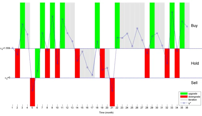
The ordered probit model fits the datapoorly. The poor fit is reflected in the large Brier score, which reveals a large discrepancy between predicted probabilities of recommendations and actual outcomes. The ordered probit model fit by maximum likelihood has a pseudo-R2 of only 2.09%. The key to the bad fit is that no matter how the model of valuation is formu-lated, it predicts far too many recommendation revisions. Figure 1 presents a sample valu-ation path: the model predicts 20 recommendvalu-ation revisions over the 36 month period, and there would be far more if we used weekly observations. In essence, while there is some persis-tence in recommendations due to persispersis-tence in public information data and quarterly arrival of earnings information (i.e., there is persistence in firm and analyst fundamentals in X), there isfar too little to generate the infrequent recommendation revisions found in the data.

Column 2 considers an idealized analyst who does not set recommendation revision fric-tions, but does gather information that the econometrician does not have, information that has persistent valuation implications. The autoregressive coefficient estimate is very high,

ˆ

ρ = 0.90, and hugely credible/significant. Incorporating this persistent information source cuts the Brier score almost in half, from 0.34 to 0.18, and it is accompanied by an enor-mous Bayes factor of exp(49740): accounting for the temporal correlation in an analyst’s information yields a vast improvement in model fit.

The high persistence in analyst information reduces the frequency of recommendation revisions. To see why, consider a stock with a valuation in month t−1 ofV_t∗₋₁ = 4.2, which is well above the Buy rating cutoff of 3.5. If an analyst receives a one standard deviation positive information shock (εt = +1), raising Vt∗ to 5.2,24 the slow decay means that it is

likely to take a long time for the valuation to drop out of the buy bin. Conversely, a one-standard deviation negative shock (εt=−1) leads to a downgrade to Hold asVt∗drops to 3.2.

However, the valuation would slowly revert, rising due to the decay of εt. Absent arrival of

24_{For the purpose of this illustration, assume thatu}

Figure 1: Idealized analyst

Recommendation cutoffs, and sample valuation and recommendation paths over a 36-month period for an idealized analyst employing a three-tier rating system whose private information is transient.

other information, the analyst would switch back to a buy recommendation after 4 months.

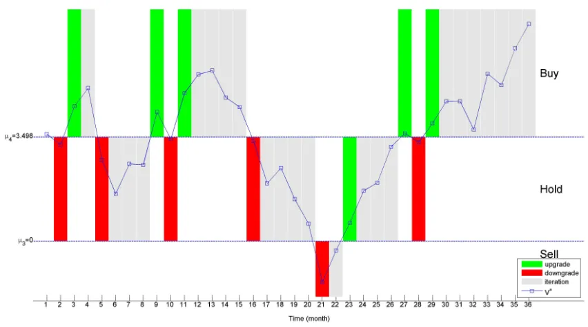
Figure 2 depicts equilibrium bins for an idealized analyst with persistent information, and it illustrates sample valuation pathsfor the same common public information valuation path and information shocks as Figure 1. Persistent information reduces the number of rec-ommendation revisions from 20 to 12. Still, the data remain badly described by an idealized analyst: Regardless of the persistence in analyst information, an idealized analyst cannot

deliver low likelihoods of recommendation revisions when the valuation is close to a ratings cutoff because small price fluctuations would lead to repeated crossings of the cutoff.

To generate the high stickiness in recommendations implicit in the small off-diagonal transition probabilities in Table 1, one needs recommendation revision frictions strategically introduced by analysts who value intertemporal consistency in recommendations. Columns 3 to 6 present estimates of such models. Column 3 presents estimates for a model with (a) only two friction parameters,δ↑ andδ↓, one for upward revisions and one for downward revisions, when (b) analysts have no persistent information. Both revision friction estimates are large

and highly significant. Model 3 has afar better goodness of fit than model 2 (Bayes factor of

Figure 2: Idealized analyst with persistent information

Recommendation cutoffs, and sample valuation and recommendation paths over a 36-month period

for an idealized analyst who has persistent information. The sample valuation path uses the same

common public information valuation path and information shocks as Figure 1.

more important driver of recommendations than persistent information. Importantly, there would be little impact on estimates were higher frequency (e.g., bi-weekly) recommenda-tion observarecommenda-tions used, because valuarecommenda-tions rarely change sharply over short windows: small changes in valuations cannot lead to successive changes in recommendations. In this way, recommendation revision frictions also capture temporal stickiness in recommendations.

Column 4 presents estimates of a model with the same two recommendation frictions,

δ↓ and δ↑, and persistent analyst information, where we now discard all publicly-available information except the constant. There is a further improvement in model fit (Bayes factor

exp(6646)), revealing that the information available to the econometrician matters far less for explaining the dynamics of recommendations than do recommendation revision frictions and persistent analyst information.

of improved model fit. These complementarities are also indicated by the huge ratios of the mean to standard deviation of parameter estimates: 85.5 for the information persistence parameter ρ, 266.9 for δ↑ and 403.4 for δ↓. This means that persistent analyst information and recommendation revision frictions capture distinct economic phenomena—persistent an-alyst information is not a proxy for an unwillingness of anan-alysts to revise recommendations. Failing to account for both sources of stickiness biases estimates significantly.

Column 6 presents estimates for our full model, in which analysts have persistent private information and recommendation revision frictions can vary with the recommendation itself and δk↑ can differ from both δk↓ and δk0_↑. That is, analysts do not need to use symmetric

recommendation revision frictions to reduce the frequency of recommendation revisions; they can tailor them to reflect other considerations (see Figure 3).

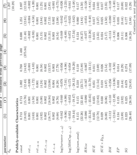
T able 3: P arameter Estimation Mo del (1) (1’) (2) (3) (4) (5) (6) (7) Recommendation Cutoffs µ5 4 . 340 (526 . 7) µ4 1 . 559 1 . 565 3 . 498 1 . 782 1 . 745 1 . 787 1 . 966 2 . 910 (384 . 3) (405 . 6) (364 . 4) (370 . 0) (339 . 3) (392 . 9) (455 . 9) (374 . 1) µ3 0 0 0 0 0 0 0 1 . 154 (140 . 33) µ2 0 P ersistence of Information ρ 0 . 895 0 . 401 0 . 389 0 . 313 0 . 609 (607 . 4) (85 . 47) (83 . 73) (66 . 15) (116 . 9) Recommendation Revisi on F rictions δ↑ 1 . 445 1 . 337 1 . 346 (974 . 0) (266 . 9) (262 . 7) δ↓ 1 . 631 1 . 525 1 . 553 (954 . 7) (403 . 4) (394 . 5)

δ5↑

1 . 174 (43 . 17)

δ5↓

1 . 324 (151 . 6)

δ4↑

1 . 336 1 . 037 (147 . 5) (165 . 3)

δ4↓

1 . 563 1 . 209 (291 . 3) (75 . 29)

δ3↑

1 . 787 1 . 509 (358 . 2) (104 . 0)

δ3↓

0 . 822 0 . 814 (91 . 11) (41 . 52)

δ2↑

T able 3 – con tin ued from previous page parameter (1) (1’) (2) (3) (4) (5) (6) (7)

δ2↓

Figure 3: Cutoff and recommendation revision friction estimates

Cutoff and recommendation revision friction estimates of the full model, in which revision frictions

are cutoff-specific, and analysts have persistent information. Cutoff-specific revision frictions, δk,↓

and δk↑, bear the same index k as cutoff µk: δk,↓ is the friction for downgrades from k to k−1,

while δk↑ is the friction for upgrades from k−1 to k.

Column 7 presents estimates for brokerages using five-tier rating systems. Most estimates are qualitatively similar to those for the three-tier system. For example, the recommendation revision friction from sell to hold is far higher than that from hold to sell. Also, the frictions from strong sell to sell and strong buy to buy arelarge relative to the sizes of the sell and buy bins (98% and 92% respectively). As a result, most revisions from strong buy and strong sell are to hold. Thus, the nature of the recommendation revision frictions that five-tier broker-ages introduce qualitatively lead them in the direction of behaving like three-tier brokerbroker-ages.

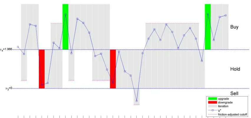
Figure 4: Reluctant analyst

Recommendation cutoffs, and sample valuation and recommendation paths over a 36-month period

for a reluctant analyst who has persistent information. The sample valuation path uses the same

common public information valuation path and analyst information shocks as Figures 1 and 2.

Also, the estimate of information persistence is far higher for five-tier brokerage houses.25

Our estimates highlight how analysts design recommendation bins and recommendation revision frictions to carefully balance reputation concerns and the desire to generate trading volume:26

• The large frictions out of strong buy and strong sell suggest that revisions to hold generate trading activity by inducing investors to unwind positions, but revisions from strong buy to buy that maintain a positive assessment, or from strong sell to sell that maintain a negative assessment do not.

• Revision frictions out of hold are small. Analysts design frictions in and out of hold

25_{One might wonder whether this high estimate could indicate that some analysts at five-tier brokerages}

act as if they were at three-tier brokerages. Such mis-classification would bias upward estimates of

information persistence. However, the many transitions from buy to strong buy and strong buy to buy indicate that any misclassification is minimal.

26_{This is consistent with analysts’ economic incentive to boost trading activities (e.g., Eames et al., 2002;}

asymmetrically, with smaller frictions out of hold, so that recommendations spend “less time” in hold, perhaps because maintained hold ratings (as opposed to revisions to hold) discourage retail investors from trading.

• Analysts are least reluctant to downgrade a stock from Hold—δ3↓ is the smallest among allδ·↓(see Table 3, Columns 6 and 7 for three- and five-tier systems, respectively). This finding is consistent with the survey evidence in Brown et al. (2015): issuing unfavor-able (Sell) recommendations may increase an analyst’s credibility with investing clients.

Even though hold revision frictions are small, the model delivers the prevalence of hold recommendations (39% for five-tier brokerages, 49% for three-tier brokerages) in three ways:

• The hold recommendation bin for five-tier brokerages is large, about 25% larger than the buy bin, and 50% larger than the sell bin.

• The estimated average firm for five-tier brokerages is roughly at the buy-hold recom-mendation cutoff, making an initial hold recomrecom-mendation likely; and the estimated average firm for three-tier brokerages is slightly above the hold bin midpoint.

• Analysts at five-tier brokerages are less likely to face revision frictions from buy or sell into hold due to the high frictions from strong sell to sell and strong buy to buy, which results in most transitions going from strong buy and strong sell straight to hold.27

Our findings make economic sense. The fact that public information available to an econometrician poorly describes recommendations makes sense—if recommendations largely reflected readily-available information, they would have modest value, and one would be hard-pressed to justify why analysts should be well-paid. That the average firm for which coverage is initiated is a hold, but closer to a buy than a sell, supports the notion that analysts tend to follow stocks that they deem to have better prospects. This is consistent with their retail clients being less likely to short-sell, so covering firms with poorer prospects generates fewer client orders. Analysts also want clients to profit from trades—a happy client is likely to trade—so analysts want there to be meaning to buy and sell recommendations, and hence are reluctant to issue such recommendations unless profits are somewhat likely to result.

27_{These estimates also give insight into where improvement in model fit occurs versus more restricted}

models of five-tier brokerages. Strong sells only comprise 1.4% of the sample, so the two frictions, δ↑ and

δ↓do not weigh transitions from strong sells heavily in the estimation. As a result, δ↑ is far larger thanδ2↑.

In turn, the large size ofδ↑ necessitates a large value for µ2 (so that transitions from strong sell to sell can

We now turn to publicly-available determinants of value. Of note, in contrast to existing findings, once we control for a reluctant analyst’s information and revision frictions, bet-ter past firm performances cease to systematically raise the analyst’s assessment: the one month lagged return enters negatively, while more distant returns enter slightly positively. Qualitatively, Column 6 reveals that a reluctant analyst has higher assessments of firms:

• for which the analyst has relatively higher estimated forecasts of earnings (vis `a vis the consensus), consistent with Womack (1996) or Jegadeesh et al. (2004).

• that have positive earnings surprise, especially in the earnings announcement window in which they are reported, as in Chan, Jegadeesh and Lakonishok (1996), Jegadeesh, Kim, Krische and Lee (2004), or Ivkovi´c and Jegadeesh (2004).

• that draw more attention from other analysts, consistent with more analysts following stocks they believe are undervalued, or possibly analysts valuing a stock’s “glamor” (e.g., Barth et al., 2001).

• that are smaller, as measured by higher sales growth (see Lakonishok, Shleifer, and Vishny (1994)) or lower book-to-price ratios (see Jegadeesh et al. 2004)).

• with less turnover, consistent with Lee and Swaminathan (2000), who argue that turnover is a contrarian sign, associated with lower returns.

• about which there is less uncertainty, as captured by forecast dispersion in earnings (see Diether et al. (2002), Zhang (2006)), lesser dispersion in recommendations, or more analyst following or higher institutional holdings.

• for which an analyst’s brokerage house has investment banking relationships, consistent with Lin and McNichols (1998), Ljungqvist et al. (2007), Malmendier and Shanthiku-mar, 2007; O’Brien, McNichols and Lin (2005), Jackson (2005), Cowen, Groysberg, and Healy (2006) and Lim (2001).

• if an analyst is at a smaller brokerage house. Analysts at smaller brokerages also issue more optimistic earnings forecasts (Bernhardt et al. (2006)), and follow smaller firms.

Quite generally, accounting for revision frictions and persistent analyst informationsharply

reduces the statistical significance/credibility of parameter estimates (relative to the ordered probit model of an idealized analyst), typically by factors of two to five, and the magnitudes of parameter estimates tend to be fall, too. Moreover, recommendation bins are large relative to the valuation consequences of variation in public information available to the econometrician, further indicating that this public information is not the primary driver of recommendations.

Robustness checks. Our econometric model of how analysts form recommendations pre-sumes that sources of heterogeneity between analysts or between the firms for which analysts issue recommendations only enter via the valuation model underlying V, and not the rec-ommendation formation model itself.28 To assess the validity of this premise, we estimate separate models for subsamples of analysts and firms where one suspects that analysts’ recommendations might vary—over time, or by brokerage house size, analyst following or analyst experience. These robustness tests revealremarkable consistency in our estimates.29 Column 1 of Table 4 reproduces estimates from the full sample. Subsequent columns present estimates for the subsamples of (S1) the second half of the sample period (2006-2010); (S2) large brokerages that on average employed at least 52 analysts over the sample period; (S3) heavily-followed stocks that were covered on average by at least 15 analysts over the sample period; and (S4) senior analysts who have been employed by the same brokerage firm for at least five years. The sample criteria were chosen so that each subsample has roughly half of the original observations.

We see true intertemporal consistency—comparing columns (Full) and (S1) reveals al-most no variation in estimates—there is no evidence that analysts have altered how they issue recommendations over this period. So, too, the subsample of larger brokerage houses (S2), and senior analysts (S4) have similar estimates. Analyst information is slightly more persistent for heavily-followed stocks, but even this difference is less than 25%, and the other structural recommendation parameters differ by far less. In sum, differences in how

vari-28_{An alternative interpretation of our findings is not that, for example, less experienced analysts (or}

ana-lysts at smaller brokerages) have higher valuations of firms than more experienced ones (or anaana-lysts at larger brokerages), but rather that less experienced analysts (or analysts at smaller brokerages) set systematically lower recommendation cutoffs, reducing all cutoffs by a constant, resulting in higher recommendations. The lack of identification between these two interpretations just reflects that recommendations reflect differences between per share valuations and cutoffs. That is, one can alternatively interpret our framework as accommodating limited heterogeneity in analyst recommendation bins, but not their recommendation revision frictions.

29_{The large ratios of the posterior mean to standard deviation for the structural parameters indicate that}

ous analysts issue recommendations are well captured by heterogeneity in their models of valuation together with a homogeneous model of recommendation formation and revisions.

Delayed Incorporation of Information by Analysts? Raedy et al. (2006) uncover in-direct evidence suggesting that it takes time for analysts to process new information, causing them to under-react to it. This leads us to modify our model to estimate the extent to which analysts fully process new information, deriving direct estimates of the amount by which an-alysts under-react to new information. We estimate a model in which, of the new information

εijt that analyst i receives about stock j at time t, he only incorporates a fraction ζ. As a

result, the valuation consequences of the analyst’s persistent information evolve according to

uijt =ρ(uij,t−1+ (1−ζ)εij,t−1) +ζεijt.

The last column of Table 5 presents estimation results for the model in which analysts can under-react to new information. Estimates indicate that analysts incorporate the vast bulk of new information immediately, incorporating all but 9 percent when it arrives. This analysis also shows that delayed incorporation of information does not drive our high estimates of per-sistence in analyst information and recommendation revision frictions. In fact, allowing for delayed incorporation of informationraises the estimate of information persistence by about one third. Moreover, changes in estimates of revision frictions are small. The estimates indi-cate that analysts are “close to rational” in their assessments of new information, and that our qualitative findings are reinforced by integrating this source of modest “irrationality”.

T able 4: Subsample Analysis Mo del (F ull) (S1) (S2) ( S 3) (S4) (6m) (9m) (15m) (dela y) Recommendation Cutoffs µ4 1 . 966 1 . 957 1 . 914 1 . 888 1 . 918 1 . 987 1 . 978 1 . 958 1 . 732 (455 . 9) (512 . 86) (238 . 5) (369 . 5) (417 . 9) (507 . 7) (489 . 7) (509 . 0) (293 . 3) µ3 0 0 0 0 0 0 0 0 0 P ersistence of Information ρ 0 . 313 0 . 309 0 . 342 0 . 388 0 . 332 0 . 289 0 . 300 0 . 321 0 . 430 (66 . 15) (47 . 96) (48 . 30) (51 . 93) (43 . 85) (48 . 71) (59 . 83) (75 . 75) (89 . 66) dela y ed in c orp orati on of information ζ 0 . 907 (336 . 7) Recommendation Revision F rictions

δ4↑

1 . 336 1 . 342 1 . 362 1 . 400 1 . 320 1 . 075 1 . 220 1 . 395 1 . 209 (147 . 5) (112 . 84) (104 . 4) (69 . 15) (67 . 89) (100 . 2) (185 . 1) (332 . 8) (220 . 4)

δ4↓

1 . 563 1 . 569 1 . 562 1 . 509 1 . 553 1 . 536 1 . 561 1 . 589 1 . 335 (291 . 3) (263 . 02) (165 . 7) (126 . 1) (138 . 1) (272 . 3) (263 . 5) (239 . 9) (256 . 1)

δ3↑

1 . 787 1 . 756 1 . 757 1 . 695 1 . 746 1 . 747 1 . 775 1 . 820 1 . 535 (358 . 2) (238 . 41) (180 . 9) (166 . 3) (174 . 1) (194 . 4) (324 . 3) (327 . 6) (375 . 3)

δ3↓