Efficient and accurate evaluation of potential energy matrix elements for quantum dynamics using Gaussian process regression

warwick.ac.uk/lib-publications

Original citation:

Alborzpour, Jonathan, Tew, David P. and Habershon, Scott. (2016) Efficient and accurate

evaluation of potential energy matrix elements for quantum dynamics using Gaussian

process regression. Journal of Chemical Physics, 145 (17). 174112.

Permanent WRAP URL:

http://wrap.warwick.ac.uk/82277

Copyright and reuse:

The Warwick Research Archive Portal (WRAP) makes this work of researchers of the

University of Warwick available open access under the following conditions.

This article is made available under the Creative Commons Attribution 4.0 International

license (CC BY 4.0) and may be reused according to the conditions of the license. For more

details see:

http://creativecommons.org/licenses/by/4.0/

A note on versions:

The version presented in WRAP is the published version, or, version of record, and may be

cited as it appears here.

Efficient and accurate evaluation of potential energy matrix elements

for quantum dynamics using Gaussian process regression

Jonathan P. Alborzpour,1_{David P. Tew,}2_{and Scott Habershon}1,a)

1_{Department of Chemistry and Centre for Scientific Computing, University of Warwick,}

Coventry CV4 7AL, United Kingdom

2_{School of Chemistry, University of Bristol, Bristol BS8 1TS, United Kingdom}

(Received 11 July 2016; accepted 4 October 2016; published online 7 November 2016)

Solution of the time-dependent Schrödinger equation using a linear combination of basis functions, such as Gaussian wavepackets (GWPs), requires costly evaluation of integrals over the entire potential energy surface (PES) of the system. The standard approach, motivated by computational tractability for direct dynamics, is to approximate the PES with a second order Taylor expansion, for example centred at each GWP. In this article, we propose an alternative method for approximating PES matrix elements based on PES interpolation using Gaussian process regression (GPR). Our GPR scheme requires only single-point evaluations of the PES at a limited number of configurations in each time-step; the necessity of performing often-expensive evaluations of the Hessian matrix is completely avoided. In applications to 2-, 5-, and 10-dimensional benchmark models describing a tunnelling coordinate coupled non-linearly to a set of harmonic oscillators, we find that our GPR method results in PES matrix elements for which the average error is, in the best case, two orders-of-magnitude smaller and, in the worst case, directly comparable to that determined by any other Taylor expansion method, without requiring additional PES evaluations or Hessian matrices. Given the computational simplicity of GPR, as well as the opportunities for further refinement of the procedure highlighted herein, we argue that our GPR methodology should replace methods for evaluating PES matrix elements using Taylor expansions in quantum dynamics simulations. C _{2016 Author(s). All article} content, except where otherwise noted, is licensed under a Creative Commons Attribution (CC BY) license (http://creativecommons.org/licenses/by/4.0/).[http://dx.doi.org/10.1063/1.4964902]

I. INTRODUCTION

Computer simulation approaches based on solution of the time-dependent Schrödinger equation (TDSE) offer an important route to modelling dynamics in quantum chemical systems;1,2 _{for example, quantum simulations of}

organic molecules,3–14_{inorganic complexes,}15_{and biological}

systems7,9,10,16,17 have all provided insight into relaxation dynamics following photochemical excitation, while other studies have highlighted the role of quantum-mechanical tunnelling or zero-point energy (ZPE) in multidimensional dynamics.18–32 The power of these simulation approaches is that they provide a direct view of real-time quantum dynamics with access to all properties of interest, such as position expectation values, electronic state populations, and branching ratios; as a result, direct solution of the TDSE is an important route to reconciling experimental observations and atomistic dynamics.

Most commonly, computational methods aimed at solving the TDSE begin with a linear expansion of the time-dependent wavefunctionψ₍q,t₎in a set of basis functions,

ψ(q,t)= n



i=1

ci(t)φi(q,t), (1)

where ci(t) is a complex expansion coefficient at time t,

φi(q,t) is the ith basis function, n is the total number of

a)_{Electronic mail: [email protected]}

basis functions, andqis the set of coordinates describing the system. In the case where the basis functions are assumed to be time-independent (i.e. φi(q,t)=φi(q)), application of the Dirac-Frenkel variational principle2,33_{gives the following}

equation-of-motion for the expansion coefficients:

˙

c=−i ~

Hc, (2)

wherecis the vector of expansion coefficients andHis the Hamiltonian matrix with elements

Hi j =⟨φi|Hˆ|φj⟩=⟨φi|Tˆ+Vˆ|φj⟩. (3)

While this time-independent-basis approach has been employed extensively, most notably in studying gas-phase collisional and scattering processes,34–42_{application to larger}

systems is implicitly limited because the static basis set must, by definition, span the entire configurational space available to the system at all times; this leads to the well-known exponential scaling with dimensionality.

Methods for solving the TDSE with time-dependent basis functions can circumvent this “curse of dimensionality”, albeit with the introduction of new computational challenges. Here, the basis functions are parameterized by a set of time-dependent variables, and the equations-of-motion governing the time-evolution of these parameters can be determined in two different ways: (i) variationally, using the Dirac-Frenkel variational principle, or (ii) non-variationally, using approximate evolution equations. Of the former class,

the multiconfigurational time-dependent Hartree (MCTDH) method is perhaps the most well known;1,4,5,43,44this strategy employs fully variational treatment of the time-dependence of the basis expansion coefficients and the basis functions themselves, which are described as Hartree products of low-dimensional basis functions (typically represented using a discrete variable representation (DVR) or similar1,2,45). The MCTDH methodology has enjoyed enormous success in describing photochemical dynamics in small molecules such as fulvene46 _{and pyrazine,}47 _{as well as model systems}

of condensed-phase environments.48 _{However, the MCTDH}

strategy requires that the potential energy surface (PES) describing the system must be written as a “sum of products” for the time-propagation to be computationally tractable; while strategies have been developed to cast PESs into the required form,1,49 _{this prescription restricts the use of}

MCTDH in more general “on the fly” schemes for quantum dynamics which directly couple to ab initio electronic structure calculations. Building on the success of MCTDH, the Gaussian-MCDTH (G-MCTDH5) method also employs the time-dependent variational principle to evolve the basis functions, although in this case some of the degrees-of-freedom in each Hartree product basis function are treated as Gaussian wavepackets (GWPs); taking this development to its natural conclusion, the variational multiconfigurational Gaussian (vMCG13,14,50–53_{) method employs GWP products}

for all degrees-of-freedom, again employing variational propagation to evolve the basis set. The vMCG method is more generally applicable than MCTDH in “on the fly” schemes, coupling ab initioelectronic structure calculations and basis propagation, although not without problems; for example, linear dependence in the GWP basis set, as well as the growth of the matrix equations required for propagation, means that convergence with respect to basis set size can be challenging.

In methods which employ non-variational evolution of the basis set, the most common approach is to select computationally tractable equations-of-motion to describe the evolution of the parameters describing the basis functions, while using the time-dependent variational principle to describe the evolution of the associated expansion coefficients.7–10,12,19,21,31,32,54–60 _{The resulting}

equation-of-motion for the expansion coefficients is

˙

c=−i ~S

−1 _H−i

~S˙c, (4)

whereHis defined in Eq.(3), the time-derivative matrix is

˙ Si j =



φi

∂φj dt



, (5)

and the overlap matrix is

Si j=⟨φi|φj⟩. (6)

Because of the non-variational nature of the evolution of the basis functions, such methods do not, in general, conserve energy (unless a complete basis is used19); however, norm conservation for Hermitian Hamiltonian operators is preserved by Eq. (4). Within this framework, by far the most common basis functions employed are GWPs, as in vMCG; for an

f-dimensional system, these are typically of the form

φi(q,t)= f



κ=1

(₂ακ

i

π

)1/4

e−ακi(qˆ

κ_−qκ

i(t))2+i p

κ

i(t)(qˆ

κ_−qκ

i(t)), ₍₇₎

where we have adopted atomic units (_~=1). Here, the GWP basis function for each degree-of-freedom is parameterized by a position q_iκ₍t₎ and a momentum pκ_i(t₎, as well as a width parameter ακ_i; in what follows, we assume for simplicity that we are dealing with the common case of “frozen” GWPs, where the width parameters are fixed,61

although we note that the methods discussed throughout this article are equally applicable in the “thawed” GWP case.

The popularity of GWP basis functions in non-variational wavefunction propagation methods originates in their appealing connection to classical trajectories.2,61,62 In particular, for a single basis function φi(q,t), it is straightforward to show that the expectation values of position and momentum for degree-of-freedom κ are simply qκ_i(t) and pκ_i(t), respectively; in other words, these parameters can be viewed as defining a single phase-space point, just as in classical mechanics. Besides this connection to classical mechanics, a further important aspect which is important to note is that GWPs arelocalisedin configuration space; this feature is relevant to the current work and will be described further below. Primarily as a result of the computationally appealing characteristics of GWPs, these basis functions have formed the foundation of several approaches to modelling quantum chemical dynamics. For example, the ab initio multiple spawning (AIMS7–10,54–57) method has been employed to model photochemical dynamics in the gas-phase and the condensed-phase, while the coupled coherent states (CCS31,32,58,60) approach, and the more recent multiconfigurational Ehrenfest (MCE59_{) methodology, have}

been benchmarked against a range of model problems and molecular systems. In our own recent work, we have shown how the common problem of linear dependence in GWP basis sets can be circumvented using adaptive strategies,19

and we have also proposed a trajectory-guided strategy which employs classical dynamics to sample relevant regions of GWP phase-space for subsequent solution of the TDSE.21

Regardless of the quantum simulation approach taken (variational or non-variational) and the type of basis function employed (e.g. GWPs or DVRs), all basis-set based approaches to solving the TDSE have a common computational bottleneck beyond the explicit treatment of high-dimensionality, namely the calculation of matrix elements of the potential energy operatorV(qˆ). While explicit analytical calculation of matrix elements of the kinetic energy operator, ˆT, is generally straightforward (particularly if using rectilinear coordinate systems), the determination of potential energy matrix elements is much more challenging. In particular, the PE matrix element for basis functionsφi(q,t) andφj(q,t)is given as

Vi j=



dqφ∗_i(q,t)_Vˆ_{φj(q,t). (8)}

in a simple analytical form, exact evaluation of this integral is generally impossible. This is clearly the case if one is interested in performing quantum dynamics simulations “on the fly,” linking evolution of the TDSE to PES evaluation usingab initioelectronic structure calculations.

In the absence of a simple analytical PES, the most common approach to calculating matrix elementsVi jis to use a Taylor expansion,13,14,51,52,63 _{typically taken around either}

the position q_i(t)of one of the GWPs or the position of the GWP arising as the product of the two separate GWPs; as discussed in detail below, this Taylor expansion is typically truncated at the second-order (Hessian matrix) term or lower. While this approach is generally well-founded, based on the locality of GWPs, it is not without its shortcomings. For example, calculation of the Hessian matrix using ab initiomethods can be computationally expensive, limiting the appeal of methods based on second-order Taylor expansions. Furthermore, the implicit assumption of the second-order Taylor expansion, that the PES is well-characterized as a harmonic expansion around a single configuration, can clearly be limited in accuracy, depending on the characteristics of the underlying PES. Finally, in the case where expansion around the position of the product GWP is employed, we note that this can require O(n2) evaluations of the PES (and possibly the derivative and Hessian matrix, depending upon the order of Taylor expansion) to evaluate the full PE matrix; however, the total number of PES evaluations can be reduced by integral pre-screening based on the magnitude of the overlap Si j between GWPs. In any case, it is clear that the range of applicability of the Taylor expansion approach, as well as its ultimate accuracy (as demonstrated below), can be limited; in this article, we propose an alternative.

In this work, we explore a new approach to calculating PE matrix elements in quantum dynamics simulations; while our approach is presented in the context of GWP-based strategies, we emphasize that it is generally applicable to any quantum dynamics method in which the basis functions are written as a Hartree product (an almost universal assumption). In particular, we propose using Gaussian process regression (GPR64–71_{) to calculate PES matrix elements, using only}

single-point calculations performed along the trajectories

qi(t) of time-dependent basis functions. In Section II, we first describe current approaches to calculating PES matrix elements, with a specific emphasis on simulations using GWP basis functions; we then describe our proposed GPR-based approach to approximating PES matrix elements for GWP basis sets. In Section III, we investigate the accuracy of different matrix element approximations for benchmark 2-, 5-, and 10-dimensional problems. Our results demonstrate convincingly that GPR should be employed as the method-of-choice in evaluating PES matrix elements in GWP-based quantum dynamics simulations; in particular, our GPR-based method only requires single-point PES evaluations at each GWP basis function, is generally more accurate than Taylor expansion methodologies, and does not require the (usually expensive) calculation of the Hessian matrix. Overall, GPR is therefore expected to find use in further development of “on-the-fly” quantum dynamics strategies.

II. THEORY

Before introducing our GPR methodology for evaluating PES matrix elements, we set the context for this development by first describing the most common methods employed in previous studies. We emphasize here that our interest is particularly in quantum dynamics methods based on GWP basis sets; furthermore, we will also outline the advantages and disadvantages of the PES matrix element calculation methods described below in the context of prospects for combining these methods with ab initioelectronic structure methods in “on-the-fly” propagation schemes.

As an aside, we note that the focus of this proof-of-concept article is on assessing the viability of GPR in calculating PES matrix elements. As a result, we focus on modelling quantum dynamics in benchmark systems for which an analytical PES is available, such that we can compare approximatedVi j elements to their exact counterparts. Furthermore, we focus on modelling systems with a single ground-state PES; prospects for extension to non-adiabatic PESs are discussed later and will be left for future development.

A. Taylor expansion methods

A well-known and widely exploited property of Gaussian basis functions is the fact that a product of two Gaussian functions is itself also a Gaussian function. In the case of GWPs, using the definition of Eq. (7), the product of two GWPs (with one taken as the complex conjugate, following Eq.(8)) is

φ∗

i(q)φj(q)

=

f



κ=1

(₄ακ

iα

κ

j

π2

)1/4

×e−ακi+ακj(qˆκ−q¯κ)2+i(pκj−pκi)qˆκ+i pκiqκi−i pκjqκj−ακi(qκi)2−ακj(qκj)2,

(9)

which is a complex Gaussian function centered at

¯ qκ=

ακ

iq

κ

i +α

κ

jq

κ

j

ακ

i +α

κ

j

. (10)

In the case of frozen GWPs with equal widths, as commonly employed in a number of GWP-based strategies, the product centre ¯qκsimply becomes the mean value of the coordinates of the two constituent GWPs.

The fact that the GWP products in Eq.(8)are localised around ¯q=₍q¯1_,q¯2_{, . . . ,q¯}f

)suggests that we can make progress in approximating PES matrix elements using a Taylor expansion around ¯q, such that

V(q)≃V(q¯)+ f



κ=1

(qˆκ−q¯κ)_∂∂V qκ

+1

2 f



κ, µ=1

(qˆκ−q¯κ) ∂ 2_V

∂qκ∂qµ(qˆ

µ_−q¯µ

), (11)

where the derivatives and the Hessian matrix are evaluated at ¯

Vi j=⟨φi|Vˆ|φj⟩

≃V(q¯₎Si j+ f



κ=1

⟨qκ⟩i j−q¯κSi j ∂V

∂qκ

+1

2 f



κ, µ=1



⟨qκqµ_{⟩i j}−q¯κ_⟨qµ_{⟩i j}−q¯µ_⟨qκ_{⟩i j}+q¯κq¯µSi j 

× ∂

2_V

∂qκ∂qµ, (12)

where

⟨qκ_{⟩i j}=_⟨φi|qˆκ|φj⟩ (13)

and

⟨qκqµ⟩i j=⟨φi|qˆκqˆµ|φj⟩, (14)

which can both be evaluated analytically for GWP basis functions. The Taylor expansion form of Eq. (12) can of course be truncated at a lower order than the quadratic term, leading to a series of methods for approximating the matrix elementsVi j. For example, truncating at the zero-order terms gives

Vi j ≃V(q¯)Si j, (15)

which is the “saddle point” approximation commonly employed in the AIMS simulation strategy. For brevity in later discussion, we refer to Eq. (15) as the MT0 approximation (mid-point Taylor expansion to zero order), Eq. (12)is the MT2 approximation, and it follows that the MT1 approximation is defined as

Vi j≃V(q¯)Si j+ f



κ=1

⟨qκ⟩i j−q¯κSi j ∂V

∂qκ. (16)

Application of the MT0-2 approximations requires calculation of the potential energy and, possibly, the first- and second-derivatives at the mid-point coordinate of each pair of GWPs; as a result, this requires at mostn+n₍n−1₎/2 PES evaluations to evaluate the full PE matrix for n GWP basis functions. However, this value can be reduced by further exploiting the locality of GWPs; in particular, if|Si j|≤ϵ, whereϵis a small cutoffparameter, then it can be assumed that the GWPs are sufficiently well-separated that the corresponding PE matrix elements are zero. Ifab initioelectronic structure calculations are to be employed in calculating V(q₎, this pre-screening procedure can clearly reduce the total number of PES evaluations and reduce computational cost.63 _Furthermore,

there is clearly a progression in computational expense as one moves from MT0 to MT2; in particular, calculation of the Hessian is often an expensive operation withinab initio electronic structure methods.

An alternative to the mid-point Taylor expansion approach described above is to instead consider Taylor expansion around one of the GWP basis functions associated with the matrix element Vi j; this approach has found extensive use within G-MCTDH and vMCG calculations. Shifting the centre of the Taylor expansion toqi(t), and again truncating at second-order at most leads to three furtherVi japproximation methods,

Vi j ≃V(qi)Si j, (17)

Vi j≃V(qi)Si j+ f



κ=1

⟨qκ⟩i j−qκ_iSi j ∂V

∂qκ_i, (18)

Vi j≃V(qi)Si j+ f



κ=1

⟨qκ⟩i j−qκiSi j ∂V

∂qκ_i

+1

2 f



κ, µ=1



⟨qκqµ⟩i j−q¯κ⟨qµ⟩i j−q_iµ⟨qκ⟩i j+q_iκq¯µSi j 

× ∂

2_V

∂q_iκ∂q_iµ. (19)

We refer to Eqs.(17)-(19)as, respectively, the GT0, GT1, and GT2 approximations (i.e. Gaussian-based Taylor expansion to zero-, first-, and second-order). In passing, we note that, because the Taylor expansion in GT0-2 is taken around a GWP in the current basis set rather than at a mid-point as in MT0-2, the total number of PES evaluations (including possibly first-and second-order derivatives) is n; as a result, evaluation of a full PE matrix using GT0-2 should be computationally cheaper than MT0-2, although both sets of methods may require the (potentially costly) calculation of the Hessian matrix. Furthermore, it is clear that one could equally perform the Taylor expansion around either qi(t) or qj(t); in what follows, we adopt the standard procedure of averaging the PES matrix elementVi jover both expansions, noting that this does not require any additional PES evaluations.

B. Shepard interpolation

An approach to evaluating PES matrix elements which spans the Taylor expansion method above and the GPR methodology below is Shepard interpolation.52,72–75 Here, the PES is approximated as a linear combination of Taylor expansion terms,

V(q)≃ M



i=1

ci(q)Ti(q). (20)

The sum of Eq.(20)is taken over a set of M configurations {qi}at which second-order Taylor expansionsTi(q)have been determined; we note thatTi(q)has exactly the same form as given previously in Eq.(11). The coefficientciassociated with each Taylor expansion is typically chosen to be of the form

ci(q)= |

q−qi|−p

M

k=1|q−qk|−p

, (21)

where p is an even integer (typically 4). Overall, Eq. (20)

by continuously adding new data points as new regions of configuration space are sampled.76,77

However, the Shepard interpolation method embodied in Eqs. (20) and (21) has two important drawbacks which have curtailed its use as a general strategy for calculating PES matrix elements in quantum dynamics simulations. First, construction of the PES of Eq. (20) requires calculation of the Hessian at each of the expansion points (or at least at one initial point if Hessian update schemes are used53_);

as noted already, this calculation can be computationally expensive if using ab initio electronic structure calculations to describe the PES. Second, the weighting functions of Eq. (21) are themselves functions of configuration space, such that analytical integration of the Shepard PES over basis functions in quantum dynamics simulations is generally non-trivial. Indeed, most likely as a result of this second point, a previous application of Shepard interpolation within the setting of quantum dynamics simulations actually employed Taylor expansion of the interpolated PES of Eq. (20)

around the GWP centres,52 rather than direct evaluation; in other words, although Shepard interpolation has been used to generate an interpolated PES, evaluation of PES matrix elements in quantum dynamics calculations using Shepard interpolation has still relied on the Taylor expansion methodology outlined above. As a result, and because of our interest in developing a computationally efficient scheme which circumvents calculation of the Hessian, we do not consider Shepard interpolation further in this work.

C. A new approach: Gaussian process regression

We are now in a position to describe the GPR approach employed in this work. GPR, often referred to as kriging,64,66–68 _{is broadly representative of a class of}

machine-learning algorithms for regression of complex hyper-surfaces based on limited input data. For example, recent work has employed Gaussian process methods65 to achieve machine-learning of accurate PESs describing both atom and molecular chemical systems; the resulting Gaussian approximation potential (GAP69–71) or kriging method64,66–68 offers a route to performing molecular simulations on PESs which approximate ab initioelectronic structure, albeit at a much lower computational cost. Moving away from PES interpolation, machine learning methods such as kernel ridge regression, Bayesian inference, and artificial neural networks, have found application in relating ab initio atomization energies to simple molecular descriptors such as atomic partial charges,78_{in learning optimized}

exchange-correlation functionals for density functional theory (DFT) calculations,79,80 and in learning accurate interatomic PESs for large-scale molecular simulations.81Within the same field of chemical dynamics, a particular interest of the present work, machine-learning in the form of a support vector machine has also found application in determination of optimal dividing surfaces for transition state theory calculations.82

In this work, we present the first exploration of the use of GPR in the calculation of PES matrix elements for quantum dynamics simulations. GPR has its origin in Bayesian inference approaches65_{and, in the current context, represents}

a strategy for interpolating a PES given the values of the PES at a set of reference points. Using GPR with a Gaussian covariance kernel, the interpolated PES is written as a linear combination of Gaussian terms,

V(q)≃ M



k=1

wke−γ|q−qk|

2

. (22)

Here, M is the number of reference GPR configurations, at which it is assumed that we have calculated the value of the PES, and γ is a parameter which defines the length-scale of the Gaussian functions. Given M unknown weights and M values of the PES, the determination of the weights wk in the interpolated PES requires solution ofM simultaneous equations; here, we solve

Aw=b, (23)

whereAis anM×M covariance matrix with elements

Ai j=e−γ|qi−qj|

2

+σ2_δ

i j, (24)

and b is the vector of known PES values at the reference configurations,

bi=V(qi). (25)

In this work, Eq. (23) is solved using a standard LU-decomposition method, as implemented in the LAPACK library.83The parameter σ can be viewed as an estimate of the error within the calculated PES values; in the case of the analytical PESs considered here, this parameter can be eff ec-tively viewed as a regularisation parameter which stabilises the solution of Eq.(23). Furthermore, we treat the parametersσ andγas simple variables which are chosen at the outset of our quantum dynamics simulations; as an alternative, one could, of course, optimize these parameters by minimizing the predic-tion error in a test-set of configurapredic-tions, as discussed later.

We note that, in Eq.(22), we use the Euclidean distance in coordinate space as the measure of the distance between pointsqandqk. More generally, this choice is not expected to be optimal; for example, in the context of quantum dynamics simulations, the frequently encountered coupling between multiple degrees-of-freedom in rectilinear coordinates, such as Cartesian or normal mode space, suggests that a better choice of coordinates for describing the PES should aim to employ degrees-of-freedom which decouple motion amongst different coordinates.18,84 _{For example, recent work has highlighted}

the use of local molecular descriptors in GAP simulations of silicon and water,69–71 _{while a range of}

dimensionality-reduction algorithms might be equally employed to derive appropriate (generally non-linear) coordinates.85,86_{Given the}

success of the GPR approach demonstrated below, a line for future research will clearly be developing methods for optimising coordinate representations; simple Cartesian coordinates suffice for this proof-of-concept study.

from which we will construct our GPR interpolation surface. Once the weights have been determined using Eq. (23), the PE matrix elements can be evaluated using the GPR surface,

Vi j=



dqφ∗_i(q,t₎Vˆφj(q,t),

=

M



k₌1 wi



dqφ∗_i(q,t₎e−γ|q−qk|2φ j(q,t),

=

M



k₌1 wi

f



κ=1



dqκ₍φκ_i(qκ,t₎₎∗e−γ(qκ−qκk)2₍φκ j(q

κ_,t

)),

=

M



k₌1 wi

f



κ=1

I_kκ, (26)

where we have exploited the fact that both the GWPs and the Gaussian terms of Eq. (22) are a simple product of one-dimensional terms, one for each of the f degrees-of-freedom. The one-dimensional Gaussian integral for GPR reference point kand degree-of-freedom κ, namelyIκ_kcan be determined analytically, giving

I_kκ=N

(π

a

)1/2

e(b+i c) 2

4a +(d+ie), ₍₂₇₎

where the coefficients are

a=ακ_i +ακ_j+γ,

b=2ακ_iq_iκ+2ακ_jqκ_j +2γq_kκ,

c=pκ_j−pκ_i,

d=−ακ_i(q_iκ₎2−ακ_j(qκ_j)2−γ₍qκ_k)2,

e=pκ_iq_iκ−pκ_jqκ_j,

N=

(₂ακ

i

π

)1/4(₂ακ

j

π

)1/4

.

(28)

Overall, once the GPR weights have been determined, the entire PE matrix can be evaluated analytically using the GPR approximation of Eq. (22); this evaluation is a simple sum-of-product terms which are straightforward to evaluate.

The method described above employs PES evaluations at the GWP positions at each time-step, constructs the GPR weights, and then uses Eqs. (22),(26), and(27)to evaluate the full PE matrix, as required for evolution in Eqs. (2)

or(4). However, we note here that this is the simplest possible implementation of GPR that one could imagine in the context of GWP-based quantum dynamics simulations; in particular, at least two further refinements are possible within this scheme. First, there is clearly an opportunity to recycle previous PES evaluations within the GPR scheme. Specifically, the sum over reference configurations in Eq. (22) is not restricted to run over the nGWPs in the basis set at any given time; instead, one can easily construct a database of configurations and the corresponding PES value which can be reused in the evolution of the PE matrix elements. In this way, one can “grow” a GPR interpolation during the course of a quantum dynamics simulation, a strategy that has been previously explored in the context of Shepard interpolation.76,77 Furthermore, we note the statistical basis of GPR allows evaluation of an error estimate for the interpolated PES at any new configuration;65 as a result, as GWPs evolve according to either variational

or non-variational equations-of-motion, one can assess how accurate the GPR interpolation is at a point qi(t) and use this information to assess whether or not additionalab initio calculations are required. As a second refinement of the basic GPR strategy outlined here, we note that the determination of the GPR weights (Eq.(23)) can be modified to include forces as target values, rather than just PES values. Importantly, beyond that associated with solving a larger matrix equation, this strategy will typically not require significant additional expense with regards to PES calculations; in particular, if non-variational GWP evolution strategies are employed, such as classical trajectories, the forces at each GWP centreqi(t)will alreadybe available. Overall, both of these strategies might be expected to further improve the GPR results although, as we show below, our basic strategy is already impressively accurate.

Finally, before considering the performance of GPR as a tool for calculating PE matrix elements, it is worth highlighting the relative merits of this approach compared to the Taylor-expansion-based methods described above. First, GPR does not require calculation of the Hessian matrix, as is often required in the second-order Taylor expansion methods commonly employed in GWP simulations. Second, as described above, GPR uses input (PES values and, possibly, forces) which is already routinely calculated in GWP evolution, particularly if classical equations-of-motion are employed to propagate GWPs; in other words, no additional PES evaluations are required to evaluate the full PE matrix, in contrast to the MT0-2 methods described above. Third, GPR does not make any implicit assumption about the local shape of the PES, beyond the assumption that the PES is a smoothly varying function of the chosen coordinates; for example, the GT2 and MT2 methods implicitly assume that the PES can be expressed using, at most, quadratic terms. Fourth, as highlighted above, the GPR methodology can be adapted such that PES reference points are drawn from a stored database of configurations which “grows” during the simulation; while the same approach is true of the Shepard interpolation method, we again note that direct evaluation of PE matrix elements with Shepard interpolation is not as straightforward as in the case of GPR. Finally, and perhaps most importantly for the more widespread adoption of GPR, we note that this strategy is straightforward to implement in any scheme in which the time-dependent wavefunction is expressed using Hartree product basis functions; such basis functions are almost universally employed, most notably in the MCTDH methodology.

Overall, therefore, GPR clearly possesses many desirable properties with regards to automated construction of PESs appropriate for quantum dynamics simulations. The only remaining question is its accuracy relative to strategies currently in use; we now turn to addressing this question.

III. APPLICATION, RESULTS, AND DISCUSSION

systems for which an analytical PES is available, such that the corresponding PE matrix elements can be exactlyevaluated for our GWP basis functions. As a result, we can assess the accuracy of the different PE matrix approximation methods by comparing individual elements Vi j to the exact results. This comparison can, in principle, useanyset of GWP basis functions; for example, one can imagine randomly placing GWP basis functions and then comparing both the analytical and approximated PE matrix elements. However, the danger of this approach is that one might sample GWP basis function positions which are not representative of positions sampled in a typical quantum propagation. For example, in the worst case, sampling GWP positions which are far apart (according to, say, a Euclidean distance) may lead to many of the off -diagonal elements of the PE matrix to simply be close to zero in both the analytical and approximated PE elements; this “false positive” effect would lead to an overestimation of the accuracy of the different approximation methods (although we also consider this point further below in order to address the possible influence of the GWP propagation on the predictive accuracy of GPR).

Instead, we choose to use classical molecular dynamics (MD) trajectories to propagate a GWP basis set, with initial conditions sampled according to the properties of the initial wavefunction; this approach has been employed extensively in, for example, the AIMS approach, as well as in our own recent work. Specifically, in all of the calculations reported below, the initial wavefunction for propagation is assumed to itself be a GWP, ψ₍0₎=φI(q); initial conditions for the n GWP basis set trajectories are subsequently generated by Wigner sampling from φI(q) and the entire basis set is then propagated using standard classical MD. Along this trajectory, we periodically calculate the PE matrix elements Vi j which would be required for the full quantum evolution of the complex expansion coefficients according to Eqs. (2) or (4). These PE matrix elements are calculated analytically, as well as using the MT0-2, GT0-2, and GPR approximations; the accuracy of each approach can then be directly evaluated along the trajectory as the root-mean-square error (RMSE) between the exact and approximated PE matrix elements.

The model chosen for this study is a double-well coupled to a set of harmonic oscillators; the PES is

V₍q₎= 1

16ηq

4 1−

1 2q

2 1+

f



k=2

 1 2q

2 k+bq1q2k



, (29)

whereb=0.05 andη =1.3544. This model has been studied previously by several quantum dynamics methods, including CCS60 _{and MP/SOFT.}22 _{Notably, this is a challenging PES}

to model due to the coupling between the harmonic degrees-of-freedom and the tunnelling coordinate associated with the double-well; this coupling means that the effective potential energy along the tunnelling coordinate is asymmetric and, as a result, requires accurate evolution of a large GWP basis set to obtain converged results. Furthermore, we note that this potential exhibits anharmonicity in all degrees-of-freedom, and is therefore more generally representative of typical molecular systems than a simple harmonic model. For the

purposes of this article, Eq. (29) is an ideal test case; PE matrix elements can be analytically evaluated, yet this model is complex enough to be representative of “typical” quantum dynamics problems, in this case relating to tunnelling.

As the first test of the proposed GPR method, we consider the two-dimensional version of Eq. (29) (f =2). Here, n=200 GWP basis functions were propagated classically, with initial positions and momenta sampled from the Wigner distribution of the initial wavepacket. The initial GWP was positioned at qk =0 for all degrees-of-freedom k, except q1=−2.5; the momenta were pk =0 for all degrees-of-freedom. The GWP basis functions were propagated with a time-step of∆t=10−3_{a.u. for a total timeT =10 a.u.}

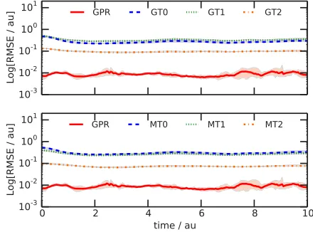
Figure 1 shows the time-dependence of the root-mean square error (RMSE) determined between the different PES matrix element approximations (GT0-2, MT0-2, and GPR) and the PES matrix elements evaluated analytically at each time; in these calculations, we usedγ=0.1 as the GPR width parameter andσ2=10−8. At each time-point, we evaluate

RMSE=

       1 n2

n



i,j=1



Re₍V_{i j)}c −Re₍V_{i j}an₎2

+

Im₍V_{i j)}c −Im₍V_{i j}an₎2       

1/2

, (30)

whereV_{i j}candV_{i j}anare, respectively, the PES matrix elements evaluated using the calculation methods discussed herein, and the analytical matrix elements; furthermore, we note that we explicitly compare both real and imaginary parts of the matrix elements.

The results of Fig. 1 unequivocally demonstrate that our GPR approach for evaluating PES matrix elements is immediately more accurate than any of the alternative methods tested. Compared to both GT0-2 (Fig. 1 upper panel) and

MT0-2 (Fig.1lower panel), we find that the GPR approach is at least an order-of-magnitude more accurate in reproducing the PES matrix elements without requiring calculation of the Hessian matrix at any point and only using PES evaluations at thenGWP positions at each time-step (without recycling previous PES data). Furthermore, this performance is maintained throughout the course of the calculation; there is no point at which any alternative method is more accurate.

However, we note that one potential disadvantage of the GPR method is the choice of width parameter γ; the simulation results of Fig. 1 were obtained using γ=0.1. The effect of γ on the accuracy with which the analytical PES matrix elements are reproduced is illustrated in Fig. 2. Encouragingly, we find that the overall accuracy of the GPR approach is relatively insensitive to the exact value of γ for this 2-D model; for 0.02≤γ≤0.4, the average error in the PES matrix elements is always much lower than the next best performing approximation methods, as shown by comparing the results of Fig.2to Fig.1. Further increase toγ≥0.5 then leads to much larger variation in the PES matrix elements, presumably because the interpolation of the PES between GWPs becomes inaccurate beyond the typical radius of each individual GWP. The results of Fig.2clearly demonstrate that there is a window of reasonable values of γ; however, we also note that further refinements of the choice of γ could rely on the fact that an error estimate of the GPR accuracy at an arbitrary configuration is readily calculable.65_{As a result,} γ could be selected by minimizing the PES approximation error at a set of test configurations; this adaptive scheme for modifyingγwill be explored in our future applications of this GPR methodology.

At this point, we stop to consider a further question relating to the results of Fig. 1: is it possible that the scheme by which we are generating GWP positions and momenta, namely by Wigner sampling from the initial wavefunction then using classical trajectories, is biasing our results? There is a simple route to assessing the potential impact of the imposed correlation in our GWP basis set, namely to completely remove the role of initial sampling and subsequent dynamics by generating independent sets

FIG. 2. Variation of the root-mean-square error (RMSE; Eq.(30)) between exact and GPR PES matrix elements as a function of the GPR width parameter

γ. Note that the error bars are comparable to the symbol size.

of GWP positions and momenta which are uniformly and randomly distributed throughout phase-space. Here, instead of time-evolution of the basis set, we randomly re-sample the positions and momenta of all GWPs at every time-step before calculating the GPR approximation to the PES matrix elements; specifically, positions and momenta were generated such thatqk ∈[−3,+3]andpk∈[−0.5,+0.5]for each degree-of-freedom k. The comparison between the trajectory-based GWP sampling and the randomly generated GWP basis set is shown in Fig.3. We note that, in this case, we illustrate the fractionalerror in the PES matrix elements, defined as

FE=        1 n2

n



i,j=1

     

Re(V_{i j}c)−Re(V_{i j}an)

Re(V_{i j}an)      

2

+(1−δ_{i j)}      

Im(V_{i j}c)−Im(V_{i j}an)

Im(V_{i j}an)      

2_

     

1/2

, (31)

and we also note that the imaginary contribution is excluded in the case of diagonal elementsi=jbecause these components are implicitly zero for the standard configurational PES of Eq.(29). The reason for considering the fractional error is that the average magnitudes of the PES matrix elements generated in the random and trajectory-based sampling methods are different; in particular, we find that the off-diagonal matrix elements generated by the random sampling approach are much smaller in magnitude than those generated by the trajectory-based method. As such, the absolute RMSEs calculated for the various approximation methods using Eq.(30)are generally lower for the randomly sampled basis sets, preventing direct comparison of the two basis generation methods; considering the fractional values scale the errors to account for this artificial discrepancy.

Figure 3 clearly demonstrates that the significant improvement of the GPR approach over the Taylor expansion

methods is not related to the basis propagation; the accuracy is similar whether trajectory-based sampling or random sampling of GWP basis functions is employed. The same is found to be true of the GT0-2 and MT0-2 methods; there is no appreciable difference in the PES matrix element approximation accuracy between trajectory and randomly sampled basis sets. These results are highly encouraging, suggesting that the performance of the GPR methodology is independent of the chosen propagation method. As a result, implementation of GPR matrix element evaluation within the framework of alternative quantum dynamics schemes, particularly the v-MCG method,14 _{would be expected to}

provide significant computational savings given that GPR (in its most simple implementation demonstrated here) does not require any information beyond PES values at a set of distinct configurations.

A. Role of PES dimensionality

As a further assessment of the GPR approach, we consider the performance in approximating PES matrix elements for higher-dimensional models; in particular, we consider f =5 and f =10 in Eq. (29). These represent much more challenging prospects than the 2-dimensional case considered above, principally because the volume of configuration space increases exponentially with the dimension of the system; this presents a particular challenge to interpolation methods such as GPR, for which the accuracy of PES approximation might be expected to decrease due to insufficient coverage of interpolation points. 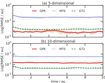We also note that, from now on, we only focus on comparing GPR to those methods which are most commonly used in GWP-based quantum dynamics simulations, namely MT0 and GT2.

Figure4illustrates the RMSE in the PES matrix elements for the f =5 and f =10 model potentials in Eq.(29); these

FIG. 4. Root-mean-square error (RMSE; Eq.(30)) between exact and ap-proximate PES matrix elements calculated during propagation of n=200 GWPs on the f=5- and f=10-dimensional PES of Eq.(29). Both panels compare the performance of GPR to the MT0 and GT2 Taylor expansion methods; in each case, the line illustrates the average over five independent simulations starting with different random initial sets of GWP basis functions and the shading illustrates the minimum and maximum variation amongst these five calculations at each time-step.

simulations were performed in exactly the same way as the 2-dimensional simulations above, except that the GPR width parameter was chosen asγ=0.05. In the case of the 5-dimensional model, GPR clearly outperforms the Taylor expansion methods in reproducing the exact PES matrix elements; as expected based on the considerably higher dimensionality of this system, the overall accuracy of the GPR PES matrix approximation decreases compared to that of the 2-dimensional model, but is still clearly better than MT0 and GT2. As the dimensionality is increased further tof =10, the accuracy of GPR decreases; however, we note that it is still more accurate than MT0 and comparable in accuracy to GT2, despite GPR requiring much less input information about the PES than either of these Taylor expansion approaches.

For completeness, Fig. 5 illustrates the fractional error in the same set of simulations as illustrated in Fig. 4. As noted above, the fractional error better accounts for the fact that the magnitude of the PES matrix elements changes with dimensionality, both as a result of implicit changes in Eq. (29) and as a result of the fact that the PES matrix becomes increasingly sparse as the dimensionality increases. However, Fig. 5 illustrates the same trend as Fig. 4; GPR is generally better than, or at the very least comparable to, the Taylor expansion methods without requiring either the Hessian (as in GT2) or additional PES evaluations (as in MT0). Furthermore, we note that, when one considers fractional error rather than standard root mean-square error, the advantage of GT2 over GPR is removed; in other words, for the higher-dimensional f =10 model, all three methods are comparably accurate when scaled by the magnitude of the PES matrix elements, primarily due to the fact that the off-diagonal PES matrix elements become much smaller in magnitude (and therefore challenging to accurately evaluate) as dimensionality increases.

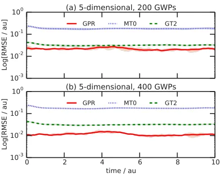
FIG. 6. Effect of number of GPR points on root-mean-square error (RMSE; Eq.(30)) between exact and approximate PES matrix elements calculated during propagation of (a) n=200 GWPs and (b)n=400 GWPS on the f=5-dimensional PES of Eq. (29). In each case, the line illustrates the average over five independent simulations starting with different random initial sets of GWP basis functions; the shading illustrates the minimum and maximum variation amongst these five calculations at each time-step.

As a final point, Fig.6illustrates the impact of increasing the number of GWPs in the simulations of the f =5 model. Given that we are using the positions of the GWP basis functions at each time-step as the reference points for our GPR approximation to the PES, one would expect that the accuracy of GPR would increase as the number of reference data points increase; as shown in Fig. 6, this is exactly the case. This result is very promising for the future application of GPR in quantum dynamics simulations; in particular, the result of Fig.6demonstrates that a scheme in which a database of GPR reference points is constructed during the course of the quantum dynamics simulations would be expected to further improve the accuracy of the GPR approximation. In passing, we note that such a scheme, comparable to the “grow” methodology employed previously using Shepard interpolation,76,77 _{is already under development and will be}

reported shortly.

Overall, our results demonstrate that GPR enables accurate evaluation of PES matrix elements; in the worst case, the performance of GPR is comparable to commonly used Taylor expansion methods, but we emphasize that GPR does not require any additional information beyond PES evaluations at the centres of the M GWP basis functions, whereas the Taylor expansion methods require either additional PES evaluations to evaluate off-diagonal PES matrix elements (as in MT0) or evaluation of the Hessian matrix (as in GT2). Given the computational simplicity of GPR, the fact that it requires no additional PES evaluations than already required of any other method, and the fact that there are clear opportunities for improving the performance of GPR in the near-future, our results suggest that GPR should become the “weapon-of-choice” in approximating PES matrix elements.

IV. CONCLUSIONS

In this article, we have shown how GPR can be used in a very straightforward manner to approximate PES

matrix elements required in GWP-based quantum dynamics simulations. For the f =2 and f =5-dimensional models considered here, we have shown the error in the GPR PES matrix element approximation is significantly smaller (by more than an order-of-magnitude in favourable cases) than any of the alternative methods based on Taylor expansions; as dimensionality increases to, say f =10, the advantage of GPR decreases somewhat, but the accuracy of the approximated elements remains comparable to the Taylor expansion approaches. However, most importantly, in its most basic form, GPR only requires as input the value of the PES evaluated at a reference set of configurations which we chose to be the GWP centres in our scheme; importantly, GPR does not require evaluation of the Hessian matrix like the second-order Taylor expansion methods, leading to significant reductions in computational expense. The one drawback of the GPR scheme is the fact that the GPR width parameterγ must be chosen; however, given the fact that it is straightforward to evaluate the GPR approximation error at any set of test configurations, one can easily implement a scheme in whichγ is adaptively optimized to minimize this prediction error during the course of the calculation; we are currently developing this approach.

With regards to computation time, we note that the evaluation of the GPR weights at each time-step scales as M3_{, as expected from direct solution of Eq. (23); for very}

largeM, it is clearly possible that this step can become quite time-consuming. However, it is important to bear in mind that our ambition for this scheme is to couple it directly to “on the fly” evaluation of the PES usingab initioelectronic structure calculations; in this situation, one might reasonably expect the evaluation of the PES itself to become the bottleneck, rather than solution of Eq.(23), as long asMis not excessively large. Furthermore, as noted above, there is scope for improving the basic GPR methodology investigated here; in particular, we note that the number and identity of the reference points incorporated into the approximate GPR PES can be treated in an adaptive manner, such that only “local” reference points are used to evaluate the requisite weights for the given PES matrix elements. With such strategies, as well as the other improvements mentioned throughout this manuscript, we expect that GPR might find application in any quantum dynamics simulation method demanding evaluation of PES matrix elements.

would be expected to further improve the already-impressive performance of GPR. Finally, as well as these developments, the remaining challenge to employing GPR in the context of quantum dynamics relates to the treatment of excited states. The GPR scheme would be most straightforward to apply within a framework of diabatic electronic states, rather than the adiabatic states directly available from ab initio electronic structure calculations. As a result, we are currently investigating the combination of GPR with diabatization schemes which are suited to direct quantum dynamics methods.87

Given the improved performance of GPR, as well as its lower computational cost compared to second-order Taylor expansion methods in particular, our results suggest that, beyond the (relatively minor) problem of choosing the value of the GPR parameters, there is little reason to continue to use Taylor expansion methods to evaluate PES matrix elements for GWP-based quantum dynamics methods.

ACKNOWLEDGMENTS

The authors are grateful to the Centre for Scientific Computing for providing high-performance computing facilities. D.P.T. thanks the Royal Society for a University Research Fellowship. Data from Figs. 1–6 can be found at

http://wrap.warwick.ac.uk/82278.

1_{Multidimensional Quantum Dynamics: MCTDH Theory and Applications,}

edited by H.-D. Meyer, F. Gatti, and G. A. Worth (Wiley, Weinheim, Germany, 2009).

2_{D. J. Tannor, Introduction to Quantum Mechanics: A Time-dependent}

Perspective(University Science Books, Sausalito, CA, USA, 2007).

3_{X. Chen and V. S. Batista,J. Chem. Phys.125, 124313 (2006).}

4_{I. Burghardt, H.-D. Meyer, and L. S. Cederbaum,J. Chem. Phys.111, 2927}

(1999).

5_{I. Burghardt, K. Giri, and G. A. Worth,J. Chem. Phys.129, 174104 (2008).} 6_{R. D. Coalson and M. Karplus,J. Chem. Phys.93, 3919 (1990).}

7_{M. Ben-Nun, J. Quenneville, and T. J. Martínez,J. Phys. Chem. A104, 5161} (2000).

8_{M. Ben-Nun and T. J. Martinez,Adv. Chem. Phys.121, 439 (2002).} 9_{B. G. Levine and T. J. Martinez,Annu. Rev. Phys. Chem.58, 613 (2007).} 10_{A. M. Virshup, C. Punwong, T. V. Pogorelov, B. A. Lindquist, C. Ko, and}

T. J. Martínez,J. Phys. Chem. B113, 3280 (2009).

11_{S. K. Reed, D. R. Glowacki, and D. V. Shalashilin,Chem. Phys.370, 223} (2010).

12_{D. V. Shalashilin,J. Chem. Phys.132, 244111 (2010).}

13_{G. A. Worth, M. A. Robb, and B. Lasorne,Mol. Phys.106, 2077 (2008).} 14_{D. Mendive-Tapia, B. Lasorne, G. A. Worth, M. A. Robb, and M. J. Bearpark,}

J. Chem. Phys.137, 22A548 (2012).

15_{R. G. Mckinlay, J. M. Zurek, and M. J. Paterson, in Theoretical and}

Computational Inorganic Chemistry, edited by R. van Eldik and J.

Harvey, Advances in Inorganic Chemistry (Academic Press, 2010), Vol. 62, pp. 351–390.

16_{L. A. Baker, M. D. Horbury, S. E. Greenough, F. Allais, P. S. Walsh, S.}

Habershon, and V. G. Stavros,J. Phys. Chem. Lett.7, 56 (2016). 17_{L. A. Baker and S. Habershon,J. Chem. Phys.143, 105101 (2015).} 18_{S. Habershon,J. Chem. Phys.136, 054109 (2012).}

19_{S. Habershon,J. Chem. Phys.136, 014109 (2012).} 20_{S. Habershon,J. Chem. Phys.139, 104107 (2013).}

21_{M. A. C. Saller and S. Habershon,J. Chem. Theory Comput.11, 8 (2015).} 22_{Y. Wu and V. S. Batista,J. Chem. Phys.121, 1676 (2004).}

23_{J. M. Bowman,J. Chem. Phys.68, 608 (1978).}

24_{J. M. Bowman, K. M. Christoffel, and F. Tobin,J. Phys. Chem.83, 905}

(1979).

25_{K. M. Christoffel and J. M. Bowman,Chem. Phys. Lett.85, 220 (1982).} 26_{S. Adhikari and G. D. Billing,Chem. Phys. Lett.309, 249 (1999).} 27_{B. Hartke,Phys. Chem. Chem. Phys.8, 3627 (2006).}

28_{I. S. S. S. Iyengar and J. Jakowski,J. Phys. Chem. B112, 7601 (2008).}

29_{Z. Kotler, E. Neria, and A. Nitzan,Comput. Phys. Commun.63, 243 (1991).} 30_{P. P. Schmidt,Mol. Phys.105, 1217 (2010).}

31_{P. A. Sherratt, D. V. Shalashillin, and M. S. Child,Chem. Phys.322, 127}

(2006).

32_{D. V. Shalashilin and M. S. Child,J. Chem. Phys.114, 9296 (2001).} 33_{J. Broeckhove, L. Lathouwers, E. Kesteloot, and P. Van Leuven,Chem. Phys.}

Lett.149, 547 (1988).

34_{G. Kroes and H.-D. Meyer,Chem. Phys. Lett.440, 334 (2007).}

35_{S. C. Althorpe, F. Fernandez-Alonso, B. D. Bean, J. D. Ayers, A. E.}

Pomerantz, R. N. Zare, and E. Wrede,Nature416, 67 (2002). 36_{E. A. McCullough, Jr. and R. E. Wyatt,J. Chem. Phys.51, 1253 (1969).} 37_{D. Neuhauser,J. Chem. Phys.100, 9272 (1994).}

38_{M. Hankel, G. G. Balint-Kurti, and S. K. Gray,J. Chem. Phys.113, 9658}

(2000).

39_{S. C. Althorpe,J. Chem. Phys.114, 1601 (2001).}

40_{S. K. Gray and C. E. Wozny,J. Chem. Phys.94, 2817 (1991).} 41_{W. Hu and G. C. Schatz,J. Chem. Phys.125, 132301 (2006).} 42_{D. C. Clary,Proc. Natl. Acad. Sci. U. S. A.105, 12649 (2008).}

43_{H.-D. Meyer, U. Manthe, and L. Cederbaum,Chem. Phys. Lett.165, 73} (1990).

44_{M. H. Beck, A. Jäckle, G. A. Worth, and H.-D. Meyer,Phys. Rep.324, 1}

(2000).

45_{D. T. Colbert and W. H. Miller,J. Chem. Phys.96, 1982 (1992).}

46_{L. Blancafort, F. Gatti, and H.-D. Meyer,J. Chem. Phys.135, 134303 (2011).} 47_{A. Raab, G. A. Worth, H.-D. Meyer, and L. S. Cederbaum,J. Chem. Phys.}

110, 936 (1999).

48_{H. Wang,J. Chem. Phys.113, 9948 (2000).} 49_{F. Otto,J. Chem. Phys.140, 014106 (2014).}

50_{G. A. Worth and I. Burghardt,Chem. Phys. Lett.368, 502 (2003).} 51_{G. A. Worth and M. A. Robb,Adv. Chem. Phys.124, 355 (2003).} 52_{T. J. Frankcombe, M. A. Collins, and G. A. Worth,Chem. Phys. Lett.489,}

242 (2010).

53_{G. Richings, I. Polyak, K. Spinlove, G. Worth, I. Burghardt, and B. Lasorne,}

Int. Rev. Phys. Chem.34, 269 (2015).

54_{T. J. Martinez,Chem. Phys. Lett.272, 139 (1997).}

55_{M. Ben-Nun and T. J. Martínez,J. Chem. Phys.108, 7244 (1998).} 56_{K. Thompson and T. J. Martinez,J. Chem. Phys.110, 1376 (1999).} 57_{M. Ben-Nun and T. J. Martinez,Isr. J. Chem.47, 75 (2007).}

58_{D. V. Shalashilin and M. S. Child,J. Chem. Phys.128, 054102 (2008).} 59_{D. V. Shalashilin,J. Chem. Phys.130, 244101 (2009).}

60_{J. A. Green, A. Grigolo, M. Ronto, and D. V. Shalashilin,J. Chem. Phys.}

144, 024111 (2016).

61_{E. J. Heller,J. Chem. Phys.75, 2923 (1981).} 62_{E. J. Heller,Acc. Chem. Res.14, 368 (1981).}

63_{B. G. Levine, J. D. Coe, A. M. Virshup, and T. J. Martínez,Chem. Phys.347,}

3 (2008).

64_{T. L. Fletcher and P. L. A. Popelier,J. Chem. Theory Comput.12, 2742} (2016).

65_{C. E. Rasmussen and C. Williams, Gaussian Processes for Machine}

Learning(MIT Press, 2006).

66_{S. M. Kandathil, T. L. Fletcher, Y. Yuan, J. Knowles, and P. L. A. Popelier,}

J. Comput. Chem.34, 1850 (2013).

67_{M. J. L. Mills and P. L. A. Popelier,Comput. Theor. Chem.975, 42 (2011).} 68_{M. J. L. Mills and P. L. A. Popelier,Theor. Chem. Acc.131, 1 (2012).} 69_{A. P. Bartók, M. J. Gillan, F. R. Manby, and G. Csányi,Phys. Rev. B88,}

054104 (2013).

70_{A. P. Bartók, M. C. Payne, R. Kondor, and G. Csányi,Phys. Rev. Lett.104,} 136403 (2010).

71_{A. P. Bartók and G. Csányi,Int. J. Quantum Chem.115, 1051 (2015).} 72_{G. E. Moyano and M. A. Collins,J. Chem. Phys.121, 9769 (2004).} 73_{T. Takata, T. Taketsugu, K. Hirao, and M. S. Gordon,J. Chem. Phys.109,}

4281 (1998).

74_{K. C. Thompson, M. J. T. Jordan, and M. A. Collins,J. Chem. Phys.108,}

564 (1998).

75_{M. A. Collins,Theor. Chem. Acc.108, 313 (2002).}

76_{H. M. Netzloff, M. A. Collins, and M. S. Gordon,J. Chem. Phys.124, 154104}

(2006).

77_{O. Godsi, M. A. Collins, and U. Peskin,J. Chem. Phys.132, 124106 (2010).} 78_{M. Rupp, A. Tkatchenko, K.-R. Müller, and O. A. von Lilienfeld,Phys. Rev.}

Lett.108, 058301 (2012).

79_{J. C. Snyder, M. Rupp, K. Hansen, K.-R. Müller, and K. Burke,Phys. Rev.}

Lett.108, 253002 (2012).

80_{M. Aldegunde, J. R. Kermode, and N. Zabaras,J. Comput. Phys.311, 173}

81_{J. Behler,J. Phys.: Condens. Matter26, 183001 (2014).}

82_{Z. D. Pozun, K. Hansen, D. Sheppard, M. Rupp, K.-R. Müller, and G.}

Henkelman,J. Chem. Phys.136(2012).

83_{E. Anderson, Z. Bai, C. Bischof, S. Blackford, J. Demmel, J. Dongarra, J.}

Du Croz, A. Greenbaum, S. Hammarling, A. McKenney, and D. Sorensen,

LAPACK Users’ Guide, 3rd ed. (Society for Industrial and Applied

Mathe-matics, Philadelphia, PA, 1999).

84_{W. Mizukami, S. Habershon, and D. P. Tew,J. Chem. Phys.141, 144310} (2014).

85_{A. L. Ferguson, A. Z. Panagiotopoulos, I. G. Kevrekidis, and P. G.}

Debenedetti,Chem. Phys. Lett.509, 1 (2011).

86_{J. B. Tenenbaum, V. de Silva, and J. C. Langford, Science 290, 2319}

(2000).