Some Monte Carlo methods for jump diffusions

(1)

University of Warwick institutional repository: http://go.warwick.ac.uk/wrap

A Thesis Submitted for the Degree of PhD at the University of Warwick

http://go.warwick.ac.uk/wrap/60602

This thesis is made available online and is protected by original copyright.

Please scroll down to view the document itself.

(2)

JHG 05/2011

Library Declaration and Deposit Agreement

1. STUDENT DETAILS Please complete the following:

Full name: ……….

University ID number: ………

2. THESIS DEPOSIT

2.1 I understand that under my registration at the University, I am required to deposit my thesis with the University in BOTH hard copy and in digital format. The digital version should normally be saved as a single pdf file.

2.2 The hard copy will be housed in the University Library. The digital version will be deposited in the University’s Institutional Repository (WRAP). Unless otherwise indicated (see 2.3 below) this will be made openly accessible on the Internet and will be supplied to the British Library to be made available online via its Electronic Theses Online Service (EThOS) service.

[At present, theses submitted for a Master’s degree by Research (MA, MSc, LLM, MS or MMedSci) are not being deposited in WRAP and not being made available via EthOS. This may change in future.]

2.3 In exceptional circumstances, the Chair of the Board of Graduate Studies may grant permission for an embargo to be placed on public access to the hard copy thesis for a limited period. It is also possible to apply separately for an embargo on the digital version. (Further information is available in the Guide to Examinations for Higher Degrees by Research.)

2.4 If you are depositing a thesis for a Master’s degree by Research, please complete section (a) below.

For all other research degrees, please complete both sections (a) and (b) below:

(a) Hard Copy

I hereby deposit a hard copy of my thesis in the University Library to be made publicly available to readers (please delete as appropriate) EITHER immediately OR after an embargo period of ………... months/years as agreed by the Chair of the Board of Graduate Studies.

I agree that my thesis may be photocopied. YES / NO (Please delete as appropriate)

(b) Digital Copy

I hereby deposit a digital copy of my thesis to be held in WRAP and made available via EThOS.

Please choose one of the following options:

EITHER My thesis can be made publicly available online. YES / NO(Please delete as appropriate)

OR My thesis can be made publicly available only after…..[date] (Please give date)

YES / NO(Please delete as appropriate)

OR My full thesis cannot be made publicly available online but I am submitting a separately identified additional, abridged version that can be made available online.

YES / NO (Please delete as appropriate)

OR My thesis cannot be made publicly available online. YES / NO(Please delete as appropriate) Murray Pollock

(3)

3. GRANTING OF NON-EXCLUSIVE RIGHTS

Whether I deposit my Work personally or through an assistant or other agent, I agree to the following:

Rights granted to the University of Warwick and the British Library and the user of the thesis through this agreement are non-exclusive. I retain all rights in the thesis in its present version or future versions. I agree that the institutional repository administrators and the British Library or their agents may, without changing content, digitise and migrate the thesis to any medium or format for the purpose of future preservation and accessibility.

4. DECLARATIONS (a) I DECLARE THAT:

I am the author and owner of the copyright in the thesis and/or I have the authority of the authors and owners of the copyright in the thesis to make this agreement. Reproduction of any part of this thesis for teaching or in academic or other forms of publication is subject to the normal limitations on the use of copyrighted materials and to the proper and full acknowledgement of its source.

The digital version of the thesis I am supplying is the same version as the final, hard-bound copy submitted in completion of my degree, once any minor corrections have been completed.

I have exercised reasonable care to ensure that the thesis is original, and does not to the best of my knowledge break any UK law or other Intellectual Property Right, or contain any confidential material.

I understand that, through the medium of the Internet, files will be available to automated agents, and may be searched and copied by, for example, text mining and plagiarism detection software.

(b) IF I HAVE AGREED (in Section 2 above) TO MAKE MY THESIS PUBLICLY AVAILABLE DIGITALLY, I ALSO DECLARE THAT:

I grant the University of Warwick and the British Library a licence to make available on the Internet the thesis in digitised format through the Institutional Repository and through the British Library via the EThOS service.

If my thesis does include any substantial subsidiary material owned by third-party copyright holders, I have sought and obtained permission to include it in any version of my thesis available in digital format and that this permission encompasses the rights that I have granted to the University of Warwick and to the British Library.

5. LEGAL INFRINGEMENTS

I understand that neither the University of Warwick nor the British Library have any obligation to take legal action on behalf of myself, or other rights holders, in the event of infringement of intellectual property rights, breach of contract or of any other right, in the thesis.

Please sign this agreement and return it to the Graduate School Office when you submit your thesis.

(4)

Some Monte Carlo Methods for Jump Di

↵

usions

by

Murray Pollock

Thesis

Submitted to the University of Warwick

for the degree of

Doctor of Philosophy

Department of Statistics

(5)

(6)

Declarations

I hereby declare that this thesis is the result of my own work and research, except where otherwise indicated. This thesis has not been submitted for examination to any institution other than the University of Warwick.

Signed:

Murray Pollock 30th September 2013

(11)

Acknowledgments

“There are two types of sacrifices: correct ones, and mine.”

—Mikhail Tal

First and foremost I would like to extend my deepest gratitude to Adam Johansen and Gareth Roberts. It has been a great privilege to have the opportunity to work with them over the past four years. Without their patience, encouragement and guidance it wouldn’t have been possible to complete this thesis.

I would also like to thank Alexandros Beskos, Fl´avio Gonc¸alves, Omiros Papaspiliopou-los and Giorgos Sermaidis for a number of stimulating discussions during my PhD stud-ies, which (together with their excellent PhD theses!) have resulted in me having a fuller understanding of the topic of my research and have ultimately contributed to the develop-ment of my thesis. More broadly I would like to thank the current and former members of the Statistics Department at Warwick for contributing to the inspiring academic envi-ronment – particularly the regulars of the Feynman-Kac and Algorithms reading groups.

(12)

I would also like to acknowledge the Engineering and Physical Sciences Research

Coun-cil (EPSRC grant number EP/P50516X/1), the Centre for Research in Statistical

Method-ology (EPSRC grant number EP/D002060/1) and the University of Warwick for financial

support during my PhD studies.

Murray Pollock 30th September 2013

Many thanks to Petros Dellaportas and Andrew Stuart for not only taking the time to read and examine my thesis, but also for taking an interest in my research and asking so many pertinent questions.

Murray Pollock 6th December 2013

(13)

Abstract

In this thesis we develop computationally efficient methods to simulate finite dimensional

representations of (jump) di↵usion and (jump) di↵usion bridge sample paths over finite

intervals, without discretisation error (exactly), in such a way that the sample path can be

restored at any desired finite collection of time points. Furthermore, we extend method-ology for particle filters to the setting in which the transition density of the latent

pro-cess is governed by a jump di↵usion. Finally, we present methodology which allows the

simulation of upper and lower bounding processes which almost surely constrain (jump)

di↵usion and (jump) di↵usion bridge sample paths to any specified tolerance. We

demon-strate the efficacy of our approach by showing that with finite computation it is possible

to determine whether or not sample paths cross various irregular barriers, simulate to any specified tolerance the first hitting time of the irregular barrier, and simulate killed

(14)

List of Algorithms

2.0.1 Na¨ıve Monte Carlo Algorithm (Nrandom samples) [Metropolis and Ulam,

1949]. . . 16

2.1.1 Inversion Sampling Algorithm (Nrandom samples) [Devroye, 1986, Part

3 Chap. 2]. . . 17

2.2.1 Composition Sampling Algorithm (Nrandom samples) [Ripley, 1987]. . . 18

2.4.1 Rejection Sampling Algorithm (Nrandom samples) [von Neumann, 1951]. 20

2.5.1 Self-Normalised Importance Sampling Algorithm (N random samples)

[Goertzel, 1949; Kahn, 1949]. . . 23

2.6.1 Series Sampling Algorithm (N random samples) [Devroye, 1980],

[De-vroye, 1986, Part 4 Chap. 5]. . . 27 2.7.1 Retrospective Bernoulli Sampling [Beskos et al., 2008]. . . 28 2.8.1 Brownian Motion Simulation (at times{q1, . . . ,qn}). . . 33

2.8.2 Brownian Bridge Simulation (at times{q1, . . . ,qn} given the process at

times{s,p1, . . . ,pm,t}). . . 34

2.8.3 Brownian Bridge Simulation at its Minimum Point (constrained to the interval [a1,a2] wherea1 < a2  x^yand conditional onWs = xand

Wt = y (denoting IGau(µ, ) as the inverse Gaussian distribution with

meanµand shape parameter ). . . 37

2.8.4 (Minimum) Bessel Bridge Simulation (at time q 2 (s,t) given Ws =

x,Wt =yandW⌧=mˆ) [Asmussen et al., 1995]. . . 40

2.9.1 Time Homogeneous Poisson Process Simulation Algorithm (Conditional Uniform Dispersal Approach) [Kingman, 1992]. . . 43 2.9.2 Time Homogeneous Poisson Process Simulation Algorithm (Exponential

Waiting Time Approach) [Kingman, 1992]. . . 44 2.9.3 Time Inhomogeneous Poisson Process Simulation Algorithm [Kingman,

1992]. . . 46

(15)

2.9.4 Time Inhomogeneous Poisson Process Simulation Algorithm

(Exponen-tial Waiting Time Approach) [Kingman, 1992]. . . 46

2.9.5 Time Inhomogeneous Compound Poisson Process Simulation Algorithm [Kingman, 1992]. . . 47

2.9.6 Self-Parameterised Time Inhomogeneous Compound Poisson Process Sim-ulation Algorithm [Kingman, 1992]. . . 47

3.2.1 Sequential Importance Sampling (SIS) Algorithm [Gordon et al., 1993]. . 65

3.4.1 Sequential Importance Sampling/ Resampling (SISR) Algorithm [Gor-don et al., 1993]. . . 77

3.5.1 Multinomial Resampling Algorithm [Gordon et al., 1993]. . . 79

3.5.2 Systematic Resampling Algorithm [Kitagawa, 1996]. . . 80

3.5.3 Stratified Resampling Algorithm [Carpenter et al., 1999a]. . . 80

3.5.4 Residual Resampling Algorithm [Higuchi, 1997; Liu and Chen, 1998]. . . 81

3.6.1 Sequential Importance Sampling/Resampling Algorithm for_bp✓(x0:t|y1:t+1) [Johansen and Doucet, 2008; Doucet and Johansen, 2011]. . . 87

3.6.2 Auxiliary Particle Filter (APF) Algorithm [Pitt and Shephard, 1999, 2001; Johansen and Doucet, 2008; Doucet and Johansen, 2011]. . . 89

4.2.1 Generic Jump Di↵usion Discretisation Scheme. . . 108

5.1.1 Idealised Di↵usion Rejection Sampler [Beskos and Roberts, 2005]. . . 118

5.1.2 Implementable Exact Algorithm [Beskos and Roberts, 2005; Beskos et al., 2006a]. . . 119

5.1.3 Unbounded Exact Algorithm (UEA). . . 121

5.1.4 Adaptive Unbounded Exact Algorithm (AUEA). . . 131

5.2.1 Conditioned Unbounded Exact Algorithm (CUEA). . . 134

5.2.2 Conditioned Adaptive Unbounded Exact Algorithm (CAUEA). . . 135

5.3.1 Bounded Jump Exact Algorithm (BJEA). . . 140

5.3.2 Unbounded Jump Exact Algorithm (UJEA). . . 143

5.3.3 Adaptive Unbounded Jump Exact Algorithm (AUJEA). . . 145

5.4.1 Conditioned Unbounded Jump Exact Algorithm (CUJEA). . . 156

5.4.2 Conditioned Adaptive Unbounded Jump Exact Algorithm (CAUJEA). . . 157

6.1.1 Simulating an event corresponding to the probability thatW[0,1]2[ 1,1] whereW ⇠ 00,1. . . 164

6.1.2 Simulating an event of probability `, s,t(x,y) [Beskos et al., 2008]. . . 167

6.1.3 Simulating an event of probability ˜`, s,t(x,y). . . 169

(16)

6.1.5 Simulating an event of probability `,mˇ

s,t (x,y). . . 177

6.1.6 Simulating an event of probability(n)_⇢`#,`", #, "

s,t,x,y (q1:n,W). . . 179

6.1.7 Simulating an event of probability(n) L,U

s,t,x,y(q1:n,W). . . 182

6.2.1 Simulation of a Brownian Bridge Bessel Layer [Beskos et al., 2008]. . . . 185

6.2.2 Layered Brownian Bridge Simulation (Bessel Approach) – SamplingX

at times⇠1, . . .⇠. . . 188

6.3.1 Simulation of an Initial Brownian Bridge Intersection Layer. . . 193 6.3.2 Simulation of Intersection Layer Intermediate Points (Bounded Cauchy

Sequence Approach). . . 196 6.3.3 Simulation of Intersection Layer Intermediate Points (Lipschitz Approach).199 6.3.4 Simulation of Intersection Layer Intermediate Points (Bessel Approach). . 202 6.3.5 Dissecting an Intersection Layer. . . 205 6.3.6 Refining an Intersection Layer [Beskos et al., 2012]. . . 207 6.3.7 Layered Brownian Bridge Simulation (Intersection Layer Approach). . . 208 7.1.1 Vanilla Poisson Estimator (VPE) [Beskos et al., 2006b]. . . 214 7.1.2 Generalised Poisson Estimator (GPE) [Fearnhead et al., 2008]. . . 217

7.2.1 Exact Propagation Particle Filter for Jump Di↵usions (EPPF). . . 221

7.2.2 Random Weight Particle Filter for Jump Di↵usions with Bounded Jump

Intensity (BRWPF). . . 222

7.2.3 Random Weight Particle Filter for Jump Di↵usions with Unbounded Jump

Intensity (URWPF). . . 223

8.1.1✏-Strong Simulation of Brownian Motion sample paths (nbisections). . . 226

8.1.2✏-Strong Simulation of Jump Di↵usion sample paths (nbisections). . . . 228

8.2.1✏-Strong Exact Algorithm (✏EA). . . 233

8.3.1 Unbiased Estimation of Upper Barrier Crossing. . . 235

(17)

List of Figures

1.0.1 Examples of test functions in which evaluation requires the

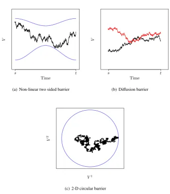
characterisa-tion of an entire sample path. . . 6

(a) Non-linear two sided barrier . . . 6

(b) Di↵usion barrier . . . 6

(c) 2-D circular barrier . . . 6

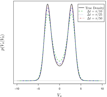
1.0.2 Density ofV⇡ and approximations given by an Euler discretisation with various mesh sizes, givenV0=0 where dVt=sin(Vt) dt+dWt. . . 7

1.1.1 Schematic diagram of thesis structure. . . 9

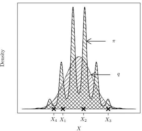
2.1.1 An illustration of the simulation ofX ⇠⇡by means of Inversion Sampling. 17 2.2.1 An illustration of a density composed of three weighted Normal densities. 19 2.4.1 An illustration of the simulation ofX ⇠⇡by means of Rejection Sampling. 21 2.5.1 An illustration of the simulation ofX ⇠ ⇡by means of Self-Normalised Importance Sampling. . . 25

(a) Graph of the proposal densityqalong with independent random samplesX1, . . . ,X4⇠q, overlaid with the target density⇡. . . 25

(b) Graph of ⇡ q for the assignment of weights for the drawn samples X1, . . . ,X4. The size of the vertical bar associated with each sam-ple represents its relative weight. . . 25

(18)

(a) An illustration of the unknown probability p, overlaid with the

graph composed of the estimate of pformed with the inclusion

of the firstkterms of the alternating Cauchy sequence. . . 30

(b) Case i)u> p. . . 30

(c) Case ii)u< p. . . 30

2.7.2 An illustration of the unbiased simulation of an event of unknown

prob-ability p, which can be represented as the limit of a sequence, by means

of Retrospective Bernoulli Sampling. . . 31

(a) An illustration of the unknown probability p, overlaid with the

graph composed of the estimate of pformed with the inclusion

of the firstkterms of an alternating sequence. Upon the inclusion

of the first ˆk terms the sequence becomes an alternating Cauchy

sequence. . . 31

(b) Case i)u> p. . . 31

(c) Case ii)u< p. . . 31

2.8.1 An illustration of Brownian motion and Brownian bridge sample path trajectories simulated on a fine mesh. . . 35

(a) Brownian motion sample path trajectories,W⇠ 0

0,1. . . 35

(b) Brownian bridge sample path trajectories,W ⇠ 0,00,1 . . . 35

2.8.2 An illustration of the minimum of 5,000 Brownian bridge sample path trajectories, and the maximum of 5,000 Brownian bridge sample path trajectories. . . 38

(a) Minimum or maximum without restriction. . . 38

(b) Minimum with restriction, W⇠ 0,10,0 ( ˆm2[ 1.25, 0.75]), or

maximum with restriction,W ⇠ 0,10,0 ( ˇm2[0.5,1.5]). . . 38 2.8.3 An illustration of Bessel bridge sample path trajectories,W ⇠ 0,00,1 (⌧,mˆ)

where⌧=0.5 and ˆm= 1, simulated on a fine mesh. . . 40

2.9.1 An illustration of a sample path of a time homogeneous Poisson process

with intensity =1 over the interval [0,5], where each asterisk indicates

an event time. . . 42 2.9.2 An illustration of a sample path of a time inhomogeneous Poisson

pro-cess with intensity (t) = |sin(t)| over the interval [0,5]. Each aster-isk indicates an event simulated under the dominating time homogeneous Poisson process, with those in green denoting the accepted events arising under the target Poisson process. . . 45

(19)

2.9.3 An illustration of sample paths of a compound Poisson process with in-tensity (t) =|cos (J(t))|and jump sizesµ(t)_⇠N( J(t )/2,⇡), over the

interval [0,5]. The colour of each asterisk corresponds to the jump times

of the similarly coloured compound Poisson process sample path. . . 48

3.1.1 Directed acyclic graph representing the latent and observation processes of a Hidden Markov Model. . . 52 3.1.2 An illustrative example of the Kalman filter applied to the HMM filtering

problem with SSDs as follows,X0⇠N(0,10),Xt|(Xt 1= xt 1)⇠N(0,1) andYt|(Xt = xt)⇠N(0,7.5). . . 60

(a) The observation process and Kalman filter with confidence

inter-val, overlaid with the underlying latent process. . . 60

(b) Trace of the process variances over time (the latent and

obser-vation process being conditional variances, whereas the Kalman filter being the marginal variance). . . 60 3.3.1 An illustrative example of a particle filter (with an optimal marginal

im-portance function selection) of 100 particles applied to the HMM filtering problem with SSDs as follows,X0⇠N(0,10),Xt|(Xt 1= xt 1)⇠N(0,1) andYt|(Xt = xt)⇠N(0,7.5). . . 69

(a) The observation process, particle filter and Kalman filter with

confidence interval, overlaid with the underlying latent process. . 69

(b) Trace of the process variances over time (the latent and

obser-vation process being conditional variances, whereas the particle filter is the posterior variance estimate). . . 69 3.3.2 An illustrative example of a particle filter (with a linearised optimal marginal

importance function selection) of 1000 particles applied to a highly

non-linear HMM filtering problem with SSDs as follows, X0 ⇠ N 0.05+

2.5/(1+ 0.12) + 8,p10 , Xt|(Xt 1 = xt 1) ⇠ N 0.5xt 1 + 2xt 1/(1+

x2

t 1)+8 cos(1.2(t 1)), p

10 andYt|(Xt = xt)⇠N⇣x2t/20, p1 ⌘

. . . 72

(a) The observation process and particle filter, overlaid with the

un-derlying latent process. . . 72

(b) A heat map of the empirical marginal filtering density over time

(20)

3.4.1 Directed acyclic graph representing the observation process of a Hidden

Markov Model and theith_{particle process under the SIS algorithm. . . 74}

3.4.2 An illustration of 250 particle sample paths arising from the Sequential

Importance Sampling/ Resampling algorithm under the SSDs in Figure

3.3.1 over the interval [1,30] using the optimal marginal importance

func-tion and multinomial resampling (see Secfunc-tion 3.5.1). Sample paths in black denote the ancestry of the particles constituting the empirical joint filtering density at time 30, whereas sample paths in red indicate those which were no longer included after a resampling point. . . 78 3.5.1 An illustration of Systematic Resampling. . . 82

(a) Partitioning of the CDF. . . 82

(b) Resampling of one sample from each partition of the CDF at

equidistant intervals. . . 82 3.5.2 An illustration of Stratified Resampling. . . 83

(a) Partitioning of the CDF. . . 83

(b) Resampling of one sample uniformly from each partition of the

CDF. . . 83 3.5.3 An illustration of Residual Resampling, where each vertical black line

represents the location of a particle and its associated weight. . . 84

(a) Before Residual Resampling. . . 84

(b) After the completion of the deterministic step in Residual

Resam-pling (Algorithm 3.5.4 Step 3). . . 84 3.6.1 “Bearings-Only Tracking” example of Gordon et al. [1993] – An

illus-trative example of an auxiliary particle filter of 2000 particles in which we wish to track a four dimensional target xt = (zx,z¯x,zy,z¯y)T which

moves on the x-y plane (where (zx,zy) denotes the targets position and

( ¯zx,z¯y) denotes the targets velocity) according to the following HMM

SSDs, X0 ⇠ MVN(m0,M0), Xt|(Xt 1 = xt 1) ⇠ MVN( xt 1, Vt) and

Yt|(Xt = xt) ⇠ N(tan 1(zy/zx),Wt) (where m0,M0, , ,V and W are parameterised as in Gordon et al. [1993]). . . 90

(a) Observation process and particle filter, overlaid with the

underly-ing latent process. . . 90

(b) Absolute distance between the particle filter estimate and the

un-derlying latent process over time. . . 90

(21)

4.2.1 Density ofV⇡ and approximations given by an Euler discretisation with

various mesh sizes, givenV0=0 where dVt=sin(Vt) dt+dWt. . . 109

4.2.2 Examples of test functions in which evaluation requires the characterisa-tion of an entire sample path. . . 110

(a) Non-linear two sided barrier . . . 110

(b) Di↵usion barrier . . . 110

(c) 2-D circular barrier . . . 110

5.1.1 Illustrative sample path skeleton output from the Unbounded Exact Algo-rithm (UEA; AlgoAlgo-rithm 5.1.3),SUEA(X)={(⇠i,X⇠i)i=+01,R}, overlaid with example sample path trajectoriesXrem _⇠ ⇣_⌦+1 i=1 X⇠_i ₁,X⇠_i ⇠i 1,⇠i ⌘ R. Hatched regions indicate layer information, whereas the asterisks indicate skeletal points. . . 124

(a) Example sample path skeletonSUEA(X), overlaid with example sample path trajectories. . . 124

(b) mapping of example sample path skeleton SUEA(X), and ex-ample sex-ample path trajectories. . . 124

5.1.2 Example trajectory of (X) whereX⇠ 0,x,yT R(X). . . 126

5.1.3 AUEA applied to the trajectory of (X) in Figure 5.1.2 (where X ⇠ x,y 0,T R(X)). . . 130

(a) After preliminary acceptance (Algorithm 5.1.4 Step 3) . . . 130

(b) After simulating⇠1(Algorithm 5.1.4 Step 4) . . . 130

(c) After simulating⇠2 . . . 130

(d) After simulating⇠3 . . . 130

5.1.4 Illustrative sample path skeleton output from the Adaptive Unbounded Exact Algorithm (AUEA; Algorithm 5.1.4), SAUEA(X) := n⇣⇠i,X⇠_i⌘+1 i=0, ⇣ R[⇠i 1,⇠i] X ⌘+1 i=1 o , overlaid with example sample path trajectories Xrem _⇠ ⇣ ⌦+1 i=1 X⇠_i ₁,X⇠_i ⇠i 1,⇠i R [⇠i 1,⇠i] X ⌘ . Hatched regions indicate layer information, whereas the asterisks indicate skeletal points. . . 132

(a) Example sample path skeletonSAUEA(X), overlaid with example sample path trajectories. . . 132

(22)

5.2.1 Illustrative sample path skeleton output from the Conditioned Unbounded Exact Algorithm (CUEA; Algorithm 5.2.1),SCUEA(X)=n⇣⇠i,X⇠_i⌘+1

i=0,R o

, overlaid with example sample path trajectoriesXrem_⇠⇣_⌦+1

i=1

X⇠_i ₁,X⇠_i

⇠i 1,⇠i

⌘

R. Hatched regions indicate layer information, whereas the asterisks indicate skeletal points. . . 136

(a) Example sample path skeletonSCUEA(X), overlaid with example

sample path trajectories. . . 136

(b) mapping of example sample path skeletonSCUEA(X), and

ex-ample sex-ample path trajectories. . . 136 5.2.2 Illustrative sample path skeleton output from the Conditioned Adaptive

Unbounded Exact Algorithm (CAUEA; Algorithm 5.2.2),SCAUEA(X)=

n⇣ ⇠i,X⇠i

⌘+1

i=0,

⇣

R[⇠i 1,⇠i] X

⌘+1

i=1

o

, overlaid with example sample path trajectories

Xrem _⇠ ⇣_⌦+1 i=1

X⇠_i ₁,X⇠_i

⇠i 1,⇠i R [⇠i 1,⇠i] X

⌘

. Hatched regions indicate layer infor-mation, whereas the asterisks indicate skeletal points. . . 137

(a) Example sample path skeletonSCAUEA(X), overlaid with

exam-ple samexam-ple path trajectories. . . 137

(b) mapping of example sample path skeletonSCAUEA(X), and

ex-ample sex-ample path trajectories. . . 137 5.3.1 Illustrative sample path skeleton output from the Unbounded Exact

Algo-rithm (UEA; AlgoAlgo-rithm 5.1.3) incorporated within the Bounded Jump

Ex-act Algorithm (BJEA; Algorithm 5.3.1),SBJEA(X)=SN

⇤

T+1 j=1

n⇣ ⇠_ij,X_⇠j

i

⌘j+1

i=0 ,

R[ j 1, j] X

o

, overlaid with example sample path trajectoriesXrem_⇠ x,y

0,T SBJEA.

Hatched regions indicate layer information, whereas the asterisks indicate skeletal points. . . 141

(a) Example sample path skeletonSBJEA(X), overlaid with example

sample path trajectories. . . 141

(b) mapping of example sample path skeletonSBJEA(X), and

ex-ample sex-ample path trajectories. . . 141 5.3.2 Illustrative sample path skeleton output from the Adaptive Unbounded

Jump Exact Algorithm (AUJEA; Algorithm 5.3.3),SAUJEA(X) :=SN_j₌T₁+1

S[ j 1, j)

AUEA (X), overlaid with example sample path trajectoriesXrem⇠

⇣ ⌦m+1

i=1

X_i ₁,X_i

i 1, i R

[ i 1, i] X

⌘

. Hatched regions indicate layer information, whereas the asterisks indicate skeletal points. . . 146

(23)

(a) Example sample path skeletonSAUJEA(X), overlaid with exam-ple samexam-ple path trajectories. . . 146

(b) mapping of example sample path skeletonSAUJEA(X), and

ex-ample sex-ample path trajectories. . . 146 5.4.1 Illustrative sample path skeleton output from the Conditioned Unbounded

Jump Exact Algorithm (CUJEA; Algorithm 5.4.1),SCUJEA(X) :=S_iN₌T₁+1 n⇣

⇠i,j,X⇠i,j

⌘(i)+1

j=0 ,RX[ i 1, i] o

, overlaid with example sample path

trajecto-ries Xrem _⇠ ⇣_⌦NT+1

i=1 ⇣

⌦i+1

j=1

X⇠_i,_j ₁,X⇠_i,_j

⇠i,j 1,⇠i,j

⌘

Ri⌘. Hatched regions indicate

layer information, whereas the asterisks indicate skeletal points. . . 158

(a) Example sample path skeletonSCUJEA(X), overlaid with

(b) mapping of example sample path skeletonSCUJEA(X), and

ex-ample sex-ample path trajectories. . . 158 5.4.2 Illustrative sample path skeleton output from the Conditioned Adaptive

Unbounded Jump Exact Algorithm (CAUJEA; Algorithm 5.4.2),SCAUJEA(X)

:= S_iN₌T₁+1n⇣⇠i,j,X⇠i,j

⌘(i)+1

j=0 , ⇣

R[⇠i,j 1,⇠i,j] X[ i 1, i]

⌘(i)+1

j=1 o

, overlaid with example

sam-ple path trajectoriesXrem_⇠⇣_⌦NT+1 i=1

⇣ ⌦i+1

j=1

X⇠_i,_j ₁,X⇠_i,_j

⇠i,j 1,⇠i,j R [⇠i,j 1,⇠i,j] i

⌘⌘

. Hatched regions indicate layer information, whereas the asterisks indicate skeletal points. . . 159

(a) Example sample path skeletonSCAUJEA(X), overlaid with

(b) mapping of example sample path skeleton SCAUJEA(X), and

example sample path trajectories. . . 159

6.1.1 An illustration of the reflection of a Brownian motion sample path around a boundary. . . 163

6.1.2 Example sample path trajectoriesW⇠ xs,,ty (W 2[`, ]). . . 165

6.1.3 Example sample path trajectories

W ⇠ sx,,ty Wu 2 ⇥x+ (y x) ·(u s)/(t s)+ `,x+ (y x)· (u

s)/(t s)+ ⇤,₈u₂[s,t] . . . 168 6.1.4 Example sample path trajectoriesW⇠ xs,,ty (X⌧=mˆ,mˇ 2[(x_y), ]). . 169

6.1.5 Example sample path trajectories

W ⇠ sx,,ty ( ˆm2[`#,`"],mˇ 2[ #, "],q1:n,W). . . 180

(24)

(b) n=3 . . . 180

6.1.6 Example sample path trajectoriesW⇠ xs,,ty (L,U,q1:n,W). . . 183

(a) n=0 . . . 183

(b) n=4 . . . 183

6.3.1 Density of intersection layer intermediate point overlaid with piecewise constant bound calculated using a mesh of size 20 over the interval [`_#, _"] and the corresponding local Lipschitz constants. . . 200 6.3.2 Illustration of 9 possible (disjoint) bisections. . . 203 6.3.3 Illustration of 4 possible refinements. . . 206

7.0.1 Directed acyclic graph representing the latent and observation processes of a Hidden Markov Model. . . 209 7.2.1 An illustrative example of an Exact Propagation Particle Filter (EPPF;

Algorithm 7.2.1) and a Bounded Random Weight Particle Filter (BRWPF; Algorithm 7.2.2) of 2,000 particles applied to the HMM filtering problem

with SSDs as follows, X0 ⇠ N(0,5),Yt|(Xt = xt) ⇠ N(0,10) and the

latent process is governed by a jump di↵usion with the following SDE,

dXt = sin(Xt-) dt+ dWt + dJ_T,⌫ where (Xt) = cos2(Xt) and f⌫(Xt) =

N(sin(Xt),1). In subfigures (b) and (c) we show for this example the

ancestral paths of the particles. Paths in black denote ancestral paths of the particles comprising the empirical filtering density at time 100, whereas those in other colours indicate that they are no longer included after some resampling point. . . 224

(a) The observation process, EPPF and BRWPF, overlaid with the

underlying latent process. . . 224

(b) EPPF particle ancestral paths. . . 224

(c) BRWPF particle ancestral paths. . . 224

8.1.1 Illustration of standard✏-strong simulation of a jump di↵usion sample

path, overlaid with sample path. . . 230

(a) Sample path skeleton . . . 230

(b) Aftern=2 bisections . . . 230

(c) Aftern=4 bisections . . . 230

(d) Aftern=6 bisections . . . 230

(e) Aftern=8 bisections . . . 230

(f) Aftern=10 bisections . . . 230

(25)

8.1.2 Illustration of modified tolerance based ✏-strong simulation of a jump

di↵usion sample path, overlaid with sample path. . . 231

(a) Sample path skeleton . . . 231

(b) X" _X# _₀_._{5 . . . 231}

(c) X" _X# _₀_._{4 . . . 231}

(d) X" _X# _₀_._{3 . . . 231}

(e) X" _X# _₀_._{2 . . . 231}

(f) X" _X# _₀_._{1 . . . 231}

8.3.1 Illustration of the determination of whether a 2-sided non-linear barrier has been crossed by a sample path using a finite dimensional sample path skeleton, overlaid with an illustration of the underlying sample path. . . . 238

(a) No barrier crossing . . . 238

(b) Barrier crossed . . . 238

8.3.2 Nonlinear two sided barrier example: Summary figures computed using 100000 sample paths. . . 239

(a) Kernel density estimates of the transition densities of subsets of

sample paths simulated from the measure induced by (8.14). . . . 239

(b) Empirical CDF of barrier crossing probability by time (crossing

time evaluated within interval of length ✏ _ 10 4). Upper and

lower black lines indicate upper and lower bounds for the empir-ical CDF, whereas the red dotted line indicates the average of the two bounds. . . 239

8.3.3 Illustration of the determination of whether two di↵usion sample paths

cross one another using finite dimensional sample path skeletons, overlaid with an illustration of the underlying sample paths. . . 242

(a) No crossing . . . 242

(b) Crossing . . . 242

8.3.4 Jump di↵usion crossing example: Summary figures computed using 100000

sample paths. . . 243

(a) Kernel density estimates of the transition densities of subsets of

(26)

(b) Empirical CDF of jump di↵usion crossing probability (crossing

time evaluated within interval of length ✏ _ 10 4). Upper and

lower black lines indicate upper and lower bounds for the empir-ical CDF, whereas the red dotted line indicates the average of the two bounds. . . 243 8.3.5 Illustration of the determination of whether a 2-D sample path crosses a

circular barrier using a finite dimensional sample path skeleton. Inscribed rectangles denote regions where for some time interval sample paths are constrained. Black and infilled red rectangles denote intervals constrained entirely within or out-with the circle respectively. Dotted black and red rectangles denote intervals with undetermined or partial crossing respec-tively. . . 245

(a) No barrier crossing . . . 245

(b) Barrier crossed . . . 245

8.3.6 2-D jump di↵usion with circular barrier example: Figures computed

us-ing 50000 sample paths. . . 246

(a) Contour plot of kernel density estimate of killed di↵usion

transi-tion density with circular barrier of radius 1.6. . . 246

(b) Empirical probabilities of crossing centred circles of increasing

radius (indicated by crosses) using a common collection of sam-ple paths, overlaid with 95% Clopper-Pearson confidence inter-vals (indicated by blue bar). . . 246

8.3.7 2-D jump di↵usion with circular barrier example: Exit point figures

(com-puted using a common collection of 50000 sample paths). . . 247

(a) Circle of radius 1.6 exit angle by exit time (crossing time and exit

angle evaluated within intervals of length✏ _ 10 3_and_✓ _₁₀ 3

respectively). . . 247

(b) Circle exit time by circle radius (crossing time evaluated within

interval of length✏ _10 3_{). . . 247}

B.0.1 Illustration of 9 possible (disjoint) bisections. . . 255

(27)

List of Tables

8.1 Nonlinear two sided barrier example: Barrier crossing probabilities (com-puted using 100000 sample paths). . . 237

8.2 Jump di↵usion crossing example: Crossing probabilities (computed using

(28)

1

Introduction

“I’m going for fearsome here, but I just don’t feel it! I think I’m just coming o↵as annoying.”

—Rex, Toy Story

Di↵usions and jump di↵usions are widely used across a number of application areas. An

extensive literature exists in economics and finance, spanning from the seminal Black-Scholes model (see for instance, Black and Black-Scholes [1973] and Merton [1973, 1976])

to the present (for instance, Eraker et al. [2003] and Barndor↵-Nielsen and Shephard

[2004]). Other applications can be easily found within both the physical sciences (Pic-chini et al. [2009]) and life sciences (Golightly and Wilkinson [2006, 2008]) to name but

a few. A jump di↵usionV : ! is a Markov process, which in this thesis we define to

be the solution to a stochastic di↵erential equation (SDE) of the following form (denoting

Vt :=lims"tVs),

dVt = (Vt-) dt+ (Vt-) dWt+ dJt,µ, V0=v2 , t2[0,T], (1.1)

where : ! and : ! + denote the (instantaneous) drift and di↵usion

co-efficients respectively,Wt is a standard Brownian Motion andJt,µ denotes a compound

Poisson process. J ,µ

t is parameterised with (finite) jump intensity : ! +and jump

size coefficientµ : _! with jumps distributed with density fµ. All coefficients are

themselves (typically) dependent on Vt. Regularity conditions are assumed to hold to

ensure the existence of a unique non-explosive weak solution (see for instance [Øksendal and Sulem, 2004, Chap. 1] and [Platen and Bruti-Liberati, 2010, Chap. 1.9]). To ap-ply the methodology developed within this thesis we primarily restrict our attention to

univariate di↵usions and require a number of additional conditions on the coefficients of

(1.1), details and a discussion of which can be found in Section 1.3.

(29)

Motivated by the wide range of possible applications we are typically interested in

(di-rectly or indi(di-rectly) the measure ofVon the path space induced by (1.1), denoted v_{. As}

v_{is typically not explicitly known then in order to compute expected values} _v_[_h₍_V_)],

for various test functionsh, we can construct a Monte Carlo estimator. In particular, if it is possible to draw independentlyV(1)_,_V(2)_{, . . . ,}_V(N) _⇠ v _{then by applying the strong law}

of large numbers we can construct a consistent estimator of the expectation (unbiasedness following directly by linearity),

w.p. 1: lim

N!1

1

N

n X

i=1

h(V(i))= v[h(V)]. (1.2)

Unfortunately, as di↵usion sample paths are infinite dimensional random variables it isn’t

possible to draw an entire sample path from v_{– at best we can hope to simulate some}

fi-nite dimensional subset of the sample path, denotedVfin_{(we further denote the remainder}

of the sample path byVrem_:₌_V_\_Vfin_{). Careful consideration has to be taken as to how to}

simulateVfin_{as any numerical approximation impacts the unbiasedness and convergence}

of the resulting Monte Carlo estimator (1.2). Equally, consideration has to be given to the form of the test functionh, to ensure it’s possible to evaluate it givenVfin_.

To illustrate this point we consider some possible applications. In Figures 1.0.1(a),

1.0.1(b) and 1.0.1(c) we are interested in whether a simulated sample path V ⇠ v,

crosses some barrier (i.e. for some setAwe haveh := (V 2 A)). Note that in all three

cases in order to evaluatehwe would require some characterisation of the entire sample

path (or some further approximation) and even for di↵usions with constant coefficients

and simple barriers this is difficult. For instance, as illustrated in Figure 1.0.1(c), even in

the case where v _{is known (for instance when} v_{is Wiener measure) and the barrier is}

known in advance and has a simplistic form, there may still not exist any exact approach to evaluate barrier crossing.

Di↵usion sample paths can be simulated approximately at a finite collection of time points

bydiscretisation (see for instance Jacod and Protter [2012], Kloeden and Platen [1992] and Platen and Bruti-Liberati [2010] for an extensive account of such methods), noting that as Brownian motion has a Gaussian transition density then over short intervals the

transition density of (1.1) can be approximated by one with fixed coefficients (by a

(30)

simulated over into a fine mesh (for instance, of size t), then iteratively (at each mesh

point) fixing the coefficients and simulating the sample path to the next mesh point.

It is hoped the simulated sample path (generated approximately at a finite collection of

mesh points) can be used as a proxy for an entire sample path drawn exactly from v_.

More complex discretisation schemes exist, but all su↵er from common problems. In

particular, minimising the approximation error (by increasing the mesh density) comes at the expense of increased computational cost, and further approximation or interpola-tion is needed to obtain the sample path at non-mesh points (which can be non-trivial).

As illustrated in Figure 1.0.2, even when our test functionh only requires the

simula-tion of sample paths at a single time point, discretisasimula-tion introduces approximasimula-tion error

resulting in the loss of unbiasedness of our Monte Carlo estimator (1.2). If v _{has a}

highly non-linear drift, or includes a compound Poisson process, orhrequires simulation

of sample paths at a collection of time points, then this problem is exacerbated. In the

case of the examples in Figure 1.0.1, mesh based discretisation schemes don’t sufficiently

characterise simulated sample paths for the evaluation ofh.

Recently, a new class ofExact Algorithms for simulating sample paths at finite

collec-tions of time points without approximation error have been developed for both di↵usions

[Beskos and Roberts, 2005; Beskos et al., 2006a, 2008; Chen and Huang] and jump dif-fusions [Casella and Roberts, 2010; Giesecke and Smelov, Forthcoming; Gonc¸alves and Roberts, 2013]. These algorithms are based on rejection sampling, noting that sample

paths can be drawn from the (target) measure v _{by instead drawing sample paths from}

an equivalent proposal measure v_{, and accepting or rejecting them with probability}

pro-portional to the Radon-Nikod´ym derivative of v _{with respect to} v_{. However, as with}

discretisation schemes, given a simulated sample path at a finite collection of time points subsequent simulation of the sample path at any other intermediate point may require ap-proximation or interpolation and may not be exact. Furthermore, we are again unable to evaluate test functions of the type illustrated in Figure 1.0.1.

The key contribution of this thesis is the introduction of a novel mathematical framework for constructing exact algorithms which addresses this problem. In particular, instead of exactly simulating sample paths at finite collections of time points, we focus on the

extended notion of simulatingskeletonswhich in addition characterise the entire sample

path.

(31)

Definition 1(Skeleton). A skeleton (S) is a finite dimensional representation of a di↵u-sion sample path (V ⇠ v), that can be simulated without any approximation error by means of a proposal sample path drawn from an equivalent proposal measure ( v_{) and accepted with probability proportional to} d v

d v, which is sufficient to restore

the sample path at any finite collection of time points exactly with finite computation where V|S ⇠ v|S. A skeleton typically comprises information regarding the sample path at a finite collection of time points and path space information which ensures the sample path is almost surely constrained to some compact interval.

Methodology for simulating skeletons (the size and structure of which is dependent on exogenous randomness) is driven by both computational and mathematical considerations (i.e. we need to ensure the required computation is finite and the skeleton is exact).

Central to both notions is that the path space of the proposal measure v_{can be partitioned}

(into a set of layers), and that the layer to which any sample path belongs to can be

simulated.

Definition 2 (Layer). A layer R(V), is a function of a di↵usion sample path V ⇠ v

which determines the compact interval to which any particular sample path V(!) is constrained.

To illustrate the concept of a layer and skeleton, we could for instance haveR(V)=inf{i2

:8u2[0,T],Vu2[v i,v+i]}andS={V0 =v,VT =w,R(V)=1}.

We show that a valid exact algorithm can be constructed if it is possible to partition the proposal path space into layers, simulate unbiasedly to which layer a proposal sample path belongs and then, conditional on that layer, simulate a skeleton. Our exact algorithm framework for simulating skeletons is based on three principles for choosing a proposal measure and simulating a path space layer,

Principle 1(Layer Construction). The path space of the process of interest, can be par-titioned and the layer to which a proposal sample path belongs can be unbiasedly simulated, R(V)⇠R:= v R 1.

Principle 2(Proposal Exactness). Conditional on V0 =v, VT and R(V), we can simulate

any finite collection of intermediate points of the trajectory of the proposal di↵usion exactly, V ⇠ v|R 1₍_R₍_V₎₎.

(32)

with the following additional principle.

Principle 3 (Path Restoration). Any finite collection of intermediate (inference) points, conditional on the skeleton, can be simulated exactly, Vt1, . . . ,Vtn ⇠ v|S.

In developing a methodological framework for simulating exact skeletons of di↵usion

sample paths we make several additional contributions. We make a number of method-ological improvements to existing exact algorithms with potential for substantial com-putational benefit and extension of the applicability of existing algorithms. In addition,

we introduce a novel class ofadaptive exact algorithmsfor di↵usions, di↵usion bridges,

jump di↵usions and jump di↵usion bridges, underpinned by new results for simulating

Brownian path space probabilities (which are of separate interest) andlayered Brownian

motion(Brownian motion conditioned to remain in a layer).

By application of the results developed in this thesis we present methodology for

par-ticle filtering for partially observed (jump) di↵usions. Furthermore, we present a

signifi-cant extension to✏-Strong Simulationmethodology (recently introduced by Beskos et al.

[2012], and allowing the simulation of upper and lower bounding processes which almost surely constrain stochastic process sample paths to any specified tolerance), from

Brown-ian motion sample paths to a general class of jump di↵usions, and introduce novel results

to ensure the exactness of the methodology.

Finally, we highlight a number of possible applications of the methodology developed in this thesis by returning to the examples introduced in Figure 1.0.1. We demonstrate that it is possible not only to simulate skeletons exactly from the correct target measure but also to evaluate exactly whether or not non-trivial barriers have been crossed and so construct Monte Carlo estimators for computing barrier crossing probabilities. It should be noted that there are a wide range of other possible direct applications of the method-ology in this thesis, for instance, the evaluation of path space integrals and barrier hitting times to arbitrary precision, among many others.

The remainder of this introductory chapter is structured as follows: In Section 1.1 we detail the structure of this thesis and how the content of the chapters relate to one another. In Section 1.2 we provide a summary of the key contributions of this thesis. Finally, in Section 1.3 we briefly discuss the recurrent conditions required to implement the method-ology developed in this thesis.

(33)

Time

V

s t

(a) Non-linear two sided barrier

Time

V

s t

(b) Di↵usion barrier

V1

V

2

[image:33.595.144.487.187.579.2]

(c) 2-D circular barrier

(34)

−10 −5 0 5 10

V⇡

p

(

V⇡

|

V0

)

[image:34.595.200.429.282.489.2]

True Density t=⇡/10 t=⇡/25 t=⇡/50

Figure 1.0.2: Density of V⇡ and approximations given by an Euler discretisation with

various mesh sizes, givenV0=0 where dVt=sin(Vt) dt+dWt.

(35)

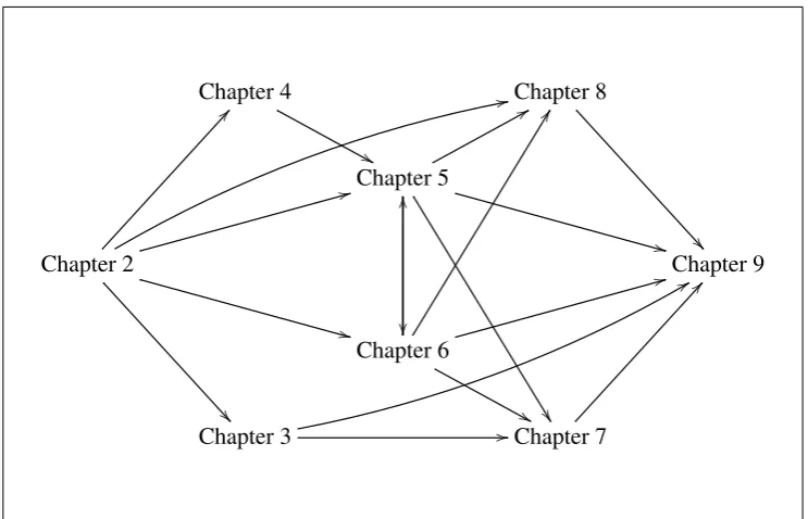
1.1 Thesis Structure

In Figure 1.1.1 we present a schematic diagram of how the content of each of the chapters in this thesis relate to one another. This thesis is essentially broken into two key parts: Part I is primarily a review of relevant existing literature pertinent to this thesis; whereas in Part II we present our methodology (as discussed in the introductory remarks of this chapter and summarised in Section 1.2) within the context of existing literature.

Part I is comprised of Chapters 2, 3 and 4. In Chapter 2 we selectively review a number of elementary Monte Carlo methods employed within this thesis, including Monte Carlo methods for simulating finite dimensional sample path trajectories of Brownian motion and related stochastic processes, and Monte Carlo methods for simulating sample paths of Poisson processes. In Chapter 3 we motivate and present a review of sequential Monte Carlo methods. We conclude Part I of this thesis in Chapter 4, where we provide an in-troductory level overview of elements of stochastic calculus required in this thesis and

briefly review existing discretisation methods for simulating di↵usion sample paths.

Part II is comprised of Chapters 5, 6, 7 and 8. In Chapter 5 we present a novel

math-ematical framework for simulating (jump) di↵usion and (jump) di↵usion bridge sample

path skeletons without approximation error (exact algorithms). In Chapter 6 we present new results for simulating quantities related to various Brownian bridge path space con-structions, which together allow the simulation of layered Brownian bridge sample path skeletons, and hence the implementation of the exact algorithms in Chapter 5. In Chapter

7 we present methodology for particle filtering for partially observed (jump) di↵usions.

Finally, we conclude Part II of this thesis in Chapter 8 where we outline methodology for simulating upper and lower bounding processes which almost surely constrain (jump)

di↵usion and (jump) di↵usion bridge sample paths to any specified tolerance (✏-strong

simulation). We additionally demonstrate that our methodology can be applied to

deter-mine exactly whether a di↵usion or jump di↵usion sample path crosses various types of

non-trivial barrier.

(36)

Chapter 4

&&

Chapter 8

Chapter 5

✏✏

88

⇡⇡

++

Chapter 2

@@

33

++

22

Chapter 9

Chapter 6

OO

&&

EE

33

Chapter 3 //

88

Chapter 7

[image:36.595.132.504.105.344.2]

@@

Figure 1.1.1: Schematic diagram of thesis structure.

1.2 Thesis Contributions

In summary, the main contributions of this thesis are as follows:

– A mathematical framework for constructing exact algorithms, along with a new

class of adaptive exact algorithms, which allow both (jump) di↵usion and (jump)

di↵usion bridge sample path skeletons to be simulated without discretisation error

(see Chapter 5).

– An extension of existing exact algorithms to satisfy Principle 3 (see Chapter 5 and in particular Sections 5.1.1, 5.3.1, 5.4 and 6.2), including a number of general methodological improvements (see Chapters 5 and 6).

– Methodology for simulating unbiasedly events of probability corresponding to var-ious Brownian path space probabilities and simulating layered Brownian bridge sample path trajectories (see Chapter 6).

– An extension of methodology for particle filters to the setting in which the transition

density of the latent process is governed by a jump di↵usion (see Chapter 7).

(37)

– Methodology for the✏-strong simulation of (jump) di↵usion and (jump) di↵usion

bridge sample paths, along with a novel exact algorithm based on this construction (see Chapter 8).

– A new approach for constructing Monte Carlo estimators to compute irregular bar-rier crossing probabilities, simulating first hitting times to any specified tolerance

and simulating killed di↵usion sample path skeletons (see Section 8.3). This work

is presented along with examples based on the illustrations in Figure 1.0.1.

Throughout this thesis we make a number of additional minor contributions, which are pointed out in the relevant sections.

1.3 Thesis Conditions

Throughout this thesis a number of the methodological results and algorithms that we present share a common set of recurrent conditions. For convenience we briefly intro-duce these conditions and motivate their requirement in this section, referring back to them as necessary (a number of the methodological results and algorithms require ad-ditional conditions, however these are stated and motivated in the appropriate sections). The motivation for the conditions in this section is to establish a number of results (Re-sults 1–4) that we also summarise in this section, however these re(Re-sults are revisited as required and extended upon in later chapters.

To present our work in full generality we assume Conditions 1–5 hold (see below), how-ever, these conditions can be difficult to check and so in Section 1.3.1 we discuss verifiable

sufficient conditions under which Results 1–4 hold.

Condition 1(Solutions). The coefficients of (1.1) are sufficiently regular to ensure the existence of a unique, non-explosive, weak solution.

Condition 2(Continuity). The drift coefficient 2C1_{. The volatility coefficient} ₂_C2

and is strictly positive.

Condition 3(Growth Bound). We have that9K>0such that_| (x)_|2+|| (x)||2 K(1+

|x|2)8x2 .

(38)

Conditions 2 and 3 are sufficient to allow us to transform our SDE in (1.1) into one with

unit volatility (letting 1, . . . , N_T denote the jump times in the interval [0,T], 0 := 0

and NT+1 := NT+1 :=T, and denoting byVctsas the continuous component ofV),

Result 1(Lamperti Transform [Kloeden and Platen, 1992, Chap. 4.4]). Let⌘(Vt) =: Xt

be a transformed process, where⌘(Vt) := R_vV⇤t1/ (u) du (where v⇤ is an arbitrary

element in the state space of V). Denoting by Nt := Pi 1 { i  t}a Poisson jump

counting process (with respect toFtN) and applying Itˆo’s formula for jump di↵usions

to find dXt we have,

dXt = 

⌘0dV_tcts+⌘00⇣dV_tcts⌘2/2 +⇥⌘(Vt-+µ(Vt-)) ⌘(Vt-)⇤ dNt

= 2 66666 64

⇣

⌘ 1(Xt-)⌘

⌘ 1(Xt-)

0⇣_⌘ 1₍_X t-)⌘

2

3 77777 75 | {z }

↵(Xt-)

dt+ dWt+⇣⌘h⌘ 1(Xt-)+µ⇣⌘ 1(Xt-)⌘i Xt-⌘ dNt | {z }

dJ ,⌫ t

.

(1.3)

This transformation is typically possible for univariate di↵usions and for a significant

class of multivariate di↵usions (see for instance, A¨ıt-Sahalia [2008]). We revisit the

Lam-perti transform in Section 4.1.2, providing a more detailed account.

As a consequence of Result 1, in this thesis we frequently restrict our attention to SDEs

with unit volatility coefficient as in (1.3) without loss of generality. As such we introduce

the following simplifying notation. In particular, we denote by x

0,T the measure induced

by (1.3), by x

0,Tthe measure induced by the driftless version of (1.3),A(u) := Ru

0 ↵(y) dy and set (Xs) := ↵2(Xs)/2+↵0(Xs)/2. If = 0 in (1.3) then _0,x_T is Wiener measure.

Furthermore, we impose the following final condition,

Condition 5( ). There exists a constant > ₁such that _infs2[0,T] (Xs).

It is necessary within this thesis to establish that the Radon-Nikod´ym derivative of x

0,T

with respect to x

0,T exists (Result 2) and can be bounded on compact sets (Results 3

and 4) under Conditions 1–5. We provide a more detailed account of Result 2 and the

Radon-Nikod´ym derivative of x

0,T with respect to alternate measures in Section 4.1.3.

Result 2(Radon-Nikod´ym derivative [Øksendal and Sulem, 2004; Platen and Bruti-Liberati,

2010]). Under Conditions 1–4, the Radon-Nikod´ym derivative of x

0,T with respect

(39)

to x

0,T exists and is given by Girsanov’s formula.

d x

0,T

d x

0,T

(X)=exp (Z T

0 ↵(Xs) dWs 1 2

Z T

0 ↵

2₍_X s) ds

)

. (1.4)

As a consequence of Condition 2, we have A2C2_{and so we can apply Itˆo’s formula}

to remove the stochastic integral,

d x

0,T

d x

0,T

(X)=exp 8 >><

>>:A(XT) A(x) Z T

0 (Xs) ds NT

X

i=1 h

A(X i) A(X i )

i9_>>=

>>;. (1.5)

In the particular case where we have a di↵usion ( =0) then,

d x

0,T

d x

0,T

(X)=exp (

A(XT) A(x) Z T

0 (Xs) ds

)

. (1.6)

Result 3(Quadratic Growth). As a consequence of Condition 3 we have that A has a quadratic growth bound and so there exists some T0<1such that8T T0:

c(y;x,T) := Z

exp

(

A(y) (y x)2 2T

)

dy<₁. (1.7)

Throughout this thesis we rely on the fact that upon simulating a path space layer (see

Definition 2) then8s 2 [0,T] (Xs) is bounded, however this follows directly from the

following result,

Result 4(Local Boundedness). By Condition 2,↵and↵0are bounded on compact sets. In particular, suppose 9`, ₂ such that ₈ t ₂ [0,T], Xt(!) 2 [`, ] 9LX :=

L(X(!))₂ ,UX :=U(X(!))2 such that8t2[0,T], (Xt(!))2[LX,UX].

1.3.1 Verifiable Sufficient Conditions

As discussed in [Øksendal and Sulem, 2004, Thm. 1.19] and [Mao and Yuan, 2006,

Sec. 3.3], to ensure Condition 1 it is sufficient to assume that the coefficients of (1.1)

(40)

C1,C2 <1(recalling that fµis the density of the jump sizes),

| (x)|2+|| (x)||2+ Z

|fµ(x,z)|2 ( dz)C1(1+|x|2), ₈x₂ , (1.8)

| (x) (y)|2+|| (x) (y)||2+ Z

|fµ(x,z) fµ(y,z)|2 ( dz)C2(|x y|2), 8x,y2 . (1.9)

(1.8) and (1.9) together with Condition 2 are sufficient for the purposes of ensuring

Con-ditions 1, 3, 4 and 5 hold, but are not necessary. Although easy to verify, (1.8) and (1.9) are somewhat stronger than necessary for our purposes and so we impose Condition 1 instead.

It is of interest to note that if we have a di↵usion (i.e. in (1.1) we have = 0) then,

by application of the Mean Value Theorem, Condition 2 ensures and are locally Lips-chitz and so (1.1) admits a unique weak solution (see Øksendal [2007]) and so Condition 1 holds. In particular, in this setting Results 1–4 will hold under Conditions 2, 3 and 5.

(41)

Part I

(42)

2

Monte Carlo Methods

“If the only tool you have is a hammer, you tend to see every problem as a nail.”

—Abraham Maslow

In this chapter we review a number of elementary Monte Carlo methodswhich are of

particular relevance to the methodology developed in this thesis as outlined in Chapter 1 and explored later. A fuller account of the methods discussed in this chapter along with the broader literature and applications can be found in a number of texts (see for instance Robert and Casella [2004], Kloeden and Platen [1992] and Kingman [1992]).

Monte Carlo methods are a class of statistical algorithms which, by means of exploiting the comparatively recent introduction of cheap and powerful computing, use the simu-lation of random processes to draw inference on quantities of interest. To motivate this we consider expectations of the following form which may, or may not be, analytically

tractable (whereh is some test function, ⇡some probability density and X is a random

variable with law⇡),

⇡[h(X)] :=

Z

h(x)·⇡(x) dx. (2.1)

Employing the notion first proposed by Metropolis and Ulam [1949] (which we term

Na¨ıve Monte Carloand present in Algorithm 2.0.1), note that if we were to simply

sim-ulate large numbers of random samples1 _{from the density}_⇡ _{(and this were possible),}

1_{Random Number Generators}_{: In this thesis we assume that it is possible to simulate any number}

of independent uniform random variables (u1,u2, . . . ⇠ U[0,1]). Some care ensuring generated random

variables are truly random has to be taken (see for instance [Ripley, 1987, Chap. 1] and [Robert and Casella, 2004, Chap. 2]). Particular consideration of random number generators in the context of di↵usions can be

(43)

then these could be used to compute an estimate of the expectation in (2.1) (which we

term the Monte Carlo estimator). More precisely, if we were to draw independently

X1,X2, . . . ,XN ⇠ ⇡, then by applying theStrong Law of Large Numbers(SLLN) we can

construct a consistent estimator of the expectation (with unbiasedness following directly by linearity),

w.p. 1: lim

N!1

1

N

N X

i=1

h(Xi)= ⇡[h(X)]. (2.2)

Furthermore, provided ar⇡[h(X)] =: 2 < 1, it can be shown by the Central Limit

Theorem(CLT) that we have,

lim

N!1

p

N

2 66666

4 ⇡[h(X)] 1 N

n X

i=1

h(Xi) 3 77777

5 D= ⇠, where⇠ ⇠N(0, 2). (2.3)

The number of algorithms and applications which stem from this simple simulation

ap-proach is vast. The central difficulty in employing this approach in practice is being able

to simulate independent and identically distributed random variables from the density⇡.

Addressing this problem is the theme linking the various Monte Carlo methods we review in the remainder of this chapter.

Algorithm 2.0.1 Na¨ıve Monte Carlo Algorithm (N random samples) [Metropolis and Ulam, 1949].

1. Foriin 1 toNsimulateXi ⇠⇡.

2. Compute the Monte Carlo estimatorId(X) := 1

N

PN

i=1h(Xi).

2.1 Inversion Sampling

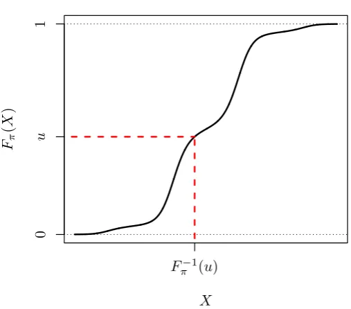
Inversion Sampling (see for example [Devroye, 1986, Part 3 Chap. 2]) is a method of

sampling from a density⇡, by inverting a randomly drawn uniform random variableu⇠

U[0,1]. Denoting F⇡ as the cumulative distribution function (CDF) of⇡, we define the

(44)

generalised inverse as follows,

F⇡1(u) :=inf_x {F⇡(x) u}. (2.4)

Noting that F⇡(x) 2 [0,1] 8x 2 , it is possible to draw from ⇡ by generating and

transforming a uniform random variableu ⇠ U[0,1] as illustrated in Figure 2.1.1 and

presented in Algorithm 2.1.1.

X F⇡

(

X

)

F 1

⇡ (u)

u

0

[image:44.595.184.438.273.496.2]

1

Figure 2.1.1: An illustration of the simulation ofX⇠⇡by means of Inversion Sampling.

Algorithm 2.1.1 Inversion Sampling Algorithm (N random samples) [Devroye, 1986, Part 3 Chap. 2].

1. Foriin 1 toNsimulateui ⇠U[0,1] and setXi =F_⇡1(ui).

(45)

This notion can be formalised by considering the following,

⇣

F⇡1(u)x

⌘

= (uF⇡(x))=F⇡(x)= (X x). (2.5)

It should be noted that this algorithm can be extended to draw in a computationally effi

-cient manner fromF⇡(x) conditional onx 2[`, ] (or similarly a percentile ofF⇡(x)) by modifying Algorithm 2.1.1 such thatui ⇠UhF⇡1(`),F⇡1( )

i

.

2.2 Composition Sampling

Suppose we wish to draw a random sample from a density formed through a weighted

composition of a number of other densities. In particular (denotingwj( 0) as the

con-tribution of the density⇡jto the composition such thatPni=1wi =1) suppose we have,

⇡= r X

j=1

wj⇡j, (2.6)

an example of which is illustrated in Figure 2.2.1.

As shown in [Ripley, 1987, Chap. 3.2] and as outlined in Algorithm 2.2.1, we can draw

a random sample from⇡by first sampling a contributing density⇡jwith probability

pro-portional to its weight (wj), then drawing from⇡j.

Algorithm 2.2.1Composition Sampling Algorithm (Nrandom samples) [Ripley, 1987].

1. Foriin 1 toNsample Ji ⇠categorical(w1, . . . ,wr) and sampleXi|(Ji= j)⇠⇡j.

2.3 Demarginalisation

Demarginalisationis a technique whereby artificial extension of a density (with the in-corporation of auxiliary variables) simplifies sampling from it. To illustrate this consider

the case where we want to draw a sample from ⇡(x), but this is not directly possible.

(46)

X

De

n

si

ty _w

1⇡1

w2⇡2

w3⇡3

⇡

Figure 2.2.1: An illustration of a density composed of three weighted Normal densities.

⇡(x_|y) is possible and⇡(x,y) admits⇡(x) as a marginal. In particular, we have,

⇡(x)= Z

Y⇡(x|y)·⇡(y) dy. (2.7)

We can sample from⇡(x) by first samplingY from⇡(y) and then sampling from⇡(x_|y).

This algorithm can be viewed as a black box to generate samples from ⇡(x) – Y can

be simply marginalised out (i.e. ‘thrown’ away). A fuller account of demarginalisation can be found in [Robert and Casella, 2004, Chap. 5.3], however it is worth noting that composition sampling (see Section 2.2) is an example of demarginalisation.