407 Knowledge of the genotype × environment (G × E)
interaction is important for the optimum use of particular genotypes in different production and breeding systems, especially for beef cattle which are kept in both intensive and extensive environ-ments. The adaptation of breeding systems in beef cattle was studied by Krupa et al. (2005) and Veselá et al. (2007). G × E interaction is defined as a change in the relative value of the performance of two or more genotypes in two or several different environ-ments. When comparing two different genotypes, the magnitude and statistical significance of this interaction is related mainly to the distinctness of genotypes or environment. In fact, such an inter-action is assumed to exist whenever two or more genotypes occur in two or several environments.
Two approaches are used to study G × E inter-action: either G × E interaction is included in the evaluated model or phenotype expression of the same trait in different environments is classified as two different production traits (Falconer, 1970). To apply these two approaches to the evaluation of G × E interaction, the environments should be divided into classes of a given environmental effect. The selection of a suitable approach to the clas-sification of G × E interaction was studied e.g. by Fernando (1984) and Mathur and Schlote (1995). A definition on the basis of a high number of levels with increasing values, i.e. reaction norm, may be another method (Kolmodin et al., 2002).
According to Lin and Togashi (2002), the defi-nitions of G × E interaction can be divided into
Supported by the Ministry of Education, Youth and Sports of the Czech Republic (Project No. MSM 6046070901) and by the Ministry of Agriculture of the Czech Republic (Project No. MZe 0002701401).
Selection of a suitable definition of environment for
the estimation of genotype × environment interaction
in the weaning weight of beef cattle
L. Vostrý
1,2, J. Přibyl
2, V. Jakubec
1, Z. Veselá
2, I. Majzlík
1 1Czech University of Life Sciences Prague, Prague, Czech Republic 2Institute of Animal Science, Prague-Uhříněves, Czech RepublicABSTRACT: Genotype by environment interactions for weaning weight in beef cattle were tested using several definitions of environments. Four breeds of beef cattle (Hereford, Aberdeen Angus, Beef Simmental, and Charolais) were represented. The environments were defined according to five criteria: altitude, produ-ction areas, economic value of the land, less favourable areas, and performance levels of a breed within herds. Ten mixed models were compared including the effects of direct and maternal genetics, herd-year-season, maternal permanent environmental, breed, environment, genotype × environment interaction, sex of calf, and age of dam. The suitability of the models was tested by Akaike’s Information Criterion, likelihood ratio test, and magnitude of the residual variance. The most suitable definitions of environment were less favoured areas and herd levels of performance. Estimates of direct heritability ranged from 0.07 to 0.19. Genotype × environment interactions should be included in a genetic evaluation model for interbreed comparisons of beef cattle in the Czech Republic.
Original Paper Czech J. Anim. Sci., 53, 2008 (10): 407–417
breed × environment interaction (between-breed interaction), which was investigated e.g. by Křížek et al. (1992), Brown et al. (1993) and Sandelin et al. (2002), and individual × environment interaction (within-breed interaction), which was studied e.g. by Notter et al. (1992), De Mattos et al. (2000).
Production characteristics of all beef cattle ani-mals are under routine ICAR recording across breeds in the Czech Republic. The objectives of this paper were to select a suitable definition of environment and to test the existence of G × E in-teraction for weaning weight at 210 days of age in beef cattle breeds under the conditions in the Czech Republic. Genotype was determined by the most frequent breeds of beef cattle, and five different definitions of environment were tested.
MATERIAL AND METHODS
G × E interaction was estimated for weaning weight at 210 days of age in the most frequent breeds of beef cattle kept in the Czech Republic during a period of 16 years (1990–2005).
The data were edited so that the components of variance between all the considered effects would be estimable (Vostrý et al., 2007). The data set in-cluded:
(1) Sires that had at least 5 offspring with tested performance.
(2) Herd × year × season (HYS) had at least 5 indi-viduals.
(3) Sires that had offspring in at least two HYS. (4) HYS which had progeny of at least two sires. (5) Mothers that had at least two offspring and at
least one half-sister.
The two most numerous breeds of medium body frame – Hereford (HE) and Aberdeen Angus (AA) – and the two most numerous breeds of large body frame – Beef Simmental (BS) and Charolais (CH) – were used for the estimation of G × E interaction. Each breed was represented by individuals with a gene proportion of 88 to 100% of the given breed. The total set consisted of 19 760 individuals.
Environments
Environment was classified according to these criteria:
(1) Economic value of agricultural lands (hereinaf-ter the economic value):
(a) low prices – average price maximally 1.5 Kč/ m;
(b) medium prices – average price from 1.5to 3.0 Kč/m;
(c) high prices – average price more than 3.0 Kč/m.
(2) Altitude:
(a) mountain – altitude above 600 m a.s.l.; (b) foothills – altitude from 450 to 600 m a.s.l.; (c) lowland – altitude up to 450 m a.s.l.. (3) Production areas:
(a) forage production – annual temperatures 5–6˚C, precipitation above 700 mm, steeply sloping and stony lands;
(b) cereal production – annual temperatures 5–8.5˚C, precipitation 550–700 mm; (c) sugar beet production – annual temperatures
8–9˚C, annual precipitation 500–650 mm. (4)Areas according to LFA: Categorisation of farm
land resources from the aspect of less favourable areas (LFA):
(a) mountain – above 600 m a.s.l. or 500 to 600 m a.s.l., with steeply sloping lands – in more than 50% of lands the gradient is higher than 7˚;
(b) barely cultivable land – low productivity of farm land, barely tillable soils and soils with reduced production potential;
(c) productive – with high productivity of farm land.
(5) Levels of performance of breeds achieved within a herd(hereinafter the herd level) (Kolmodin et al., 2002). Environment was divided into classes of herd levels according to average performance achieved in the particular HYS within breeds. HYS were ranked according to the average live weight achieved by breeds, and herd levels were composed so that about 33% HYS of the given breed would be in each level:
(a) high-level herd; (b) medium-level herd; (c) low-level herd.
The definition of environment and the testing of the existence of G × E interaction were performed by mixed models using the MIXED maximum likeli-hood procedure in the SAS statistical package (SAS, 2004) respecting Rasch and Mašata (2006):
Model 1
409 Model 2 corresponded to Model 1, but it did not
include the effect of interaction (Breed × Env)lm where:
yijklmo = weaning weight at 210 days of age
μ = general mean
Sexi = fixed effect of sex (either young bull or heifer)
FBj = fixed effect of litter size (either single or twin-born)
AgeMk = fixed effect of mother’s age Breedl = fixed effect of breed Envm = fixed effect of environment sirelo = random effect of sire within breed
hysmn = random effect of HYS within environ-ment
(Breed × Env)lm = interaction between breed (Breedl) and environment (Envm)
eijklmno = random error
The effects of HYS and sire were considered as random because of the high number of levels of these effects (HYS – 1 270 levels and sire – 602 levels).
Models 1 and 2 were used for the definition of a suitable environment only for further analysis. Therefore these models do not use relationships among sires, and no genetic variance is assumed.
The selection of a suitable definition of environ-ment was made on the basis of the number of sires with offspring in different environments related to the total number of sires (hereinafter the numbers of connecting sires), and the number of offspring of connecting sires related to the total number of individuals in the database, achieved values of re-sidual variance (σ2
e), and Akaike’s information
cri-terion (AIC). G × E interaction was tested on the basis of statistical significance of G × E interaction by a comparison of the values of residual variance and AIC between the model with G × E interaction
(Model 1) and the model without G × E interaction (Model 2). The ratio of connecting sires to their offspring in the entire database is crucial for testing the existence of G × E interaction.
The values of AIC were calculated from this equa-tion (Bozdogan, 2000):
AIC = –2logL(θ) + 2d
where:
logL(θ) = the logarithm of the value of likelihood function
d = the number of free parameters in the model Estimation of genetic parameters for the testing of genotype × environment interaction.
The estimation of genetic parameters was carried out using a single-trait animal model by the REML method. Definitions of environment for the estima-tion of genetic parameters and G × E interacestima-tion effect were based on a previous investigation.
Different models were tested (Table 1), based on the animal model used for the estimation of breeding value in the Czech Republic (Přibyl et al., 2003).
a σa2 σ
am
V
[
]
= A ⊗[
]
m σam σm2V(pe) = Iσ2
p e
V(HYS) = Iσ2 H YS
V(G × E) = Iσ2 G × E
V(e) = Iσ2
e
[image:3.595.62.536.589.690.2]The effects a and m are assumed to be correlated with each other, and the remaining effects are inde-pendent. The particular effects are also assumed to show normal random distribution with zero mean and variance (σ2):
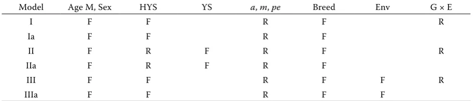
Table 1. Models
Model Age M, Sex HYS YS a, m, pe Breed Env G × E
I F F R F R
Ia F F R F
II F R F R F R
IIa F R F R F
III F F R F F R
IIIa F F R F F
Original Paper Czech J. Anim. Sci., 53, 2008 (10): 407–417
where: σ2
a
= additive genetic variance of direct effect σ2
m = additive genetic variance of maternal effect σam = genetic covariance of direct and maternal effect
(Cov(a, m)) σ2
p e = variance of the effect of permanent maternal envi-ronment
σ2
H YS = variance of HYS effect
σ2
G × E = variance of the effect of genotype × environment
interaction σ2
e
= variance of the effect of residual error
A = relationship matrix
I = identity matrix
The computation programme VCE 5.1 (Kovač et al., 2002) was used for the estimation of variance-covariance components and their mean errors. The following population parameters were derived from the estimated variance-covariance components: σ2
y = phenotype variance (σ2y = σ2a + σ2m + σam + σ2p e +
+ σ2
G × E + σ2e ) (Willham, 1979)
h2
a = coefficient of direct heritability (h2a = σ2a /σ2y )
h2
m = coefficient of maternal heritability (h2m = σ2m /σ2y )
c2 = the ratio of variance of permanent maternal environment to phenotype variance (c2 = σ2
p e/σ2y )
G × E2 = the ratio of variance of genotype × environ-ment interaction to phenotype variance (G × E2 = σ2
G × E/σ2y )
ram = genetic correlation of direct and maternal effect (ram = σam/(σa× σm))
The suitability of the model was tested by AIC and by the Likelihood Ratio test (LR, Kaps and Lamberson, 2004), which is based on a comparison of the values of the likelihood function of two models.
L(reduced)
χ2 = –2log –––––––––– = 2(–logL(reduced) + logL(full)) L(full)
where:
χ2 = the value of chi-squared test
L(reduced) = the value of the likelihood function of a reduced model – model without G × E effect
L(full) = the value of the likelihood function of a full model – model with G × E effect
RESULTS AND DISCUSSION Selection of a suitable definition of environment
[image:4.595.70.532.588.718.2]Table 2 shows that both Models (1 and 2) reached the same values of residual variance for all defini-tions of environment. The only exception was the definition according to herd level, which had lower values. Model 2 reached slightly higher values of residual variance. The highest suitability evalu-ated by AIC was the environment according to herd level and economic value. On the contrary, definitions according to altitude and LFA were the least suitable if the AIC value was used. The lower values of AIC and residual variance for Model 1 indicate the effect of G × E interaction. The va-lues of connecting sires and their offspring, similar to those of residual variance, did not demonstrate any marked differences between the environments. An exception was the definition according to herd level, when the values of connecting sires and their offspring reached twofold values compared to the other definitions of environment. These high values were caused by the creation of herd level classes.
Table 2. Significance of models evaluated according to the definitions of environment by means of a mixed model
Altitude Production areas Economic value LFA Herd level F < Pr <0.0001 <0.0001 <0.0001 <0.0001 <0.0001
Numbers of connecting sires 37% 37% 42% 37% 74%
Offspring of connecting sires 54% 47% 58% 54% 90%
σ2
e
– Model 1 958.25 958.54 957.29 957.68 954.12
σ2
e
– Model 2 958.72 958.64 958.47 958.75 954.51
AIC – Mode 1 195 091.20 195 035.50 195 030.60 195 102.40 193 343.50 AIC – Mode 2 195 157.60 195 181.60 195 105.40 195 166.00 193 393.10
F < Pr – statistical significance of the effect of genotype × environment interaction; σ2
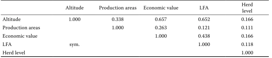
411 Table 3 shows the values of the correlation which
evaluates the overlapping of definitions of envi-ronment. By this correlation the identity of the inclusion of individuals in the particular areas ac-cording to different definitions of environment was evaluated. The highest values of correlation were estimated between definitions according to LFA, altitude (0.652), and economic value (0.438). A high correlation was also calculated between environ-mental definitions according to altitude and eco-nomic value (0.657). The consideration of altitude and the average price of land in LFA methodology caused the high values of correlation between the above-mentioned definitions. The high value of correlation between definitions according to eco-nomic value and altitude is influenced by the fact that the value of agricultural land declines with higher altitude. The lowest values of correlation were observed between the definition according to herd level and the other definitions of environment. The low correlation between the herd level and the other environments is explained by the absence of any relation between the achieved performance level in herds and the other aspects of classifica-tion. As the definitions of environment had
identi-cal values of residual variance, AIC, proportion of connecting sires and their offspring, and due to the existence of a high correlation between definitions, it is possible to further consider only the definition of conditions according to herd level and LFA. The definition according to LFA was selected because it is currently used for the allocation of support to farmers in the Czech Republic and comprises both the altitude and the economic value of land.
Models 1 and 2 provided the identical value of residual variance for all definitions of environment (Table 2). The fixed effects included in the mixed model were statistically highly-highly significant (P < 0.0001) in all cases. Hence, the addition of the effect of G × E interaction does not improve the explanation of variability. The greater suitability of Model 1 is indicated by the values of AIC, which were lower in all definitions of environment for Model 1 than for Model 2. G × E interaction was es-timated as statistically highly significant (P < 0.0001) in all definitions of environment (Table 2).
[image:5.595.63.537.102.203.2]Figure 1 illustrates the LSM values estimated for breeds in localities defined according to LFA methodology (G × E interaction). The lowest values in the mountain area, which represents the least Table 3. The correlation between the definitions of environment
Altitude Production areas Economic value LFA Herd level
Altitude 1.000 0.338 0.657 0.652 0.166
Production areas 1.000 0.263 0.121 0.111
Economic value 1.000 0.438 0.166
LFA sym. 1.000 0.118
[image:5.595.66.411.594.754.2]Herd level 1.000
Figure 1. LSM values according to breeds and locality in relation to LFA methodology
170 180 190 200 210 220 230 240 250 260 270
Mountain Barely cultivable land Productive Locality
W
ei
gh
t (
kg
)
AA BS HE CH
170 180 190 200 210 220 230 240 250 260 270
Mountain Barely cultivable land Productive Locality
W
ei
gh
t (
kg
)
Original Paper Czech J. Anim. Sci., 53, 2008 (10): 407–417
intensive one of the areas, were determined in the HE breed while the BS breed had the highest values. In the barely cultivable locality, differences in the expected values between breeds are reduced. In this locality we anticipate the most suitable condi-tions for beef cattle production due to the higher yields of pastures and less dense stocking of land. In productive localities, which are less suitable for cattle production due to the highest stocking of land, the expected value drops in the majority of breeds except the BS one. Higher values of the BS breed may be caused by the higher lactation per-formance of cows of this breed that allows calves to obtain sufficient nutrients in less favourable nutri-tion condinutri-tions.
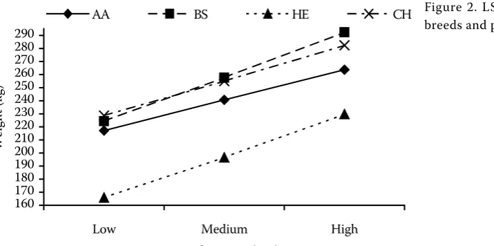
Figure 2 shows the LSM values estimated for breeds at the particular herd levels (G × E interac-tion). The HE breed had the lowest value at all herd levels. The AA, BS and CH breeds had relatively identical values on a low herd level. Differences between the HE and AA breeds decrease with in-creasing herd level. On the other hand, differences in performance between the BS, CH and AA breeds increase and a slight change in the ranking occurs between the BS and CH breeds. This change be-tween the BS and CH breeds may be caused again by the higher lactation performance of the BS breed.
These conclusions demonstrate that weaning weight may be influenced by G × E interaction. The inclusion of interaction in the model did not affect the estimation of residual variability, but it did influence the AIC value, and interaction was found to be a statistically significant effect. The ef-fect of interaction is expressed either as covariance
when a change in environment influences differ-ences between the expected values of genotypes or partly as a change in the ranking of genotypes with similar values.
The results correspond to the definition of G × E interaction according to Lynch and Walsh (1998). The method was used in sheep breeds kept in Norway (Steonheim et al., 2004) and in the Brahman breed and other meat breeds for weaning weight or adult weight (Brown et al., 1993 and Sandelin et al., 2002). Hyde et al. (1998) confirmed the occur-rence of interaction for the Charolais breed under conditions in the USA, Canada, Australia, and New Zealand.
For accurate estimations of the interaction of G × E, models which included covariance between genotype and environment were also tested. These models showed no meaningful results.
Genotype × environment interaction in the definition of environment according to LFA methodology
Further testing of interaction was performed by the estimation of genetic parameters. Table 4 shows the variance-covariance components and genetic parameters with mean errors calculated by the method of the single-trait animal model for the definition of environment according to LFA methodology.
[image:6.595.74.432.84.262.2]Genotype × environment interactions. Models with G × E interaction (Models I, II, III) had slight-ly higher residual variance compared to models without this interaction (Models Ia, IIa, IIIa). The Figure 2. LSM values according to breeds and performance level
160 170 180 190 200 210 220 230 240 250 260 270 280 290
Low Medium High
Performance level
W
ei
gh
t (
kg
)
AA BS HE CH
170 180 190 200 210 220 230 240 250 260 270
Mountain Barely cultivable land Productive Locality
W
ei
gh
t (
kg
)
413 most marked difference was observed in Models
II and IIa, where HYS is considered as a random effect. The value of G × E interaction is reduced to the greatest extent by direct effect and by the effect of breed. The reduction of the above-men-tioned components of variance corresponds to the nature of G × E interaction because the effect of breed is taken as a genetic effect. Besides these effects, G × E interaction in the other models is also reduced by HYS effect. The inclusion of the effect of G × E interaction in the model does not influence either the variance of maternal effect or the variance of the effect of permanent maternal environment. On the other hand, G × E interac-tion decreases the value ram. A decrease in ram is caused by a decrease in the value of variance of the direct effect of G × E interactions. A compari-son of AIC values between the identical models with G × E interaction (Models I, II, III) and mod-els without this interaction (Modmod-els Ia, IIa, IIIa)
shows that the models with G × E interaction had lower values of AIC, which proves the suitability of the inclusion of G × E interaction. The LR values indicated a statistical significance of G × E inter-action only in Model II (P < 0.0001). In the other Models (I, III) G × E interaction was statistically insignificant (P = 0.137, 0.202). G × E interaction explained from 4% (Model II) to 9% (Models I and III) of the total phenotype variability.
[image:7.595.68.532.113.382.2]Fixed or random effect of HYS. A decrease in residual variance was determined in models with random effect HYS (Models II and IIa) compared to the other models (Model I, Ia, III, IIIa). However, in the former models there was an increase in direct and maternal effect and also in the value ram. The increase of direct and maternal effect and genetic correlation (ram) indicates the lower suitability of random effect HYS. The use of fixed HYS was also recommended by Visscher and Goddard (1992) and Hagger (1998).
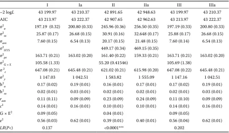
Table 4. Estimations of genetic parameters and their mean errors for Model I–VIIa within the definition of environ-ment according to LFA methodology
I Ia II IIa III IIIa
–2 logL 43 199.97 43 210.37 42 891.65 42 948.63 43 199.97 43 210.37 AIC 43 213.97 43 222.37 42 907.65 42 962.63 43 213.97 43 222.37 σ2
a 197.19 (0.32) 200.80 (0.33) 245.96 (0.36) 256.50 (0.35) 197.19 (0.33) 200.80 (0.33) σ2
m 25.87 (0.17) 26.68 (0.15) 30.91 (0.16) 32.648 (0.17) 25.88 (0.17) 26.68 (0.15) σam 7.60 (0.15) 6.54 (0.13) 20.17 (0.15) 21.48 (0.15) 7.60 (0.14) 6.54 (0.13) σ2
HYS 449.17 (0.34) 469.15 (0.35)
σ2
pe 163.71 (0.21) 163.02 (0.20) 161.40 (0.22) 159.33 (0.21) 163.71 (0.21) 163.02 (0.20) σ2
G × E 105.58 (1.33) 55.20 (0.41546) 105.69 (1.38)
σ 2
e 647.08 (0.21) 645.48 (0.21) 621.02 (0.21) 615.98 (0.20) 647.08 (0.22) 645.48 (0.21) σ2
y 1 147.03 1 042.51 1 583.82 1 555.09 1 147.16 1 042.51 h2
a 0.17 (0.02) 0.19 (0.01) 0.16 (0.01) 0.17 (0.01) 0.17 (0.02) 0.19 (0.01) h2
m 0.02 (0.01) 0.03 (0.01) 0.02 (0.01) 0.02 (0.01) 0.02 (0.01) 0.03 (0.01)
ram 0.11 (0.11) 0.09 (0.09) 0.23 (0.09) 0.24 (0.09) 0.11 (0.10) 0.09 (0.09)
c2 0.14 (0.01) 0.16 (0.01) 0.10 (0.01) 0.10 (0.01) 0.14 (0.01) 0.16 (0.01)
G × E2 0.09 (0.05) 0.04 (0.01) 0.09 (0.05)
e2 0.56 (0.03) 0.62 (0.01) 0.39 (0.01) 0.40 (0.01) 0.56 (0.04) 0.62 (0.01)
LR(P<) 0.137 <0.0001*** 0.202
σ2
a – additive genetic variance of direct effect; σ2m – additive genetic variance of maternal effect; σam – covariance between
direct and maternal effect; ram – genetic correlation between direct and maternal effect;σ2
p e – variance of permanent maternal environment;σ2
H YS – variance of HYS effect; σ2e – variance of random error; σ2y – phenotype variance; h2a – coefficient of direct heritability; h2
m – coefficient of maternal heritability; c2 – ratio of permanent maternal environment; G × E2 – coef-ficient of the effect of genotype × environment interaction; e2 – ratio of residual variance; –2 logL – likelihood function;
Original Paper Czech J. Anim. Sci., 53, 2008 (10): 407–417
Genetic correlations between direct and ma-ternal effects. All models had low positive values of ram estimation. These positive values are caused by the low value of the estimation of maternal ef-fect. The estimations of ram were not statistically significant with respect to their standard errors. The lowest values were computed for Model IIIa (0.09), whereas models with random HYS had the highest values (Models II, IIa) (0.23–0.24).
Direct and maternal heritability coefficients. The values of the coefficient of direct heritability in the set for the estimation of G × E interaction ranged from 0.16 (Model II) to 0.19 (Model Ia). These differences between the models are caused to the greatest extent by the value of phenotypic vari-ance. The value of phenotypic variance is mostly influenced by inclusion or non-inclusion of random effects (HYS and G × E interaction) which were considered as fixed effects in other models. The values of direct and residual variance are identical in the models compared, differing from each other in these effects. Models with G × E interaction had lower values of direct heritability due to the absence of variance of direct effect. On the other hand, iden-tical values were estimated for the coefficient of maternal heritability in most models. The excep-tions were Models I and Ia. Coefficients of maternal heritability had low values in all models, and they did not reach statistical significance similar to ram
when their standard errors were compared.
Genotype × environment interaction in the definition of environment according to herd level
Table 5 shows the estimations of variance-cov-ariance components and genetic parameters with mean errors performed by the method of the sin-gle-trait animal model for the definition of environ-ment according to herd level.
Genotype × environment interactions. Compared to the other models (Models Ia, IIa, IIIa), models with G × E interaction (Models I, II, III) had the same residual variance in most models. The value of residual variance increased only in models with random HYS and G × E interaction (Model II), indicating the lower suitability of G × E interaction in these models. Model IIa with random HYS and without G × E interaction had the lowest value of residual variance. Only slight decreases in the values of residual variance were recorded
in the other models. The addition of G × E inter-action does not improve the explanation of total variability, but rather, there is only an exchange of values between the components. On the contrary, the inclusion of G × E interaction in the model re-duced the variance of direct effect. The greatest difference was determined in Models II (191.47) and IIa (256.50). A marked change in the values of direct effect was also observed in Models I and Ia. The inclusion of G × E interaction in the model also decreased the component for HYS.The addition of random effect HYS increased G × E interaction (Model I vs. II). The reduction of the variance of direct effect through G × E interaction (in Models I and II) corresponds to the definition of G × E in-teraction. G × E interaction also causes an increase in the value ram (Models I and II). This increase is due to a marked decrease in direct effect and a slight decrease in maternal effect. Similarly like the maternal effect, the effect of permanent maternal environment reacts by a slight decrease to the pres-ence of the effect of G × E interaction. Comparison of AIC values between the models with G × E in-teraction (Models I, II and III) and those without this interaction (Models Ia, IIa and IIIa) shows that the models with G × E interaction had lower AIC values. These lower AIC values demonstrate the greater suitability of models with G × E interac-tion. Statistical significance of G × E interaction in Models I and II was confirmed by LR (P = < 0.0001 and < 0.0001). The significance of G × E interac-tion was not proved in the remaining Model (III). G × E interaction explained from 3% (Model III) to 39% (Model II) of the total phenotype variance. The values of residual variance components and selection criteria (AIC, LR) confirm the occurrence of the effect of G × E interaction.
415 assessment of direct and maternal effect and
ge-netic correlation (ram). These conclusions are con-sistent with the results published by Hagger (1998) and Visscher and Goddard (1992). A comparison of
ram and their mean errors shows that all estimations of ram were statistically insignificant again.
Direct and maternal heritability coefficients. The coefficients of direct heritability ranged from 0.09 (Model II) to 0.19 (Model Ia). The inclusion of G × E interaction contributed to a decrease in the coefficient of direct heritability. This decrease was caused by the above-mentioned decrease in the direct effect through G × E interaction. The remaining differences were due to different phe-notype variance. Different values of phephe-notype variance were not caused by different estimations of variance components but by the inclusion of some random effects which were considered as fixed effects in the other models. Identical values were again estimated for direct and residual
vari-ance in the models compared, differing in these above-mentioned effects. On the other hand, the coefficient of maternal heritability had identical values in most models. These identical estimates of maternal heritability coefficients are explained by the low value of maternal effects. The estimates of maternal heritability coefficients were statistically insignificant in most models when their standard deviations were compared.
In both methods of G × E interaction classifica-tion (according to LFA and herd level), the estima-tions of residual variance reached similar values in all the models used. These results indicate that the addition of the effect of G × E interaction does not improve the explanation of variability, only that the values are exchanged among the components.
[image:9.595.65.538.115.395.2]The values of direct heritability coefficient for the most part corresponded to those reported by other authors (Waldron et al., 1993; Robinson, 1996; Meyer, 1997), who estimated the values of Table 5. Estimations of genetic parameters and their mean errors for Model I–VIIa within the definition of environ-ment according to herd level
I Ia II IIa III IIIa
–2 logL 47 289.80 47 427.77 41 271.78 42 948.63 47 276.81 47 283.53 AIC 47 303.8 47 439.77 41 287.78 42 965.63 47 290.81 47 295.53 σ2
a 187.46 (0.32) 198.52 (0.32) 191.47 (0.29) 256.50 (0.35) 187.16 (0.29) 187.64 (0.31) σ2
m 23.76 (0.14) 24.54 (0.15) 24.38 (0.15) 32.65 (0.17) 23.79 (0.15) 24.01 (0.14) σam 9.61 (0.13) 6.50 (0.13) 22.95 (0.12) 21.48 (0.14) 9.60 (0.13) 9.71 (0.12) σ2
HYS 78.70 (0.08) 469.15 (0.35)
σ2
pe 156.66 (0.19) 157.08 (0.21) 168.35 (0.20) 159.33 (0.21) 156.66 (0.19) 156.76 (0.18) σ2
G × E 450.49 (3.36) 730.60 (3.89) 30.72 (0.40)
σ2
e 636.98 (0.20) 636.32 (0.20) 649.46 (0.20) 615.98 (0.20) 637.15 (0.20) 637.24 (0.20) σ2
y 1 464.95 1 022.96 1 865.92 1 555.09 1 045.07 1 015.35 h2
a 0.13 (0.02) 0.19 (0.01) 0.10 (0.01) 0.17 (0.01) 0.18 (0.01) 0.18 (0.01)
h2
m 0.02 (0.005) 0.02 (0.01) 0.01 (0.003) 0.02 (0.01) 0.02 (0.01) 0.02 (0.01)
ram 0.14 (0.10) 0.09 (0.09) 0.34 (0.10) 0.24 (0.09) 0.14 (0.10) 0.14 (0.09) c2 0.11 (0.01) 0.15 (0.01) 0.09 (0.01) 0.10 (0.01) 0.15 (0.01) 0.15 (0.01)
G × E2 0.31 (0.08) 0.39 (0.06) 0.03 (0.02)
e2 0.43 (0.05) 0.62 (0.01) 0.35 (0.04) 0.40 (0.01) 0.61 (0.02) 0.63 (0.01)
LR(P<) <0.0001*** <0.0001*** 0.513
σ2
a – additive genetic variance of direct effect; σ2m – additive genetic variance of maternal effect; σam – covariance between direct and maternal effect; ram – genetic correlation between direct and maternal effect;σ2pe – variance of permanent mater-nal environment;σ2
H YS – variance of HYS effect; σ2e – variance of random error; σ2y – phenotype variance; h2a – coefficient of direct heritability; h2
m – coefficient of maternal heritability; c2 – ratio of permanent maternal environment; G × E2 – coef-ficient of the effect of genotype × environment interaction; e2 – ratio of residual variance; –2 logL – likelihood function;
Original Paper Czech J. Anim. Sci., 53, 2008 (10): 407–417
direct heritability coefficients in the range from 0.15 to 0.40.
Genetic correlations (ram) estimated in our study had low positive values which for the most part are consistent with the those published by Waldron et al. (1993), Robinson (1996), Meyer (1997), and De Mattos et al. (2000) (from –0.594 to 0.223). Van Vleck et al. (1996) stated that correlation coefficients in particular breeds might differ considerably from each other. In agreement with this finding, Meyer (1992) published different estimates of ram for the Hereford (–0.587) and Angus (0.223) breeds.
The values of variance components and selection criteria (AIC, LR) in the definition of environment according to LFA methodology and herd level con-firm the existence of G × E interaction. The with-in-breed interaction was not demonstrated in a previous paper (Vostrý et al., 2007).
The results of this paper showed that the assign-ment of different breeds to specific environassign-ments is questionable under conditions in the Czech Republic. Furthermore, the routine evaluation of animals across all breeds kept in the Czech Republic and all environments also seems to be questionable. The evaluation of animals within breeds could yield more reasonable results.
CONCLUSION
The most suitable definition of environment is that according to herd level. This definition had the most suitable values of residual variance, de-termination coefficient or AIC, and number of connecting sires and their offspring. The defini-tion of environment according to LFA was also recommended because in this methodology both the altitude and the economic value of farm land are considered and also because it is currently used for the allocation of support to farmers.
The weaning weight of beef breeds kept in the Czech Republic is influenced by G × E interaction. G × E interaction was statistically highly significant in the given model. The inclusion of interaction in the model did not change the value of residual variance, but it influenced the AIC value.
The most suitable model for the estimation of G × E interaction and genetic parameters in the definition of environment according to LFA and herd level was Model Ia, which comprised the fixed effect of mother’s age, the combined effect of sex and litter size, the fixed effect of HYS, and
random effects: direct genetic effect of the indi-vidual, direct maternal effect, effect of permanent environment, G × E interaction, and the effect of random error.
The values of variance components and selection criteria (AIC, LR) indicated that G × E should be taken into consideration in evaluation of the wean-ing weight of beef cattle.
REFERENCES
Brown M.A., Brown A.H., Jackson W.G., Miesner J.R. (1993): Genotype × environment interactions in post-weaning performance to yearling in Angus, Brahman and reciprocal-cross calves. Journal of Animal Science, 71, 3273–3279.
Bozdogan H. (2000): Akaike’s information criterion and recent developments in information complexity. Jour-nal of Mathematical Psychology, 44, 62–91.
De Mattos D., Bertrand J.K., Misztal I. (2000): Investiga-tion of genotype × environment interacInvestiga-tions for wean-ing weight for Herefords in three countries. Journal of Animal Science, 78, 2121–2126.
Falconer D.S. (1970): Introduction to quantitative genet-ics. Oliver and Boyd, London, UK, 365 pp.
Fernando R.F., Knights S.A., Gianola D. (1984): On a method of estimating the genetic correlation between characters measured in different experimental units. Theoretical and Applied Genetics, 67, 175–178. Hagger C. (1998): Litter, permanent environmental,
ram-flock, and genetic effects on early weaning gain of lambs. Journal of Animal Science, 76, 452–457. Hyde L.R., Bourdon R.N., Golden B.L., Comstok C.R.
(1998): Genotype by environment interaction for growth and milk traits in an international population of Cha-rolais cattle. Journal of Animal Science, 76, 60. Kaps M., Lamberson W. (2004): Biostatistics for Animal
Science. CABI Publishing, UK, 445 pp.
Kolmodin R., Strandberg E., Madsen P., Jensen J., Jorjani H. (2002): Genotype by environment interaction in Nordic dairy cattle studied using reaction norms. Acta Agriculturae Scandinavica, Section A – Animal Sci-ences, 52, 11–24.
Kovač M., Groeneveld E., García-Cortes L.A. (2002): VCE-5 A package for the estimation of dispersion pa-rameters. In: Proc. 7th WCGALP, CD ROM,
Commuta-tion, No. 8-06.
417 Křížek J., Rais I., Říha M. (1992): Genotype × environment
interactions under different conditions of set – stock-ing in sheep. Archiv fur Tierzucht, 6, 619–628. Lin C.Y., Togashi K. (2002): Genetic improvement in the
presence of genotype by environment interaction. Jour-nal of Animal Science, 73, 3–11.
Lynch M., Walsh B. (1998): Genetics and analysis of quan-titative trait. Sinauer Associates, 971 pp.
Mathur P.K., Schlote W. (1995): Univariate or multivar-iate approach for estimating genotype – environment interactions? Archiv fur Tierzucht, 38, 577–586. Meyer K. (1992): Variance components due to direct and
maternal effects for growth traits of Australian beef cattle. Livestock Production Science, 31, 179–204. Meyer K. (1997): Estimates of genetic parameters for
weaning weight of beef cattle accounting for direct-maternal environmental covariances. Livestock Pro-duction Science, 52, 187–199.
Notter D.R., Tier B., Meyer K. (1992): Sire × herd interac-tions for weaning weight in beef cattle. Journal of Animal Science, 70, 3259–2365.
Přibyl J., Misztal I., Přibylová J., Šeba K. (2003): Multiple-breed, multiple-traits evaluation of beef cattle in the Czech Republic. Czech Journal of Animal Science, 48, 519–532.
Rasch D., Mašata O. (2006): Methods of variance com-ponent estimation. Czech Journal of Animal Science, 51, 227–235.
Robinson D.L. (1996): Estimation and interpretation of direct and maternal genetic parameters for weights of Australian Angus cattle. Livestock Production Science, 45, 1–11.
Sandelin B.A., Brown A.H., Brown M.A., Johanson Z.B., Kellogg D.W., Stelzleni A.M. (2002): Genotype × envi-ronmental interaction for mature size and rate of
ma-turing for Angus, Brahman, and reciprocal-cross cows grazing bermudagrass or endophyte infected rescue. Journal of Animal Science, 80, 3073–3076.
SAS (2004): SAS/STAT® 9.1 User’s Guide. Cary, NC. SAS
Institute Inc., 5121 pp.
Steonheim G., Adnoy T., Meuwissen T., Klemetsdal G. (2004): Indications of breed by environment interaction for lamb weights in Norwegian sheep breeds. Acta Ag-riculturae Scandinavica, Section A – Animal Sciences, 54, 193–196.
Van Vleck L.D., Gregory K.E., Bennett G.L. (1996): Direct and maternal genetic covariances by age of dam for weaning weight. Journal of Animal Science, 74, 1801–1805.
Visscher P.M., Goddard M.E. (1992): Fixed and random contemporary groups. Journal of Dairy Science, 76, 1444–1454.
Veselá Z., Přibyl J., Vostrý L., Štolc L. (2007): Stochastic simulation of the influence of insemination on the es-timation of breeding value and its reliability. Czech Journal of Animal Science, 52, 236–248.
Vostrý L., Přibyl P., Veselá Z., Jakubec V. (2007): Selection of a suitable data set and model for the estimation of genetic parameters of the weaning weight in beef cat-tle. Archiv für Tierzucht, 50, 562–574.
Willham R.L. (1979): The role of maternal effects in ani-mal breeding: III. Biometrical aspects of maternal ef-fects in animals. Journal of Animal Science, 35, 1972–1293.
Waldron D.F., Morris C.A., Baker R.L., Johanson D.L. (1993): Maternal effects for growth traits in beef cattle. Livestock Production Science, 34, 57–70.
Received: 2007–10–04 Accepted after corrections: 2008–03–21
Corresponding Author
Ing. Luboš Vostrý, Ph.D, Czech University of Life Sciences Prague, Kamýcká 129, 165 21 Prague 6-Suchdol, Czech Republic