The Lyman alpha luminosity function at z=5 7 6 6 and the steep drop of the faint end:implications for reionization

The Ly

α

luminosity function at z

=

5

.

7

₋

6

.

6 and the steep

drop of the faint end: implications for reionization

S´ergio Santos

_{, David Sobral}

_{& Jorryt Matthee}

1 _{Instituto de Astrof´ısica e Ciˆencias do Espa¸co, Universidade de Lisboa, OAL, Tapada da Ajuda, PT1349-018 Lisboa, Portugal} 2 _{Departamento de F´ısica, Faculdade de Ciˆencias, Universidade de Lisboa, Edif´ıcio C8, Campo Grande, PT1749-016 Lisbon, Portugal} 3 _{Department of Physics, Lancaster University, Lancaster, LA1 4YB, UK}

4 _{Leiden Observatory, Leiden University, P.O. Box 9513, NL-2300 RA Leiden, The Netherlands}

23 August 2016

ABSTRACT

We present new results from the widest narrow band survey search for Lyαemitters at

z= 5.7, just after reionization. We survey a total of 7 deg2_{spread over the COSMOS,}

UDS and SA22 fields. We find over 11,000 line emitters, out of which 514 are robust Lyαcandidates atz= 5.7 within a volume of 6.3_×106_Mpc3_{. Our Lyαemitters span}

a wide range in Lyαluminosities, from faint to bright (LLyα∼1042.5−44erg s−1) and

rest-frame equivalent widths (EW0 ∼ 25−1000 ˚A) in a single, homogeneous

data-set. By combining all our fields we find that the faint end slope of the z = 5.7 Lyα

luminosity function is very steep, with α = ₋2.3+0₋₀._.4₃. We also present an updated

z= 6.6 Lyαluminosity function, based on comparable volumes and obtained with the same methods, which we directly compare with that atz= 5.7. We find a significant decline of the number density of faint Lyα emitters from z = 5.7 to z = 6.6 (by 0.5_±0.1 dex), but no evolution at the bright end/no evolution inL∗. Faint Lyαemitters at z = 6.6 show much more extended haloes than those at z = 5.7, suggesting that neutral Hydrogen plays an important role, increasing the scattering and leading to observations missing faint Lyαemission within the epoch of reionization. All together, our results suggest that we are observing patchy reionization which happens first around the brightest Lyαemitters, allowing the number densities of those sources to remain unaffected by the increase of neutral Hydrogen fraction fromz_∼5 toz_∼7.

Key words: galaxies: high-redshift – galaxies: luminosity function – cosmol-ogy:observations – cosmology: dark ages, reionization, first stars.

1 INTRODUCTION

During the past two decades, considerable progress has been made in understanding the distant/early Universe (see re-views by e.g. Robertson et al. 2010; Dunlop et al. 2012; Madau & Dickinson 2014). Currently, the samples ofz >6 candidates are mostly composed by rest-frame ultra-violet (UV) selected galaxies obtained from extremely deep surveys with the Hubble Space Telescope (e.g.Bouwens et al. 2015; Finkelstein et al. 2015). However, spectroscopy and multi-wavelength follow-up (e.g. with ALMA; Ouchi et al. 2013; Watson et al. 2015;Capak et al. 2015;Maiolino et al. 2015) of these sources still remains very limited as most candidates are too faint for a detailed analysis with current instrumen-tation (see alsoDunlop et al. 2016). Alternatively, emission lines can be used to search for high-redshift galaxies to di-rectly select galaxies by their brightest features, including

? _{E-mail: [email protected]}

several rest-frame optical and UV lines (e.g. Ouchi et al. 2008; Sobral et al. 2013; Khostovan et al. 2015,2016), al-lowing for efficient follow-up strategies.

The Lyman-α (Lyα) emission line (rest-frame

1215.67 ˚A) is emitted by both young star-forming galaxies and active galactic nuclei/quasars, being intrinsically the strongest emission line in the rest-frame optical to UV (e.g. Partridge & Peebles 1967; Pritchet 1994). As Lyα

is redshifted into optical wavelengths (it can be observed from the ground atz≈2−7), many other strong lines are redshifted out of even the near-infrared (see e.g. Ly et al. 2007, 2011; Hayes et al. 2010; Sobral et al. 2013), making Lyα one of the only available means of spectroscopic confirmation, along with other weaker high ionisation UV lines (e.g.Sobral et al. 2015;Stark et al. 2016).

Several approaches have been used to find and study Lyαemitters, including blind spectroscopy (e.g. Martin & Sawicki 2004; Stark et al. 2007; Rauch et al. 2008; Saw-icki et al. 2008; Bayliss et al. 2010; Cassata et al. 2011),

narrow band surveys (e.g.Cowie & Hu 1998;Rhoads et al. 2000,2003;Malhotra & Rhoads 2004;Taniguchi et al. 2005; Shimasaku et al. 2006; Westra et al. 2006; Iye et al. 2006; Nilsson et al. 2007;Murayama et al. 2007;Ouchi et al. 2008, 2010; Sobral et al. 2009; Hu et al. 2010; Kashikawa et al. 2011;Shibuya et al. 2012;Konno et al. 2014;Matthee et al. 2014,2015) and Integral Field Unit (IFU) observations (e.g. Blanc et al. 2011;Adams et al. 2011;van Breukelen et al. 2005;Bacon et al. 2015;Karman et al. 2015). Blind spec-troscopy and IFU surveys can be very efficient at probing ultra-low luminosity sources at a variety of redshifts, but the current small volumes probed make them unable to reach evenL∗sources, as the rarer (brighter) sources have number densities several times smaller that these studies can reach. Wide narrow band surveys can be very competitive at ef-ficiently probing large volumes at specific look-back times, and can be used to study a much larger luminosity range. For example, one MUSE pointing (e.g. Bacon et al. 2015) probes a volume of ∼ 103_Mpc3 _{for z ∼ 3−6, while one}

Subaru Suprime-Cam pointing with a typical narrow band filter probes a volume of∼105 _Mpc3 _{(Hyper Suprime-Cam}

covers a volume∼ 7 times larger per pointing). Typically, narrow band surveys have targeted a maximum of∼1 deg2 areas, corresponding to maximum volumes of ∼106 Mpc3 (e.g. Ouchi et al. 2008, 2010), but the next generation of surveys are now starting to probe much larger volumes (e.g. Matthee et al. 2015;Hu et al. 2016).

Due to its resonant nature, Lyαphotons are easily scat-tered by neutral hydrogen (and also easily absorbed by dust; e.g.Hayes et al. 2011). As a consequence, the observability of Lyα can in principle be used as a probe of the neutral state of the inter-galactic medium (IGM) during the epoch of reionization (e.g.Fontana et al. 2010;Caruana et al. 2012; Schenker et al. 2012;Ono et al. 2012;Caruana et al. 2014; Dijkstra 2014; Pentericci et al. 2014;Schmidt et al. 2016). However, in order to interpret Lyαobservations (such as the distribution of equivalent widths, the fraction of UV selected galaxies with strong Lyα, or the evolution of the number density of Lyαemitters) as consequences of reionization, one needs to accurately understand the contribution from poten-tially varying intrinsic inter-stellar medium (ISM) properties such as the Lyαescape fraction (c.f.Matthee et al. 2016a), overdensities of galaxies (e.g.Castellano et al. 2016) or selec-tion biases in UV selected galaxy samples (c.f.Oesch et al. 2015;Zitrin et al. 2015; Stark et al. 2016). Therefore, it is important to have a clear understanding of Lyαwith only little influence from the IGM at z ≈6, when reionization is close to complete and the fraction of neutral hydrogen becomes extremely low (Fan et al. 2006;Becker et al. 2015). Previous studies found that the Lyαluminosity function (LF) seems to have little evolution atz∼3−6 (e.g.Ouchi et al. 2008). In contrast, the UV LF of Lyman-break galaxies (LBGs) strongly decreases for higher redshifts (e.g.Bouwens et al. 2015;Finkelstein et al. 2015). This difference in evo-lution is likely explained by an evolving escape fraction of Lyαphotons, likely due to a lower dust content, younger stel-lar populations, lower metallicities and/or a combination of related phenomena. This is consistent with the observation that the fraction of LBGs with strong Lyαemission increases up toz= 6 (e.g.Stark et al. 2010;Cassata et al. 2015). At

z >6 the number density of faint Lyαemitters (LAEs) is found to decline with redshift (Ouchi et al. 2010; Konno

et al. 2014), likely due to reionization not being fully com-pleted. However, by using the largest Lyαsurvey at z ∼7 (∼5 deg2_{),Matthee et al. (2015) show that the strong}

de-crease/evolution in the number density of LAEs happens pre-dominantly at relative faint Lyαluminosities, while the bright end (with luminosities LLyα>1043erg s−1) may not

evolve at all.Matthee et al.(2015) finds that bright LAEs atz= 6.6 are much more common than previously thought, with spectroscopic confirmation presented in Sobral et al. (2015), and with independent studies finding consistent re-sults (see e.g.Hu et al. 2016). However, one strong limita-tion in interpreting the potential evolulimita-tion fromz= 6.6 to

z= 5.7 is the lack of comparably large∼5−10 deg2, multi-ple field surveys that can both trace a large enough number of bright sources and overcome cosmic variance.

In this work, we present the largest Lyαnarrow band survey atz= 5.7, covering a total of∼7 deg2(∼107Mpc3). Previous studies have never probed beyond 2 deg2_(e.g.

Mu-rayama et al. 2007;Ouchi et al. 2008;Hu et al. 2010), and have mostly focused on specific, single fields. Here we take advantage of previous data and add further∼4 deg2 _of

un-explored data. We also re-analyse the z = 6.6 luminosity function presented inMatthee et al.(2015).

We structure this paper as follows: Section2presents the observations and data reduction. Section3explains the selection of line emitters and Lyαemitters at z = 5.7. In Section4we present the method and procedures adopted to construct thez= 5.7 andz= 6.6 LyαLFs. We present our results in Section5, including a comparison with previous surveys. Section6discusses the results in the context of pre-dicted effects from reionization. Finally Section 7presents the conclusions of this paper.

Throughout this work we use a ΛCDM cosmology with H0 = 70 km s−1Mpc−1, ΩM = 0.3 and ΩΛ = 0.7. All

mag-nitudes in this paper are presented in the AB system. At

z= 5.7, 100corresponds to 5.9 kpc.

2 OBSERVATIONS AND DATA REDUCTION

2.1 Observations

We have reduced and analyzed raw archival NB816 data in the COSMOS, UDS and SA22 fields. We use these three fields as they are completely independent (preventing any possible bias from probing the same region of the sky) and far enough from the galactic plane (avoiding bright fore-ground stars and dust). Additionally, the available deep multi-wavelength coverage (including optical and near infra-red) allows a robust selection of candidates and identification of any lower redshift interlopers.

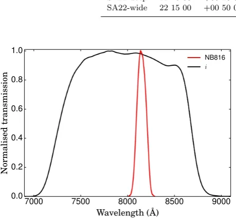
The NB816 filter has a central wavelength of 8150 ˚A and a full width at half maximum (FWHM) of 120 ˚A. NB816 is contained within the red wing of the broad band fil-ter i (see Figure 1). All NB816 data were collected with the Suprime-Cam instrument from the Subaru Telescope

(Miyazaki et al. 2002). Suprime-Cam has ten 2048x4096

Table 1.Our NB816 data in the COSMOS, UDS and SA22 fields. The SA22 field was separated into two sub-fields, deep and wide, according to its significantly different NB816 depth. R.A. and Dec. are the central coordinates of the fields. FWHM is the average value for the seeing and is similar across our entire coverage. The NB816 depth is the 2σdepth measured in 200_{apertures. Note that the quoted}

area already takes into account the removed/masked regions which are not used in this paper.

Field R.A. Dec. Area FWHM NB816 depth

(J2000) (J2000) (deg2_{) (}00_{) (2σ, 2}00₎

COSMOS 10 00 00 +02 10 00 2.00 0.7 26.2

UDS 02 18 00 −05 00 00 0.85 0.7 26.1

SA22-deep 22 18 00 +00 20 00 0.55 0.7 26.1 SA22-wide 22 15 00 +00 50 00 3.60 0.5 25.0

7000 7500 8000 8500 9000

Wavelength ( ˚A)

0.0 0.2 0.4 0.6 0.8 1.0

Normalised

transmission

NB816 i

Figure 1.Normalised filter profiles of the NB816 and theiband filters used in this study. We note that the showniband is for Subaru’s Suprime-Cam after the upgrade to red sensitive CCDs, such that its peak is slightly shifted towards the red compared to the CFHT MegaCami band used for SA22. Our NB correc-tion in Seccorrec-tion2.4.1takes this into account. NB816 is contained slightly red from the center ofi. The NB816 filter is located in a wavelength region free of strong atmospheric OH lines.

the UDS and SA22 fields from the SMOKA Archive1_{. Fully}

reduced COSMOS NB816 images (original PSF) were re-trieved from the COSMOS Archive2(Taniguchi et al. 2007; Capak et al. 2007).

We split SA22 data into two different sub-fields (SA22-deep and SA22-wide), which differ in depth by≈1 mag and in area by a factor of≈6.6. SA22-wide contains the largest area (larger than COSMOS and UDS combined). Narrow band observations are summarized in Table1.

Previous studies have separately used NB816 data in COSMOS (Murayama et al. 2007), UDS/SXDF (Ouchi et al. 2008) and SA22-deep (∼0.4 deg2_{;Hu et al. 2010). We note}

that while we explore new data and provide the largest sur-vey of its kind, we are able to reproduce individual results from the literature using our own analysis. A comparison between our findings and previous studies is presented in Section4.

1 _{http://smoka.nao.ac.jp/}

2 _{http://irsa.ipac.caltech.edu/data/COSMOS/}

2.2 Data reduction

We used the Subaru data reduction pipelines (sfred and

sfred2;Ouchi et al. 2004) to reduce the NB816 data. The

data reduction follows the same procedure as detailed in e.g. Matthee et al.(2015) and we refer the reader to that study for more details. Briefly, the reduction steps include: over-scan and bias subtraction, flat fielding, point spread function homogenisation, sky background subtraction and bad pixel masking. After these steps, we apply an astrometric calibra-tion using_scamp(Bertin 2006) to correct astrometric dis-tortions. The software matches our images with the 2MASS catalog in theJ band (Skrutskie et al. 2006) and fits poly-nomial functions that correct for any distortions along the CCD.

We calibrated the photometry in our data by matching relatively bright, un-saturated stars and galaxies to public catalogues for COSMOS (Laigle et al. 2016), UDS (Cirasuolo et al. 2007) and SA22 (Sobral et al. 2013, 2015; Matthee et al. 2014) using_stilts(Taylor 2006). NB816 images were calibrated usingiband photometry, but a further correction to this calibration was applied in Section2.4.1. Co-added stacks of NB816 exposures were obtained using theswarp

software (Bertin et al. 2002).

We masked low quality regions, bright haloes around bright stars, diffraction patterns and low S/N regions due to dithering strategy (particularly important in SA22-wide). We also removed regions with low quality or absentiband coverage, regardless of the quality of the narrow band.

We note that our masking is very conservative and, con-sequently, a relatively large area is removed from our study (hundreds of arcmin2), but that is still only a small frac-tion of our total area. After masking low quality regions, our NB816 coverage contains a total area of 7 deg2 (Figure 2), corresponding to a comoving volume of 6.3×106_Mpc3

at z = 5.7. All areas and volumes used and mentioned in this paper take into account these masks, unless stated oth-erwise.

Finally, we measure the depth of our images using ran-domly placed 200apertures. In each image, we place 200,000 empty apertures in random positions. The average results per field are given in Table1.

2.3 Multi-wavelength imaging

Sub-149.4 149.6 149.8 150.0 150.2 150.4 150.6 150.8

R.A. (J2000)

1.4 1.6 1.8 2.0 2.2 2.4 2.6 2.8 3.0

D

ec

.(

J2

00

0)

COSMOS

33.8 34.0 34.2 34.4 34.6 34.8 35.0 35.2

RA (J2000)

-5.6 -5.4 -5.2 -5.0 -4.8 -4.6

DEC

(J2000)

UDS

332.0

332.5

333.0

333.5

334.0

334.5

335.0

335.5

R.A. (J2000)

0.0

0.2

0.4

0.6

0.8

1.0

1.2

1.4

1.6

D

ec

.(

J2

00

0)

SA22

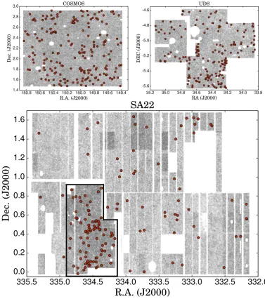
Figure 2.The spatial distribution of sources in the COSMOS, UDS and SA22 fields. Grey dots indicate all detections and red circles identify ourz= 5.7 Lyαemitter candidates. A black line contour identifies SA22-deep, the deepest region in the SA22 field. The figure also highlights the regions masked due to bright stars, bad regions and/or low S/N due to dither strategy. It can be seen that UDS, COSMOS and SA22-deep are the deepest regions with a high concentration of sources and candidate LAEs.

Table 2.Multi-wavelength depths (2σ; measured in 200empty apertures) for the available broad-band filters across all three fields. Field Broad band filters Broad band depth (2σ, 200₎

COSMOS BV grizY J HK 27.6, 27.0, 27.1, 27.0, 26.6, 25.7, 25.3, 24.6, 25.0, 24.7 UDS BV rizJ K 27.5, 27.2, 27.0, 26.8, 27.0, 25.3, 24.8 SA22 ugrizJ K 26.2, 26.5, 25.9, 25.6, 24.5, 24.3, 23.8

aru/SuprimeCam (Taniguchi et al. 2007;Capak et al. 2007),

retrieved from the COSMOS Archive and NIRYHJK data

from UltraVISTA DR2 (McCracken et al. 2012), taken with VISTA/VIRCAM. For the UDS field, we use opticalBVriz data from SXDF (Furusawa et al. 2008) and NIRJHK data from UKIDSS (Lawrence et al. 2007). For the SA22 field we

use opticalugriz data from CFHTLS3, taken with the Mega-Cam (Boulade et al. 2003) and NIRJK data from UKIDSS

DXS (Warren et al. 2007), taken with UKIRT/WFCAM

(Casali et al. 2007). All data which were not taken with the Subaru/SuprimeCam were degraded to a pixel scale of

20 21 22 23 24 25 N B816(AB magnitude)

-1 0 1 2 3

i

NB

816 _EW

0= 25 ˚A

SA22-deep

Line-emitters

z⇠5.7LAEs

20 21 22 23 24

N B816(AB magnitude) -1

0 1 2 3

i

NB

816 _EW 0= 25 ˚A

SA22-wide

Line-emitters

z⇠5.7LAEs

20 21 22 23 24 25

N B816(AB magnitude)

-1 0 1 2 3

i

NB

816

EW0= 25 ˚A

COSMOS

Line-emitters

z⇠5.7LAEs

20 21 22 23 24 25 26

N B816(AB magnitude)

-1 0 1 2 3

i

NB

816

EW0= 25 ˚A

UDS

Line-emitters

z⇠5.7LAEs

COSMOS (2 deg

₎

_{UDS (0.85 deg}

₎

SA22-wide (3.6 deg

₎

SA22-deep (0.55 deg

₎

Σ>3 (average) Σ>3 (average)

Σ>3 (average) Σ>3 (average)

Figure 3.Narrow band excess diagram for COSMOS, UDS and SA22. We plot narrow band excess (i broad band magnitude minus NB816 magnitude) versus narrow band NB816 magnitude. Grey points represent all detections after masking, removal of sources with non-physical narrow band and cosmic rays. Green points represent line-emitters, obtained by applying the EW and Σ cuts described in Section3. For visual reference, we collapsed the points with no i detection in the top region of the plots. The Σ line shown in this figure is the median value from small sub-fields which we created inside each field.

0.2000pix−1_using

swarp. A summary of the available filters

for each field and their photometric depth is shown in Table 2.

2.4 NB816 catalogue

The extraction of sources was conducted using SExtrac-tor(Bertin & Arnouts 1996) in dual extraction mode, using

NB816 as the detection image.

2.4.1 Narrow band magnitude correction

The NB816 filter is located slightly to the red of the Sub-aru Suprime-cam ifilter (with red sensitive CCDs) with a separation of≈180 ˚A between the center of the two filters. Calibrating the narrow band magnitude directly to the i

band may result in an offset in the magnitudes, particularly for sources with strong colours. We correct the narrow band magnitudes by summing a small correction factor which is estimated from the color of the two adjacent broad bands,

iandz. To compute this correction, we use sources withi,

zand NB816 magnitudes between 19 and 24 (not saturated and with high enough S/N). The correction has the following expression:

N Bcorrected=N B+ 0.4×(i−z), (1)

whereN B,iandz are the 200magnitudes in the respective bands andN Bcorrected is the corrected NB816 magnitude. We apply this correction to sources withiandzdetections. For the remaining sources, we apply a median correction of +0.20. As a result of this correction, there is less scatter in the excess diagram (Figure3). The correction also corrects for the fact that the CFHT MegaCamiband is slightly bluer than Suprime-cam’siband, because this slightly differenti

band will result in slightly differenti−z colours.

Our narrow band correction is an alternative to the correction applied in Murayama et al. (2007) who used a corrected broad band obtained from an iz interpolation. Our narrow band correction corresponds to aBBcorrected= 0.6i+ 0.4zwhich is fully consistent with their interpolation.

2.4.2 Removal of sources with non-physical narrow band detection

The wavelengths covered by NB816 are contained inside the

iband coverage. This means that sources with NB816 de-tection should be detected in i as long as the i image is deep enough. For each source we compute the expected i

sources (such as supernovae and moving sources) and spu-rious sources that are detected only in the narrow band im-ages and sources with boosted narrow band emission from e.g. diffraction patterns.

2.4.3 Cosmic ray removal

Cosmic rays may become artefacts in images. This problem can be avoided through stacking of several frames. How-ever, in our shallower SA22-wide data, the small number of frames causes a less efficient removal of such artefacts dur-ing stackdur-ing. We created an automated procedure to identify and remove cosmic rays from our sample.

For each source detected in the NB816 imaging we mea-sure the standard deviation in boxes of 5×5 pixels around each source. Cosmic rays can be easily identified by their high standard deviation, several times higher than any real source. We apply a cautious cut to make sure we do not lose any real sources. Since we were cautious with this step, we also visually inspect all the final LAE candidates to identify any cosmic ray that was not excluded.

3 SELECTING NB816 LINE EMITTERS

For the selection of line-emitters, we apply similar criteria to e.g.Sobral et al.(2013) andMatthee et al.(2015), relying on two parameters: equivalent width (EW) and Sigma (Σ). The equivalent width is the ratio between the flux of an emission line and the continuum flux. It can be expressed as:

EWobs= ∆λN B fN B−fBB

fBB−fN B(∆λN B/∆λBB), (2) where ∆λN Band ∆λBBare the FWHM of the narrow band and broad band filters (∆λN B816 =120 ˚A; ∆λi =1349 ˚A)

andfN BandfBBare the flux densities measured in the two filters.

The second parameter, Sigma (Σ, e.g. Bunker et al. 1995), is used to assure that the excess of the NB816 rel-ative to the broad-band is significantly above the noise. It can be written as (Sobral et al. 2013):

Σ = 1−10

−0.4(BB−N B)

10−0.4(ZP−N B)p rms2

BB+rms 2 N B

(3)

where BB and NB are the broad band and the corrected narrow band magnitudes (in this case, NB816 andi), ZP is the zero-point of the image (set to 30) and rms is the root-mean-square of the background of the respective image.

To select our sample of line-emitters, we apply the fol-lowing selection criteria:

• i−N B816>0.8

• Σ>3

The narrow band excess criteriai−N B816>0.8 cor-responds to a rest-frame EW of 25 ˚A for a z = 5.7 LAE. This cut is similar to the one used byHu et al.(2010) and Matthee et al.(2015) forz= 6.6 but slightly lower than e.g. Ouchi et al.(2008) (i−N B816>1.2) andTaniguchi et al. (2005) (i−N B816>1).

We present the narrow band excess diagram in Figure3,

0 1 2 3 4 5 6

Photometric redshift

5% 10% 15% 20% 25%

Pe

rcentage

of

line-emitters

H

α

[O

]

[O

]

Ly

α

Figure 4.Distribution of photometric redshifts of line-emitters selected in COSMOS, UDS and SA22 by using a simple selection criteria ofi−N B186>0.25 and Σ>3. The peaks are consistent with line emission at specific wavelengths. Annotations indicate the redshifts where we expect major emission lines (Hαatz∼0.2, [Oiii] at∼0.6, [Oii] atz∼1.2 and Lyαatz= 5.7).

highlighting our sample of line-emitters. With our selection criteria we identify over 11,000 candidate line emitters.

3.1 Photometric and spectroscopic redshifts

In order to explore the nature of the line-emitters, we have used accurate photometric redshifts and a large compilation of spectroscopic redshifts:Laigle et al.(2016) for COSMOS, Cirasuolo et al.(2007) for UDS and a combination ofKim et al.(2015),Matthee et al.(2014) andSobral et al.(2015) for SA22. We retrieve∼5000 emitters with either available photometric or spectroscopic redshift. Figure4presents the distribution of photometric redshifts of our sample of line emitters. Even though our high EW cut is tuned to select Lyαemitters atz = 5.7, our initial sample of line emitters reveals a range of strong line emitters. The peaks in the photometric redshifts are consistent with Hα at z ∼ 0.2,

[Oiii]at∼0.6,[Oii] atz ∼1.2 and Lyαat z = 5.7. From

our spectroscopic redshift, we find a total of 46 Lyαemitters atz= 5.7.

As expected, our sample is dominated by lower redshift line-emitters, mostly composed by sources up toz∼1.2. In order to isolate LAEs at z= 5.7 from our sample we require additional selection criteria, which we will explore in Section 3.2.

3.2 Selection of LAEs at z=5.7

there are few Lyαforest lines). To summarise, we apply the following criteria, similar toOuchi et al.(2008):

B > B2σ∧V > V2σ∧[r > r2σ∨(r < r2σ∧r−i >1.0)] (4)

whereB,V,randiare the 200magnitudes in the respective bands and the 2σ subscript indicates the 2σ depth for the

images of the respective bands (see Table2). As there are no availableBV data over the full SA22, we apply a small variation of Equation4where useuginstead:

u > u2σ∧g > g2σ∧[r > r2σ∨(r < r2σ∧r−i >1.0)] (5)

where u,g are the 200 magnitudes in the respective bands. This criteria ensures we select sources with no detection in the BV ugbands but can have some detection inr as long as there is a strongi−rcolor break.

In extreme cases, z ∼ 1 line emitters with a strong Balmer-break could mimic the Lyman-break that we detect. Fortunately, those sources can be identified by their red col-ors. Similar toMatthee et al.(2015) we reject sources which have significant red colors in the observed NIR bands. Thus, we consider sources withJ−K >0.5 to be interlopers. This additional NIR criterion is most important in SA22, where the optical data are relatively shallow.

In order to ensure that our candidates are real detec-tions and not spurious sources, we visually inspect each one of the remaining candidates. We first inspect sources in the narrow band images and reject any fake detections (usually originated by e.g. diffraction patterns from bright sources which were not completely masked). We also visually check that each source does not have an optical detection blue-ward of the Lyman-break. To do so, we create an optical stack using the available optical bands for each field (BVg for COSMOS,BV for UDS andugfor SA22), which signif-icantly increases the depth of our images.

To summarise, we select line-emitters as Lyαatz= 5.7 if:

• They have no optical detection blue-ward of the Lyman-break (Equation4or5).

• They satisfyJ−K <0.5, if detected in the NIR.

• They pass visual inspection, which includes both reality of NB excess (and checking for variability and/or moving sources) and no detection in optical bands.

3.3 Comparison with other samples of Lyα emitters at z=5.7

We compare our sample of LAEs with the spectroscopically confirmed sources atz= 5.7 provided byOuchi et al.(2008) (UDS), Hu et al. (2010) (SA22-deep) and Mallery et al. (2012) (COSMOS). We find that we recover 46 spectro-scopically confirmed sources from previous studies which are above our conservative Σ detection threshold (other studies typically only apply an EW cut) and that are not in our conservative masked regions.

3.4 Final sample of Lyαemitters at z=5.7

Across the COSMOS, UDS and SA22 fields we identify a total of 514z= 5.7 LAE candidates (currently 46 are spec-troscopically confirmed), spanning a range of Lyα luminosi-ties of 1042.5₋₁₀44_{erg s}−1_{. We will explore the properties}

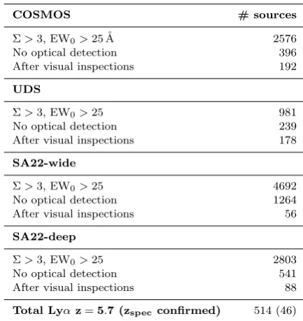
Table 3. Number of candidates after each selection step. The visual inspections step includes individually checking each source first in both the narrow band NB816 and the broad bandiimages and then for no detection in the deep optical stacks (BV for UDS,BV gfor COSMOS andugfor SA22). Note that due to the shallower broad band data in SA22, a large amount of sources passed the initial filtering, but are rejected with the much deeper ugstacks and our visual checks.

COSMOS # sources

Σ>3, EW0>25 ˚A 2576

No optical detection 396

After visual inspections 192

UDS

Σ>3, EW0>25 981

No optical detection 239

After visual inspections 178

SA22-wide

Σ>3, EW0>25 4692

No optical detection 1264

After visual inspections 56

SA22-deep

Σ>3, EW0>25 2803

No optical detection 541

After visual inspections 88

Total Lyαz=5.7 (zspec confirmed) 514 (46)

of these sources in the following sections. Table3 shows a summary of the number of sources after each selection cri-terion. The spatial distribution of the LAEs in all fields can be seen in Figure2.

4 COMPUTING THE LYαLF

4.1 Completeness correction

4.2 Filter profile correction

The narrow band filter transmission NB816 has a gaussian distribution with a lower transmission in the wings (Figure 1). Sources which have a redshift in the borders of the filter will only be observed at a fraction of their Lyαluminosity (see e.g.Hu et al. 2010). It is necessary to apply a correction factor that compensates the fact that the filter is not top-hat, otherwise, the number densities of bright LAEs will be systematically underestimated. We apply a correction simi-lar to Matthee et al.(2015). We use the Schechter fit from our data to generate the Lyαluminosity of 1 million sources at a random redshift betweenz= 5.65 andz= 5.75 (corre-sponding to the edges of NB816). For each luminosity bin, the correction factor is determined from the detection ratio of these fake sources retrieved with the two different filter profiles. The effect of the filter profile correction of our LF is shown in FigureA1. The correction is higher for the bright-est bins as these LAEs will likely be observed at a fraction of their luminosity due to the filter not being top-hat.

4.3 Aperture corrections

Due to instrumental/observational effects (e.g. seeing/PSF) and mostly due to Lyα photons easily scattering within haloes, Lyα flux can be significantly extended (e.g. Mo-mose et al. 2014;Wisotzki et al. 2016;Matthee et al. 2016a; Borisova et al. 2016). The 200 apertures we use are 3−4×

the PSF, and thus for point-like sources we do not expect aperture corrections to be important, but if sources are phys-ically extended, 200apertures may lead to missing flux. We investigate this by comparing the NB816 fluxes measured in 200 with those measured with_mag-auto and study any necessary correction as a function of observed 200 flux. We find little to no dependence up to at least the highest fluxes, and derive a median correction of +0.02 in Lyαluminosity, which we apply (see further discussion in Section5.3).

4.4 Interloper correction

While in COSMOS and UDS the available broad-band data allows to clearly identify and remove interlopers/lower red-shift line emitters, in SA22 this is not necessarily the case, particularly for the sources with the faintest continuum. In order to mitigate this, we use our combined COSMOS and UDS with full information, but study the dataset assuming the depths of broad-band imaging were the same as SA22-deep and SA22-wide. We find that, as expected, the con-tamination is higher (10% higher) for SA22-like data-sets. We therefore correct all our luminosity bins in SA22 for this expected extra contamination.

4.5 Obtaining a comparison LF at z=6.6

In order to compare our results at z = 5.7, we explore the results and sample presented byMatthee et al.(2015) and apply any necessary corrections/modifications to derive a new, updated z = 6.6 LF. We use the same methods for completeness and filter profile corrections. We compute the errors per bin by not only taking into account the Poisso-nian errors, but also by considering systematic errors due to the completeness and filter profile corrections. Furthermore,

42.5 43.0 43.5 44.0 log10LLyα(erg s−1)

-6.5 -6.0 -5.5 -5.0 -4.5 -4.0 -3.5 -3.0 -2.5 -2.0

log

10

(

Φ

)(Mpc

−

3(dlogL)

−

1)

UDS (This work) COSMOS (This work) SA22-wide (This work) SA22-deep (This work) Westra+2006 Murayama+2007 Ouchi+2008

Ouchi+2008 Schechter fit Hu+2010

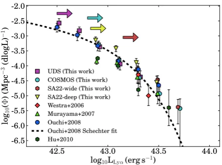
Figure 5.The Lyαluminosity function atz= 5.7 based on dif-ferent fields. For visual reference, a small offset in the luminosities (±0.02 dex) was used to minimize overlapping of points in the fig-ure. The arrows indicate the luminosity bins for which each field has an average completeness higher than 25%. We find significant field to field variations of±0.4 dex in number densities, consistent with results from e.g.Ouchi et al.(2008). We also compare our re-sults per field with previous studies, finding them to be consistent withMurayama et al.(2007) andOuchi et al.(2008). However, by probing larger, multiple volumes we overcome cosmic variance.

following our selection criteria, we also carefully check for any variable sources and/or moving sources which can con-taminate the bright end. Matthee et al. (2015) applied a statistical correction for these potential contaminants, but we chose to investigate sources one by one, following what we do atz = 5.7. We note that such statistical correction works very well for COSMOS and UDS, but is a slight un-derestimation for SA22, as the number of moving sources in SA22 is significantly higher. Nonetheless, we find that none of the results fromMatthee et al.(2016a), which are based on spectroscopic follow-up (Sobral et al. 2015), have signif-icantly changed: luminous LAEs (LLyα >1043.5erg s−1) at z = 6.6 are more common (& 30 times) than previously measured by smaller area studies (e.g.Ouchi et al. 2010). We note that we also apply an aperture correction to the

z= 6.6 LF of +0.11, unchanged fromMatthee et al.(2015).

5 RESULTS

5.1 The z=5.7 Lyαluminosity function

5.1.1 Field to field variations

We group our LAEs in luminosity bins according to their Lyαluminosity. The observed number density in each bin is corrected for its corresponding line-flux completeness cor-rection. We only include sources from sub-fields with a com-pleteness higher than 25%. The number density for each luminosity bin is calculated by multiplying the number of counts by the completeness factor, divided by the probed volume and bin width. The errors are Poissonian, but we add 30% of the completeness correction in quadrature to obtain the final error per bin.

com-puted per field. We find that there is significant scatter, of the order of ±0.4 dex in the number densities, at least for the range of luminosities where we can compare results from all our fields. It may well be that such scatter is reduced for fainter sources, but our sample does not allow us to constrain that as we can only investigate that with a single field (UDS) – seeOuchi et al.(2008). Our results per field are also pre-sented in TableA2. Our results highlight the importance of probing multiple fields and caution the over-interpretation of single field “over” or “under” densities, either in the context of reionization or of structure formation.

5.1.2 Comparison with otherz= 5.7surveys

Several surveys have published LFs ofz= 5.7 LAEs, which we compare with our results (see Figure 5). We compare our results with Westra et al. (2006), Murayama et al. (2007) (COSMOS),Ouchi et al.(2008) (UDS) andHu et al. (2010) (SA22-deep, SSA17, A370 and GOODS-N) in Figure 5. While there are some differences between our selection criteria and the ones applied in these studies, overall we find very good agreement. Moreover, the variance that we see from field to field (see Figure5) is sufficient to explain any subtle differences between our results per field and those in the literature.

For the COSMOS field,Murayama et al.(2007) applies a much more conservative Σ cut (corresponding to roughly Σ > 5) which leads to missing fainter LAEs. The differ-ent Σ cut, together with a differdiffer-ent completeness correc-tion (ours is based on line-flux or luminosity, while

Mu-rayama et al. 2007 does a correction based on detection

completeness) easily explains why our fainter luminosity bin (log10LLyα= 42.9 erg s−1) has a higher number density,

which fully agrees with our UDS and SA22 estimates, along with those presented inOuchi et al.(2008).

Within the errors, our results are also fully consistent with those by Ouchi et al.(2008), at all luminosities. Our brightest bin (log10LLyα= 43.7 erg s−1) is populated only by

our COSMOS and SA22-wide fields, as those have the largest areas (sufficiently large to probe the bright end), but we note that the estimates from COSMOS and SA22-wide fully agree, while we are also in very good agreement with the results fromHu et al.(2010). SA22-deep is both our smallest contiguous field and also the one with the highest number densities (although generally agreeing within the errors with the other fields, particularly given the variance seen). In the SA22-wide field we find number densities consistent with Ouchi et al. (2008) up to log10LLyα = 43.5 erg s−1 and a

brighter bin consistent with our COSMOS number density. The bright end of the Lyα LF seems to point towards a deviation from the Schechter fit presented in Ouchi et al. (2008), better explained by a less accentuated exponential drop, or by a single power-law.

5.1.3 The combinedz= 5.7Lyαluminosity function

We combine our data from the different fields to obtain a combined Lyαluminosity function atz= 5.7. We show the results in Figure6and TableA3.

We fit a Schechter function (Schechter 1976), defined by three parameters: the power-law slopeα, the characteristic number densityφ?_{and the characteristic luminosityL}?_.

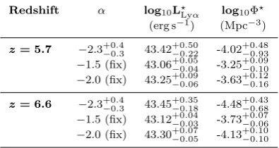
Table 4.Parameters for the best Schechter function fits for the Lyα LFs at z = 5.7 and z = 6.6 (recomputedMatthee et al. 2015). We allowαto vary, but we also fixαto−2.0 and−1.5.

Redshift α log10L?Lyα log10Φ? (erg s−1_{) (Mpc}−3₎

z= 5.7 −2.3+0₋₀._.4₃ 43.42+0_−0..50₂₂ -4.02+0₋₀._.48₉₃

−1.5 (fix) 43.06+0−0..0504 -3.25 +0.09

−0.10

−2.0 (fix) 43.25+0−0..0906 -3.63 +0.12

−0.16

z= 6.6 −2.3+0−0..43 43.45 +0.35

−0.18 -4.48 +0.43

−0.68

−1.5 (fix) 43.12+0−0..0403 -3.73 +0.07

−0.06

−2.0 (fix) 43.30+0_−0..₀₅07 -4.13+0₋₀._.10₁₀

In Table 4, we present best-fit parameters of the Schechter function atz= 5.7. We find the faint end slopeα

to be particularly steep:α=−2.3+0.4

−0.3. This is in very good

agreement with recent results fromDressler et al.(2015) at the same redshift who foundα to be−2.35< α < −1.95 (while we find−2.6< α <−1.9, 1σ). It is therefore clear that the Lyα luminosity function is very steep just after re-ionisation and may be steeper than the UV luminosity function at the same redshift (α≈ −1.9; e.g.Bouwens et al. 2015). Note that such a steep faint-end slope atz = 5.7 is already preferred by the fit inOuchi et al.(2008) and is con-sistent with theoretical expectations (Gronke et al. 2015).

We also fit our LF by fixing the faint-end slope toα=

−2.0 andα=−1.5 and allow Φ?_andL?_{to vary. This allows}

our results to be directly compared with other studies which fixedαto the same values. The results are presented in Table 4.

5.2 Evolution from z=5.7 to z∼7 and beyond

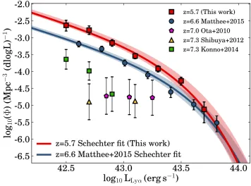
In Section4.5we discuss the steps we took to obtain a com-parable and updatedz= 6.6 Lyαluminosity function, based onMatthee et al.(2015). We show the recomputedz= 6.6 LyαLF, and a comparison with ourz = 5.7 measurement in Figure6. The recomputedz = 6.6 LF is fully presented in TableA3.

We find that both z = 6.6 and z = 5.7 are best fit with a very steep α of ∼ −2.3. At a fixed α, our results show a significant decline in the number density of the more “typical”/faint Lyαemitters fromz = 5.7 to z = 6.6, with

φ∗ declining by 0.5 dex. However, and in very good agree-ment with Matthee et al.(2015), we find little to no evo-lution at the bright end, with L∗ showing no significant evolution, or only a very weak increase of∼0.05−0.1 dex from z = 5.7−6.6 (depending on α). In practice, our re-sults show that the number density of bright Lyα emit-ters (LLyα > 1043.5erg s−1) shows no significant evolution

42.5

43.0

43.5

44.0

log

L

(erg s

)

-6.5

-6.0

-5.5

-5.0

-4.5

-4.0

-3.5

-3.0

-2.5

-2.0

log

10

(

Φ

)(Mpc

−

3

(dlogL)

−

1

)

z=5.7 Schechter fit (This work)

z=6.6 Matthee+2015 Schechter fit

z=5.7 (This work) z=6.6 Matthee+2015 z=7.0 Ota+2010 z=7.3 Shibuya+2012 z=7.3 Konno+2014

Figure 6. Evolution of the Lyα LF fromz= 5.7 toz= 6.6. Thez= 6.6 LF is our updated version fromMatthee et al.(2015), see Section 4.5. The colored regions around the best Schechter fit show the 1σ error inL∗_{. We observe a strong decrease in the number}

density of the fainter LAEs as we increase with redshift up toz= 6.6 and alsoz >7 (Ota et al. 2010;Shibuya et al. 2012;Konno et al. 2014). This decrease can likely be explained by a more neutral IGM as we go deeper into the reionization epoch. However, there seems to be no evolution for the brighter sources, which can likely be explained by a preferential reionization around the brightest sources. There is currently a lack of comparable surveys atz >7 at the brightest luminosities.

that may explain how these sources have been able to likely reionize their surroundings already atz∼7. Further obser-vations will be able to confirm a larger, statistical sample at

z ∼7, but our new sample atz= 5.7 is uniquely suited to be directly compared.

Figure6also presents results from severalz >7 narrow band surveys from the literature, which we compare with

z = 6.6 andz = 5.7. The trend that we see fromz = 5.7 to z = 6.6 of significant decrease in the number density of faint Lyαemitters seems to continue at a fast pace toz∼7 and beyond (Ota et al. 2010; Shibuya et al. 2012; Konno et al. 2014). We provide a more detailed discussion about the differential evolution of the Lyαas an imprint of reionization in Section6. There is currently a lack of comparable surveys atz >7 at the brightest luminosities, so it is not yet possible to test whether the lack of evolution at the bright end still holds atz >7.

5.3 The Lyαsizes and evolution at z=5.7−6.6

Since the Lyαtransition is resonant, Lyα photons scatter in a medium with neutral hydrogen. Because of this, Lyα

photons tend to escape over much large radii than their UV and Hαcounterparts, making them observable as Lyαhaloes (e.g. Rauch et al. 2008; Steidel et al. 2011; Momose et al. 2014;Matthee et al. 2016a). Therefore, the aperture that is used to measure Lyαis critical (e.g. Wisotzki et al. 2016). Typically, LAE surveys have attempted to take extended

Lyα emission into account by using _mag-auto measure-ments (e.g.Ouchi et al. 2010;Konno et al. 2016) or relatively large apertures (e.g.Murayama et al. 2007;Hu et al. 2010, who use 300apertures atz = 5.7). However, the total mea-sured magnitude with_mag-auto depends on the depth of the narrow-band imaging, such that a comparison between surveys and redshifts is challenging, particularly asWisotzki et al.(2016) show that Lyαextends well beyond the typical limiting surface brightness of narrow-band surveys.

While we use fixed 200apertures in similar excellent see-ing conditions at bothz = 5.7 andz = 6.6 (as this allows to understand the completeness and selection function in an optimal way; c.f. Matthee et al. 2015), we correct for any flux missed as described in Section4.3.

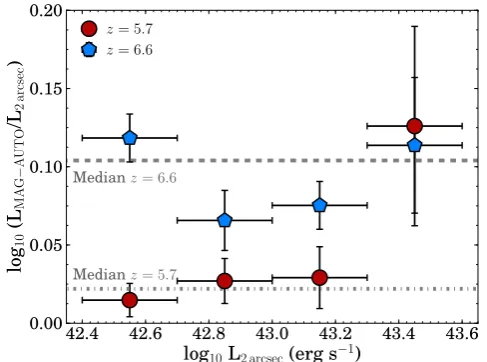
Matthee et al.(2015) found that 200apertures systemat-ically underestimate Lyαluminosities atz= 6.6 (compared to the_mag-auto) with a median offset of 0.11 dex over the spectroscopically confirmed sample of LAEs (confirmed in Ouchi et al. 2010). Here we extend this analysis to the full sample of sources at bothz= 5.7 andz= 6.6. We find that the median offset between the_mag-autoluminosity and the 200aperture offset atz= 6.6 is 0.11 dex, while it is only 0.02 dex atz = 5.7; see Figure 7. The latter explains why our 200measurements result in very similar number densities as literature studies with larger apertures atz = 5.7, see Fig. 5.

in-42.4 42.6 42.8 43.0 43.2 43.4 43.6

log10L2 arcsec(erg s−1)

0.00 0.05 0.10 0.15 0.20

log

10

(LMA

G

−

A

UTO

/L2

arcsec

)

Medianz= 6.6

Medianz= 5.7

z= 5.7

z= 6.6

Figure 7. The median difference inmag-auto luminosity and luminosity within 200 apertures in bins of the 200 aperture Lyα luminosity for LAE samples atz= 5.7 andz= 6.6. The dashed and dashed-dotted grey lines indicate the median of all LAEs in the sample, which is obviously dominated by low luminosity sources. At both redshifts, more centrally luminous LAEs also have relatively more flux at larger radii (which is captured by

mag-auto). At faint central luminosities LAEs atz= 6.6 appear

more extended, which could be due to increased scattering in HI around galaxies. We note that this may be one of the causes for the apparent evolution in the LyαLF, and may also be important to consider when interpreting the spectroscopic follow-up of UV-selected galaxies with low Lyα luminosities, as slits will recover even less of the total flux.

creases slightly with increasing Lyαluminosity (see Fig.7). Specifically, the most luminous LAEs have larger Lyαhaloes (and more flux at larger radii) than the typical fainter ones. Interestingly, we find a different behaviour atz= 6.6. While the brightestz= 6.6 Lyαseem to be as extended as those at

z= 5.7 (these are the ones that may have already been able to fully ionise the surrounding environment), fainter Lyα

emitters atz = 6.6 are all more extended than comparable sources atz= 5.7. Together with the differential evolution of the LyαLF, our results provide strong evidence for reion-ization effects being much stronger for the faint sources than for the bright ones. We discuss this trend further in Section 6.

A similar but more careful analysis of the extent of Lyα

emission atz = 5.7−6.6 than our own has been done by Momose et al.(2014), who created stacked narrow band and broad band images of the LAEs in UDS fromOuchi et al. (2008, 2010). They observed that Lyα is extended, being more extended than their UV counterpart (while also being more extended than the PSF of their images; a similar trend is found for individual LAEs by e.g. Wisotzki et al. 2016).

Momose et al. 2014 found evidence of an increase in the

scale length of Lyαfromz = 5.7 toz= 6.6. However, they did not separate their sample in bins of luminosity and their results are obtained with median stacking. This means that the faintest sources dominate (as there are more faint sources than luminous ones) and that these results are more repre-sentative of a “typical” LAE, with LLyα ∼ 1042.6erg s−1.

The median evolution in the scale length of Lyα haloes from LAEs estimated inMomose et al.(2014) is thus consis-tent with the difference between_mag-autoand 200 measure-ments that we find for relatively faint LAEs betweenz= 5.7 andz= 6.6.

6 DISCUSSION: IMPRINTS FROM REIONIZATION?

As noted before, the observed Lyα luminosity at a fixed spatial scale is expected to decrease in the reionization era, as an increasingly neutral IGM scatters Lyαphotons into larger, extended haloes (e.g.Dijkstra 2014). Our results are consistent with witnessing such predictions directly. Here we discuss the differences we observe in the Lyαluminosity function betweenz= 5.7 andz= 6.6, and also our results on the extent of Lyαemitters atz= 5.7 andz= 6.6. For earlier work, see e.g.Dijkstra et al.(2007),Ouchi et al.(2010) and Hu et al.(2010).

We observe strong differential evolution of the LyαLF fromz∼6 toz∼7, with a significant decrease (−0.5 dex) in the number density for Lyαluminosities belowL∗. The drop in the observability of faint LAEs may well be explained by a larger fraction of neutral IGM atz >6 caused by reioniza-tion not being completed. The brightest emitters would not suffer from such a decline because their strong Lyαemission is easier to be observed, as previously illustrated by the sim-ple toy model inMatthee et al.(2015). This model assumes that the Lyαluminosity scales with the ionising output and LAEs are only observed if they are either capable of ionising the IGM around them, or are strongly clustered. To first or-der, a stronger ionising output for brighter LAEs is expected because Lyαis a recombination line (such that at fixed es-cape fraction, a higher Lyαluminosity scales with the num-ber of ionising photons). Also, as shown in Matthee et al. (2016b), LAEs at z = 2.2 typically produce more ionising photons per unit UV luminosity than more typical galaxies such as Hαemitters (HAEs). Furthermore, as hypothesised byDijkstra & Gronke (2016), ISM conditions which favor the escape of Lyαphotons also likely favor the escape of Ly-man continuum (LyC) photons (for example due to a porous ISM), such that in addition to producing more ionising pho-tons, LAEs could also leak more ionising photons into the IGM.

Recent evidence fromStark et al.(2016) shows that the fraction of bright UV selected galaxies (LBGs) with strong Lyαemission is much higher than was previously found (e.g. Schenker et al. 2014; Pentericci et al. 2014; Schmidt et al. 2016) when they are selected on strong nebular lines (e.g. Hβ/[O_iii]). This is likely because UV-bright galaxies are in over-dense regions and emit copious amount of ionising ra-diation (inferred from observed high ionization UV lines as Ciii] and their high EW optical nebular lines). Such con-ditions may also favor the production of Lyαphotons and lead to larger ionised bubbles. Therefore, these observations are in principle consistent with the observed evolution of the LyαLF, where we observe reionization completing first around luminous LAEs.

be connected to the neutral fraction of the IGM (e.g. Dijk-stra & Loeb 2008). As we show in Figure 7, we find that the median difference between 200 apertures and the total magnitude (as observed withmag-auto) is much smaller at

z= 5.7 than atz= 6.6. Most interestingly, the major differ-ence is found at the faintest luminosities. Atz= 6.6, LAEs which have a low central luminosity have a relatively much larger total luminosity than atz= 5.7. This means that at a fixed surface brightness limit (note that the limiting sur-face brightness at z = 6.6 is actually even slightly higher), faint LAEs are more extended atz= 6.6 than atz= 5.7. For more luminous LAEs the difference is much smaller. This ef-fect can easily be explained in the framework of theMatthee et al.(2015) toy-model: faint LAEs are surrounded by a rel-atively more neutral IGM, such that there is more resonant scattering leading to more extended emission.

The evolution of the LyαLF and the extent of Lyαfor different luminosities may very well be explained by a patchy reionization scenario where the IGM is ionised first around luminous LAEs. However, internal effects from galaxies may also be important. Furthermore, studying the clustering of both bright and faint LAEs and how it evolves from e.g.

z = 5.7 to z = 6.6 and beyond (e.g. Mesinger 2010;Ouchi et al. 2010) will provide the extra, necessary constraints. A similar analysis with future larger samples of LAEs (for example from the Hyper Suprime Cam survey) will be very useful to confirm the observed trends.

Our results also mean that a careful approach is re-quired in order to interpret the observed Lyα fraction for samples of LBGs at different redshifts in terms of a vary-ing neutral fraction due to reionization, because different samples of LBGs show very different Lyαfractions. Curtis-Lake et al.(2012) found a remarkably high fraction of strong LAEs amongst luminous LBGs,Stark et al.(2016) found a higher Lyα fraction for LBGs selected on strong nebular emission and Erb et al. (2016) found that z ∼ 2 galaxies with extreme line ratios have high Lyαfractions. Moreover, our results show that typical, faint Lyα emitters become more extended as we go into the reionization epoch, with the same (or even less) flux being spread over larger areas. This is an additional challenge for the traditional slit spec-troscopy follow-up, which will struggle to detect any Lyαif the flux is significantly extended.

7 CONCLUSIONS

We have constructed the largest Lyα narrow band survey atz= 5.7, when re-ionization is close to complete. We have surveyed a total area of 7 deg2and a volume of 6.3×106Mpc3 at z = 5.7, covering the COSMOS, UDS and SA22 fields. Here we summarize the main conclusions:

• By identifying strong line-emitters with a Lyman break, we find 514 LAE candidates at z = 5.7 with EW0 >25 ˚A

(EW0∼25−1000 ˚A) and luminosities ranging from 1042.5−

1044erg s−1, in a single, homogeneous data-set.

• We find that cosmic variance plays a major role, with variations of ±0.4 dex in number densities of Lyα emitters from field to field.

• By combining all our fields and overcoming cosmic vari-ance, we find that the faint end slope of the z = 5.7 Lyα

luminosity function is very steep, with α = −2.3+0−0..43. If

we fix α = −2.0, we find L? = 1043.22+0−0..0805_{erg s}−1 _and

Φ?=−3.60+0−0..1216Mpc

−3

.

• We also present an updated z = 6.6 Lyα luminosity function, based on comparable volumes, and obtained with the same methods, which we directly compare with that at

z= 5.7.

• We find significant evolution from z = 5.7 (after re-ionization) to z = 6.6 (within the epoch of re-ionization) at the faint end. We find that the fainter the luminosity, the stronger the drop in the number density of Lyα emit-ters. The strong decrease of the number density of faint Lyα

emitters continues toz∼7.

• At bright Lyα luminosities (LLyα >1043.5erg s−1) we

find no evolution in the number density of Lyα emitters when we enter the re-ionization era. This is consistent with bright Lyαemitters being preferentially observable because they already are in ionized bubbles even atz∼7.

• Faint Lyα emitters at z = 6.6 show more extended haloes than those atz= 5.7, suggesting that neutral Hydro-gen plays a more important role of scattering Lyαphotons atz= 6.6.

All together, our results indicate that we are observing patchy reionization happening first around the brightest Lyα

emitters, allowing the number densities of those sources to remain unaffected by the increase of neutral Hydrogen from

z ∼5 toz ∼7. We observe a preferential evolution of the faint end of the LyαLF fromz = 5.7 toz = 6.6. There is a decrease in the faint end while the bright end shows little to no evolution. We also observe no evolution in the sizes of the brighter emitters, which could be interpreted as showing no evidence of extra scattering around them fromz = 5.7 toz= 6.6, while faint sources show a significant difference, presenting much more flux at larger radii, which could be explained by faint LAEs being located in a more neutral IGM leading to more resonant scattering and extended emis-sion. The spectroscopic confirmation of relatively bright Lyα

emitters beyondz∼7 and approachingz∼9 (Oesch et al. 2015; Zitrin et al. 2015) may already be hinting that our results may hold to even higher redshifts.

The nature and diversity of bright Lyα sources at

z = 6.6, which we find to have essentially the same num-ber density as those atz= 5.7, are starting to be unveiled. Spectroscopic follow up (e.g.Ouchi et al. 2013;Sobral et al. 2015; Zabl et al. 2015;Hu et al. 2016), detailed modelling (e.g.Hartwig et al. 2015;Dijkstra et al. 2016;Agarwal et al. 2016;Visbal et al. 2016;Smidt et al. 2016;Smith et al. 2016) and other observations with HST and ALMA (Ouchi et al. 2013;Sobral et al. 2015;Schaerer et al. 2015;Bowler et al. 2016) are revealing a surprising diversity. Current results indicate that these sources may have a range of powering sources (from metal poor populations to multiple stellar pop-ulations and also AGN, including potentially direct collapse black holes). Regardless of their nature, their observabil-ity requires the production and emission of the necessary amount of ionising LyC photons capable of ionising a large enough local bubble to make them observable as bright Lyα

observations of our sample of bright z = 5.7 sources and of much larger, statistical samples at z ∼ 5−7 will cer-tainly shed light over many of the current open questions, while the availability of JWST will provide a revolutionary window into the physical conditions within these sources.

ACKNOWLEDGEMENTS

We thank the anonymous referee for useful and construc-tive comments and suggestions which greatly improved the quality and clarity of our work. The authors ac-knowledge financial support from the Netherlands Or-ganisation for Scientific research (NWO) through a Veni fellowship. SS and DS acknowledge funding from FCT through a FCT Investigator Starting Grant and Start-up Grant (IF/01154/2012/CP0189/CT0010). SS also ac-knowledges support from FCT through the research grants UID/FIS/04434/2013 and PTDC/FIS-AST/2194/2012. JM acknowledges a Huygens PhD fellowship from Leiden Uni-versity.

Based on observations with the Subaru Telescope (Pro-gram IDs: S05B-027, S06A-025, S06B-010, S07A-013, S07B-008, S08B-S07B-008, S09A-017, S14A-086). Based on observations made with ESO Telescopes at the La Silla Paranal Obser-vatory under programme ID 294.A-5018. Based on observa-tions obtained with MegaPrime/Megacam, a joint project of CFHT and CEA/IRFU, at the Canada-France-Hawaii Tele-scope (CFHT) which is operated by the National Research Council (NRC) of Canada, the Institut National des Science de l’Univers of the Centre National de la Recherche Scien-tifique (CNRS) of France, and the University of Hawaii. This work is based in part on data products produced at Ter-apix available at the Canadian Astronomy Data Centre as part of the Canada-France-Hawaii Telescope Legacy Survey, a collaborative project of NRC and CNRS. Based on data products from observations made with ESO Telescopes at the La Silla Paranal Observatory under ESO programme ID 179.A-2005 and on data products produced by TERAPIX and the Cambridge Astronomy Survey Unit on behalf of the UltraVISTA consortium. We are grateful to the CFHTLS, COSMOS-UltraVISTA, UKIDSS, SXDF and COSMOS sur-vey teams. Without these legacy sursur-veys, this research would have been impossible.

The authors wish to recognize and acknowledge the very significant cultural role and reverence that the summit of Mauna Kea has always had within the indigenous Hawaiian community. We are most fortunate to have the opportunity to conduct and explore observations from this mountain.

Finally, the authors acknowledge the unique value of the publicly available programming language Python, includ-ing the numpy,pyfits, matplotlib, scipyand astropy

(Astropy Collaboration et al. 2013) packages.

REFERENCES

Adams J. J., et al., 2011,ApJS,192, 5

Agarwal B., Johnson J. L., Zackrisson E., Labbe I., van den Bosch F. C., Natarajan P., Khochfar S., 2016,MNRAS,

Astropy Collaboration et al., 2013,A&A,558, A33 Bacon R., et al., 2015,AAP,575, A75

Bayliss M. B., Wuyts E., Sharon K., Gladders M. D., Hennawi J. F., Koester B. P., Dahle H., 2010,ApJ,720, 1559 Becker G. D., Bolton J. S., Madau P., Pettini M., Ryan-Weber

E. V., Venemans B. P., 2015,MNRAS,447, 3402

Bertin E., 2006, in Gabriel C., Arviset C., Ponz D., Enrique S., eds, Astronomical Society of the Pacific Conference Series Vol. 351, Astronomical Data Analysis Software and Systems XV. p. 112

Bertin E., Arnouts S., 1996,AAPS,117, 393

Bertin E., Mellier Y., Radovich M., Missonnier G., Didelon P., Morin B., 2002, in Bohlender D. A., Durand D., Handley T. H., eds, Astronomical Society of the Pacific Conference Se-ries Vol. 281, Astronomical Data Analysis Software and Sys-tems XI. p. 228

Blanc G. A., et al., 2011,ApJ,736, 31

Borisova E., et al., 2016, preprint, (arXiv:1605.01422)

Boulade O., et al., 2003, in Iye M., Moorwood A. F. M., eds, Proc. SPIEVol. 4841, Instrument Design and Perfor-mance for Optical/Infrared Ground-based Telescopes. pp 72– 81,doi:10.1117/12.459890

Bouwens R. J., et al., 2015,ApJ,803, 34

Bowler R. A. A., Dunlop J. S., McLure R. J., McLeod D. J., 2016, preprint, (arXiv:1605.05325)

Bunker A. J., Warren S. J., Hewett P. C., Clements D. L., 1995, MNRAS,273, 513

Capak P., et al., 2007,ApJS,172, 99 Capak P. L., et al., 2015,Nature,522, 455

Caruana J., Bunker A. J., Wilkins S. M., Stanway E. R., Lacy M., Jarvis M. J., Lorenzoni S., Hickey S., 2012,MNRAS,427, 3055

Caruana J., Bunker A. J., Wilkins S. M., Stanway E. R., Loren-zoni S., Jarvis M. J., Ebert H., 2014,MNRAS,443, 2831 Casali M., et al., 2007,A&A,467, 777

Cassata P., et al., 2011,A&A,525, A143 Cassata P., et al., 2015,A&A,573, A24 Castellano M., et al., 2016,ApJ,818, L3 Cirasuolo M., et al., 2007,MNRAS,380, 585 Cowie L. L., Hu E. M., 1998,AJ,115, 1319 Curtis-Lake E., et al., 2012,MNRAS,422, 1425

Dijkstra M., 2014,Publ. Astron. Soc. Australia,31, e040 Dijkstra M., Gronke M., 2016, preprint, (arXiv:1604.08208) Dijkstra M., Loeb A., 2008,MNRAS,386, 492

Dijkstra M., Lidz A., Wyithe J. S. B., 2007,MNRAS,377, 1175 Dijkstra M., Gronke M., Sobral D., 2016,ApJ,823, 74

Dressler A., Henry A., Martin C. L., Sawicki M., McCarthy P., Villaneuva E., 2015,ApJ,806, 19

Dunlop J. S., McLure R. J., Robertson B. E., Ellis R. S., Stark D. P., Cirasuolo M., de Ravel L., 2012,MNRAS,420, 901 Dunlop J. S., et al., 2016, preprint, (arXiv:1606.00227) Erb D. K., Pettini M., Steidel C. C., Strom A. L., Rudie G. C.,

Trainor R. F., Shapley A. E., Reddy N. A., 2016, preprint, (arXiv:1605.04919)

Fan X., et al., 2006,ApJ,132, 117 Finkelstein S. L., et al., 2015,ApJ,810, 71 Fontana A., et al., 2010,ApJ,725, L205 Furusawa H., et al., 2008,ApJS,176, 1

Gronke M., Dijkstra M., Trenti M., Wyithe S., 2015,MNRAS, 449, 1284

Hartwig T., et al., 2015, preprint, (arXiv:1512.01111) Hayes M., Schaerer D., ¨Ostlin G., 2010,AAP,509, L5

Hayes M., Schaerer D., ¨Ostlin G., Mas-Hesse J. M., Atek H., Kunth D., 2011,ApJ,730, 8

Hu E. M., Cowie L. L., Barger A. J., Capak P., Kakazu Y., Trouille L., 2010,ApJ,725, 394

Hu E. M., Cowie L. L., Songaila A., Barger A. J., Rosenwasser B., Wold I., 2016, preprint, (arXiv:1606.03526)

Kashikawa N., et al., 2011,ApJ,734, 119

Khostovan A. A., Sobral D., Mobasher B., Best P. N., Smail I., Stott J. P., Hemmati S., Nayyeri H., 2015,MNRAS,452, 3948 Khostovan A. A., Sobral D., Mobasher B., Smail I., Darvish B., Nayyeri H., Hemmati S., Stott J. P., 2016, preprint, (arXiv:1604.02456)

Kim J.-W., Im M., Lee S.-K., Edge A. C., Wake D. A., Merson A. I., Jeon Y., 2015,ApJ,806, 189

Konno A., et al., 2014,ApJ,797, 16

Konno A., Ouchi M., Nakajima K., Duval F., Kusakabe H., Ono Y., Shimasaku K., 2016,ApJ,823, 20

Laigle C., et al., 2016, preprint, (arXiv:1604.02350) Lawrence A., et al., 2007,MNRAS,379, 1599 Ly C., et al., 2007,ApJ,657, 738

Ly C., Lee J. C., Dale D. A., Momcheva I., Salim S., Staudaher S., Moore C. A., Finn R., 2011,ApJ,726, 109

Madau P., 1995,ApJ,441, 18

Madau P., Dickinson M., 2014,ARAA,52, 415 Maiolino R., et al., 2015,MNRAS,452, 54 Malhotra S., Rhoads J. E., 2004,ApJL,617, L5 Mallery R. P., et al., 2012,ApJ,760, 128 Martin C. L., Sawicki M., 2004,ApJ,603, 414 Matthee J. J. A., et al., 2014,MNRAS,440, 2375

Matthee J., Sobral D., Santos S., R¨ottgering H., Darvish B., Mobasher B., 2015,MNRAS,451, 400

Matthee J., Sobral D., Oteo I., Best P., Smail I., R¨ottgering H., Paulino-Afonso A., 2016a,MNRAS,

Matthee J., Sobral D., Best P., Khostovan A. A., Oteo I., Bouwens R., R¨ottgering H., 2016b, preprint, (arXiv:1605.08782) McCracken H. J., et al., 2012,A&A,544, A156

Mesinger A., 2010,MNRAS,407, 1328 Miyazaki S., et al., 2002,PASJ,54, 833 Momose R., et al., 2014,MNRAS,442, 110 Murayama T., et al., 2007,ApJs,172, 523 Nilsson K. K., et al., 2007,A&A,471, 71 Oesch P. A., et al., 2015,ApJ,804, L30 Ono Y., et al., 2012,ApJ,744, 83 Ota K., et al., 2010,ApJ,722, 803 Ouchi M., et al., 2004,ApJ,611, 660 Ouchi M., et al., 2008,ApJs,176, 301 Ouchi M., et al., 2010,ApJ,723, 869 Ouchi M., et al., 2013,ApJ,778, 102

Partridge R. B., Peebles P. J. E., 1967,ApJ,147, 868 Pentericci L., et al., 2014,ApJ,793, 113

Pritchet C. J., 1994,PASP,106, 1052 Rauch M., et al., 2008,ApJ,681, 856

Rhoads J. E., Malhotra S., Dey A., Stern D., Spinrad H., Jannuzi B. T., 2000,ApJL,545, L85

Rhoads J. E., et al., 2003,AJ,125, 1006

Robertson B. E., Ellis R. S., Dunlop J. S., McLure R. J., Stark D. P., 2010,Nature,468, 49

Sawicki M., et al., 2008,ApJ,687, 884

Schaerer D., Boone F., Zamojski M., Staguhn J., Dessauges-Zavadsky M., Finkelstein S., Combes F., 2015, A&A, 574, A19

Schechter P., 1976,ApJ,203, 297

Schenker M. A., Stark D. P., Ellis R. S., Robertson B. E., Dunlop J. S., McLure R. J., Kneib J.-P., Richard J., 2012,ApJ,744, 179

Schenker M. A., Ellis R. S., Konidaris N. P., Stark D. P., 2014, ApJ,795, 20

Schmidt K. B., et al., 2016,ApJ,818, 38

Shibuya T., Kashikawa N., Ota K., Iye M., Ouchi M., Furusawa H., Shimasaku K., Hattori T., 2012,ApJ,752, 114

Shimasaku K., et al., 2006,PASJ,58, 313 Skrutskie M. F., et al., 2006,AJ,131, 1163

Smidt J., Wiggins B. K., Johnson J. L., 2016, preprint, (arXiv:1603.00888)

Smith A., Bromm V., Loeb A., 2016, preprint, (arXiv:1602.07639)

Sobral D., et al., 2009,MNRAS,398, L68

Sobral D., Smail I., Best P. N., Geach J. E., Matsuda Y., Stott J. P., Cirasuolo M., Kurk J., 2013,MNRAS,428, 1128 Sobral D., Matthee J., Darvish B., Schaerer D., Mobasher B.,

R¨ottgering H. J. A., Santos S., Hemmati S., 2015,ApJ,808, 139

Stark D. P., Ellis R. S., Richard J., Kneib J.-P., Smith G. P., Santos M. R., 2007,ApJj,663, 10

Stark D. P., Ellis R. S., Chiu K., Ouchi M., Bunker A., 2010, MNRAS,408, 1628

Stark D. P., et al., 2016, preprint, (arXiv:1606.01304) Steidel C. C., Bogosavljevi´c M., Shapley A. E., Kollmeier J. A.,

Reddy N. A., Erb D. K., Pettini M., 2011,ApJ,736, 160 Taniguchi Y., et al., 2005,PASJ,57, 165

Taniguchi Y., et al., 2007,ApJS,172, 9

Taylor M. B., 2006, in Gabriel C., Arviset C., Ponz D., Enrique S., eds, Astronomical Society of the Pacific Conference Series Vol. 351, Astronomical Data Analysis Software and Systems XV. p. 666

Visbal E., Haiman Z., Bryan G. L., 2016,MNRAS, Warren S. J., et al., 2007, arXiv:0703037,

Watson D., Christensen L., Knudsen K. K., Richard J., Gallazzi A., Micha lowski M. J., 2015,Nature,519, 327

Westra E., et al., 2006,AAP,455, 61 Wisotzki L., et al., 2016,A&A,587, A98

Zabl J., Nørgaard-Nielsen H. U., Fynbo J. P. U., Laursen P., Ouchi M., Kjærgaard P., 2015,MNRAS,451, 2050

Zitrin A., et al., 2015,ApJ,810, L12

van Breukelen C., Jarvis M. J., Venemans B. P., 2005,MNRAS, 359, 895

APPENDIX A: FILTER PROFILE CORRECTIONS AND LFS

FigureA1shows the effect of our filter profile corrections. We show the completeness corrected number densities of LAEs in bins of Lyα luminosity for individual fields at z = 5.7 (TableA2) and for the combined coverage at z = 5.7 and

z= 6.6 (TableA3).

Table A1.For each field we present the median line-flux completeness per bin, which we use to correct thez= 5.7 number densities. We only consider number densities from sub-fields with a line-flux completeness higher than 25%.

Luminosity bins Line-flux completeness

log10L [erg s−1] Percentage [%]

(UDS) (COSMOS) (SA22-deep) (SA22-wide)

42.5±0.1 27 <25 <25 <25

42.7±0.1 30 <25 <25 <25

42.9±0.1 45 37 36 <25

43.1±0.1 53 54 56 <25

43.3±0.1 61 65 68 51

43.5±0.1 73 73 77 63

43.7±0.1 83 80 84 74

42.5 43.0 43.5 44.0

log10LLyα(erg s−1) -6.5

-6.0 -5.5 -5.0 -4.5 -4.0 -3.5 -3.0 -2.5 -2.0

log

10

(

Φ

)(Mpc

−

3(dlogL)

−

1)

UDS+COSMOS+SA22 (This work) Schechter fit (This work)

UDS+COSMOS+SA22 filter corrected (This work) Filter corrected Schechter fit (This work) Ouchi+2008

Our Schechter fit to Ouchi+2008

Figure A1.The number densities in luminosity bins from our survey in the UDS, COSMOS and SA22 fields (red squares) and the bins from Ouchi et al.(2008) in blue triangles. A small lu-minosity correction of +0.02 was applied to our lulu-minosity bins to correct for extended emission (this correction is discussed in

§5.3). The Schechter fits to the luminosity bins from our study agrees very well withOuchi et al.(2008). In green we also show the luminosity bins from this work after we apply a filter profile bias correction (we estimate this correction in§4.2) and the cor-rected LF Schechter fit. The effect of this correction is strongest at the brightest bins.

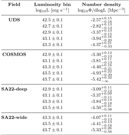
Table A2.The completeness corrected number density of LAEs in the different surveyed fields atz= 5.7.

Field Luminosity bin Number density log10L [erg s−1] log10Φ/dlogL [Mpc−3]

UDS 42.5±0.1 -2.57+0₋₀._.15₁₆ 42.7±0.1 -2.82+0−0..1313 42.9±0.1 -3.37+0−0..1315 43.1±0.1 -3.94+0−0..1620 43.3±0.1 -4.37+0₋₀._.21₃₃ COSMOS 42.9±0.1 -3.30+0₋₀._.12₁₃ 43.1±0.1 -3.81+0₋₀._.11₁₃ 43.3±0.1 -4.40+0−0..1621 43.5±0.1 -4.93+0−0..2239 43.7±0.1 -5.42+0−∞.32

Table A3.The completeness and filter profile bias corrected luminosity functions atz= 5.7 andz= 6.6 from this study. Note that we corrected the bins for extended emission (see Section5.3).

Redshift Luminosity bin Volume Observed number density Corrected number density log10L [erg s−1] [106Mpc3] log10Φ/dlogL [Mpc−3] log10Φ/dlogL [Mpc−3]

z= 5.7 42.52±0.1 0.19 -3.16₋+0₀._.08₀₉ -2.63+0₋₀._.16₁₇ 42.72±0.1 0.65 -3.32+0₋₀._.05₀₆ -2.77+0₋₀._.12₁₃

42.92±0.1 3.09 -3.65+0−0..0404 -3.15

+0.10

−0.10

43.12±0.1 3.09 -3.89+0−0..0505 -3.54

+0.08

−0.08

43.32±0.1 6.30 -4.34+0−0..0506 -3.91

+0.09

−0.10 43.52±0.1 6.30 -4.70+0₋₀._.08₁₀ -4.27+0₋₀._.11₁₂ 43.72±0.1 6.30 -5.62+0₋₀._.20₃₇ -5.12+0₋₀._.22₄₀ z= 6.6 42.61±0.1 0.38 -3.46₋+0₀._.09₀₈ -3.18+0₋₀._.08₀₉ 42.81±0.1 0.64 -3.59+0₋₀._.08₀₇ -3.32+0₋₀._.08₀₈

43.01±0.1 1.07 -4.01+0−0..1109 -3.74

+0.09

−0.10

43.21±0.1 1.73 -4.42+0−0..1411 -4.10

+0.10

−0.11

43.41±0.1 1.73 -4.94+0−0..3018 -4.60

+0.14