Contests on Networks

Economics Working Paper Series

2017/006

Contests on Networks

Alexander Matros and David Rietzke

The Department of Economics Lancaster University Management School

Lancaster LA1 4YX UK

© Authors

All rights reserved. Short sections of text, not to exceed two paragraphs, may be quoted without explicit permission,

provided that full acknowledgement is given.

Contests on Networks

Alexander Matros

David Rietzke

February 24, 2017

Abstract

We develop a model of contests on networks. Each player is “connected” to a set of contests, and exerts a single effort to increase the probability of winning each contest to which she is connected. We characterize equilibria under both the Tullock and all-pay auction contest success functions (CSFs), and show that many well-known results from the contest literature can be obtained by varying the struc-ture of the network. We also obtain a new exclusion result: We show that, under both CSFs, equilibrium total effort may be higher when one player is excluded from the network. This finding contrasts the existing literature, which limits find-ings of this sort to the all-pay auction CSF. Our framework has a broad range of applications, including research and development, advertising, and research funding.

Keywords: Network Games, Contests, Bipartite Graph, Tullock Contest, All-pay Auction

JEL Classifications: C72, D70, D85

∗_{Moore School of Business, University of South Carolina and Lancaster University Management}

School.

1

Introduction

In recent years, economists have recognized the importance of understanding how the structure of interactions affects economic behavior, which has led to the development of research on networks. The importance of this field of research is unquestionable, due to the broad applicability of these models in many economically relevant settings; to name a few: job search and employment dynamics (Armengol and Jackson, 2004; Calv´o-Armengol, 2004), the provision of public goods (Bramoull´e and Kranton, 2007; Bramoull´e et al., 2014), collaboration/research and development (Goyal and Moraga-Gonzalez, 2001; Goyal and Joshi, 2003), and criminal activity (Calv´o-Armengol and Zenou, 2004; Ballester et al., 2006). Jackson and Zenou (2014) provide a comprehensive overview of the literature on network games, and emphasize three approaches researchers have taken to study such games:1 _{(1) games of strategic complements and substitutes; (2) games with linear}

best-replies; and (3) settings with an uncertain pattern of interactions.2 _{These three approaches}

have proved fruitful in allowing researchers to understand how the underlying pattern of interactions affects behavior.

In this paper, we study a new class of network games: contests on networks. Our model consists of a set of players and a set of contests, which form a commonly known bipartite graph (or network).3 _{Each player competes in contests to which she is connected}

by exerting a single effort. A player’s expected payoff depends on her own effort, and the efforts of her competitors. Contests can be used to model many economically relevant situations, and there is a vast literature that analyzes individual and aggregate behavior.4

Our interest here is to understand how the pattern of interactions affects behavior. Our model has a number of interesting applications including, for example, central-ized R&D decisions by multinational firms (MNFs). Prizes are commonly used tools to encourage R&D activity,5 _{and contests can be used to model both explicit R&D contests}

or patent races (e.g. Che and Gale, 2003; Baye and Hoppe, 2003). To take advantage of economies of scale and scope, historically, R&D activity within MNFs has tended to be

1_{See also Jackson (2008) and Bramoull´e and Kranton (2016).}

2_{Examples of models with an uncertain pattern of interactions include Jackson and Yariv (2007),}

Galeotti et al. (2010)

3_{A bipartite graph is a graph in which the vertices may be partitioned into two disjoint subsets, and}

the edges connect the vertices from these subsets.

4_{For relevant surveys see Nitzan (1994), Congleton et al. (2008), and Konrad (2009).}

5_{Innovation prizes were a central feature of the Obama Administration’s efforts to stimulate American}

centralized, and undertaken at the corporate level (Gassmann and Von Zedtwitz, 1999). In this interpretation, the firm chooses a single level of R&D effort, the benefits of which are then realized by each branch of the firm. Our model could also be interpreted in the context of a national advertising campaign by a geographically dispersed franchised firm. In this context, each firm chooses a level of expenditure on a national advertising cam-paign, which increases the share of the market each franchise expects to capture. Finally, one might also interpret our model in the context of research funding. In this setting, researchers exert effort on a project proposal, which they then submit to various funding agencies to increase their chances of receiving funding for their project.

The main contributions of this research are twofold. First, we contribute to the litera-ture on networks by analyzing a new class of network games. We characterize equilibrium behavior in terms of the underlying network characteristics, and study how these char-acteristics influence behavior. Second, we contribute to the literature on contests by establishing connections between several important observations in the contest literature, and different network structures in our setting. That is, we provide a unified framework, within which many well-known results in the contest literature can be obtained by simply varying the structure of the network. We also explore how equilibrium behavior depends on the contest success function (CSF), focusing on the two most widely used CSFs in the contest literature – the Tullock CSF, and the all-pay auction (APA) CSF.6

We show that the equilibrium behavior in symmetric contests7 _{– a contest in which}

players compete for a single prize of common value – is analogous to equilibrium behavior (for both CSFs) in our model, when the network is biregular.8 _{We also show that}

equi-librium behavior depends only on player and prize degrees, and is independent from the number of players and the number of prizes. Consistent with well-known results, when the network is biregular, total equilibrium effort is always higher under the APA CSF than under the Tullock CSF.

We then show that equilibrium behavior in 2-player asymmetric contests9 _{is akin to}

equilibrium behavior in our setting, when the network structure is a star.10 _{In particular,}

6_{Comparisons between Tullock’s CSF and the APA CSF are common in the literature. See, for}

example, Hillman and Riley (1989) or Fang (2002).

7_{See Tullock (1980) and Baye et al. (1996) for the characterization of equilibrium in symmetric contests}

with a single prize.

8_{A bipartite network,g, is biregular if each pair of nodes in the disjoint subsets ofg have the same}

degree.

9_{See Hillman and Riley (1989), Baye et al. (1996), Nti (1999, 2004), Stein (2002), and Matros (2006)}

for the characterization of equilibrium in asymmetric contests.

10_{A star network consists of a single “central player”,M ≥1 “periphery players” andM prizes. The}

the central player behaves as if she is competing in a two-player contest in which she has a higher value for the prize, while each periphery player behaves as-if competing in a two-player contest in which she has a lower value for the prize. For star networks under the Tullock CSF, total equilibrium effort is not monotonic in the level of noise in the CSF (i.e., Tullock’s sensitivity parameter, r). This observation closely relates to Nti’s (2004) result for two-player asymmetric contests. Moreover, under Tullock’s CSF, the equilibrium effort of the central player is increasing in the number of prizes (and periphery players), while for the APA CSF, the central player’s equilibrium strategy is independent from the number of prizes, and periphery players. Finally, we show that equilibrium effort may be higher under Tullock’s CSF, than under the APA CSF.

One of the most striking observations in the contest literature is the Exclusion Prin-ciple, first introduced by Baye et al. (1993). The Exclusion Principle states that total equilibrium effort may increase if the most competitive (the highest value) player is ex-cluded from the contest. It is a common finding in the contest literature that the Exclusion Principle holds only under the APA CSF, and does not apply to the Tullock CSF (see, for example, Fang, 2002; Matros, 2006; Menicucci, 2006). Intuitively, excluding the high-value player has two competing effects on equilibrium total effort. There is a direct effect: excluding this player decreases total effort, due to the loss of this his contribution. But there is also an indirect effect: the presence of a high-value player may have a “dis-couragement effect” on less competitive players. Excluding the high-value player “levels the playing field”, which results in a more competitive contest, and leads the remaining players to exert higher effort. Prior results have found that the first effect always domi-nates the second under the Tullock CSF. The reason is that the Tullock CSF introduces a significant amount of noise in determining the outcome of the contest, as compared to the APA CSF. As a result, competition is softer, and the discouragement effect is less pronounced. In this paper, we derive a new exclusion principle, given in terms of network structures. Our result under the APA CSF nests the results of Baye et al. (1993), but we provide conditions on the network, under which our exclusion principle also applies to the Tullock CSF.

model, the attacker’s objective is to disconnect the network, while the defender’s objective is to maintain network connectivity. Marinucci and Vergote (2011) and Grandjean et al. (2016) study a model of network formation in an all-pay auction,11 _{and a Tullock contest,}

respectively. In these models, players compete for a single prize, but the value of the prize to each player depends on the number of links she forms. Dahm and Esteve-Gonzalez (2014) and Dahm (2017) study contests on a particular network structure, in which all players compete for a main prize, while a set of disadvantaged players also compete for an additional prize. Both studies find that the additional prize can be used to level the playing field, and give some advantage back to the disadvantaged player(s). In this way, a contest designer may be able to elicit greater total effort by splitting the prize budget between two separate prizes.

The remainder of the paper is organized as follows. The model is presented in Section 2. In Section 3 we first characterize equilibria under both the Tullock and APA CSFs for certain network structures of interest. We then show the connection between our results and the existing contest literature. In Section 4 we study how the underlying network structure affects behavior. Concluding remarks are given in Section 5.

2

The Model

There areN players, andM contests. The set of players is denotedN ={1,. . . ,N}; the set of contests is denotedM={1, . . . , M}. Each playeri is risk neutral and is characterized by a vector g_i ≡ (gi1, . . . , giM) where gim = 1, if player i competes in contest m, and

gim = 0 otherwise. Let d p

i =

P

m∈Mgim denote the degree of player i; i.e., d p

i is the number of contests in whichicompetes. Letdc

m =

P

i∈N gim denote the degree of contest

m; i.e., dc

m is the number of players that compete in contest m. We assume throughout that for all m ∈ M, dc

m ≥ 2, which ensures that there is at least some competition in each contest. Associated with each contest is a prize; if player i wins contest m, then she receives the prize, V > 0. Player i chooses a single effort, xi ∈ R+, to increase her

probability of winning each contest in which she competes.

The network structure can be represented by a bipartite graph - a graph in which the vertices can be separated into two disjoint subsets, and each edge connects the vertices from these subsets. In our setting, the two disjoint subsets are the set of players,N, and the set of contests,M; the edges indicate in which contest(s) each player competes.

11_{Marinucci and Vergote consider an all-pay auction where players have private values, while we study}

1

2

3

1

2

3

4 Players

Contests

1

2

3

1

Players Contests

1

2

3

1

2

Players _Contests

1

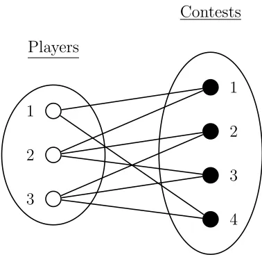
Figure 1: The contest network as a bipartite graph.

Figure 1 illustrates the bipartite structure of the network. In this figure, player 1 competes in two contests (dp₁ = 2); players 2 and 3 each compete in three contests (dp₂ =

dp₃ = 3); and 2 players compete in each contest (dc

m = 2 for each contest m = 1,2,3,4). The bipartite network structure is summarized by the N ×M biadjacency matrix:

g=



    

g11 g12 · · · g1M

g21 g22 · · · g2M ... ... ... ...

gN1 gN2 · · · gN M



    

.

For the network structure in Figure 1:

g =



 

1 0 0 1 1 1 1 0 0 1 1 1



 .

Denote by x = (x1, . . . , xN) the vector of all players’ efforts. For a given network structure, g, and vector of efforts, x, let pim(x,g) denote the probability that player i wins contest m. The function, pim(·) is the contest-success function (CSF). Note that

pim(x,g) = 0 if gim = 0. Moreover, we assume that pim depends only on the efforts allocated to contest m, and does not depend on the outcomes of other contests.

The expected payoff to player i is the sum of the expected payoffs across contests in

which she competes; it is given by,

πi(x,g) =

X

m∈M

pim(x,g)V −xi. (1)

Player i takes the strategies of the other N −1 players and the network structure as given, and chooses xi to maximize πi. Before proceeding to the analysis, there are a few network structures worth mentioning.

Biregular Networks

A bipartite network, g, isbiregular if each pair of nodes in the disjoint subsets ofg have the same degree. In our context, this means each player competes in the same number of contests, and each contest has the same number of participants. We provide the following definition:

Definition 1. Biregular Network

The bipartite network, g, is biregular if for all contests m, n ∈ M, and all players i, j ∈ N:

1. Contest Symmetry: dc

m =dcn =dc

2. Player Symmetry: dpi =d p j =dp

In terms of the biadjacency matrix, for a biregular network the sum across each row is equal to dp_{, and the sum down each column is equal to d}c_{. Studying Figure 1, it is} clear that this is not a biregular network; while each contest has 2 participants (so Part 1 of Definition 1 is satisfied, withdc_{= 2), player 1 competes in 2 contests, while players} 2 and 3 each compete in 3 contests; thus, Part 2 of Definition 1 is not satisfied.

A biregular network with N players, M prizes, contest degree, dc_{, and player degree,}

dp_{, can be summarized by [N, d}p_{;M, d}c_{]. From the degree definitions (and our assumption} that dc

m ≥2) it follows,

2≤dc_{≤N (2)}

and

1≤dp ≤M. (3)

Note that the following link property must hold for biregular networks:

The left-hand side of (4) gives the number of links from players to prizes. The right-hand side of (4) gives the number of links from prizes to players. Clearly, these numbers must be the same. Two special cases of biregular networks are complete networks, and circle networks.12 _{We provide the following definitions:}

Definition 2. Complete Network

A biregular network is complete if dc _=N.

Definition 2 says that the biregular network is complete if each contest has N partic-ipants. Note that the link property (4) implies that in a complete network, each player competes for all M prizes; i.e., dp _{= M. This means that there is always a unique} com-plete network for any givenN and M. We next define a circle network. Before doing so, we will need to introduce some additional terminology: A walk is a sequence of nodes,

`1, . . . , `k, where `i ∈ N ∪ M, and for each i from 1 to k−1, `i is linked to `i+1.13 The

length of the walk is equal to the number of links; i.e., k−1. A path is a walk`1, . . . , `k such that each pair of nodes is distinct, `i 6=`j, with the possible exception that`1 =`k. A cycle `1, . . . , `k is a path such that `1 =`k.

Definition 3. Circle Network

A biregular network is a circle if dc _=dp _{= 2, and there is a cycle of length 2N.} In a circle network, each player competes in two contests, and each contest has two participants (i.e., dp _{= d}c _{= 2), but no two contests have the same set of participants.} Note that the link property, (4), then impliesN =M. Example 1 describes all biregular networks for the case of N = 3; Figure 2 illustrates the corresponding networks.

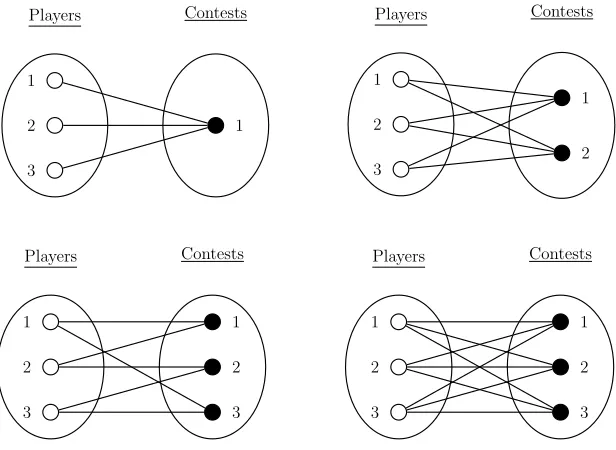
Example 1. Suppose that there are N = 3 players.

• If M = 1, then there exists a unique biregular network. In this network, dc_{= 3 and}

dp _{= 1.}

• If M = 2, then there exists a unique biregular network. In this network, dc_{= 3 and}

dp _{= 2.}

• If M = 3, then there exist two biregular networks: 1. A circle network where dc _=dp _{= 2.}

2. A complete network where dc_=dp _{= 3.}

12_{Circle networks are also known as cycle graphs or ring networks.} 13_{For instance, if`}

1 ∈ N, andk is odd then it must be that`k ∈ N. If there is a walk from `1 to `k

1 2 3 1 2 3 4 Players Contests 1 2 3 1 Players Contests 1 2 3 1 2 Players Contests 1 1 2 3 1 2 3 Players Contests 1 2 3 1 2 3 Players Contests P1 P2

(a) 2-Player Contest

P1 P2

P3

P4

(b) 4-Player Circle

P2 P1 P6 P5 P4 P3

(c) Complete Network

Figure 3: 3 Examples of symmetric contest networks. Players are represented as hollow nodes and prizes are represented as solid nodes. Each player competes for the prize(s) to which she is connected.

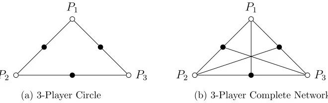
P2

P1

P3

(a) 3-Player Circle

P2

P1

P3

(b) 3-Player Complete Network

Figure 4

2

Figure 2: Illustration of the four networks described in Example 1. For all four networks,N = 3. Top left: M = 1,dc_{= 3,d}p_{= 1; Top right: M =d}p_{= 2,d}c_{= 3; Bottom left: A circle network withM = 3,}

dc_=dp_{= 2; Bottom right: A complete network with M =d}c _=dp_{= 3.}

Star Networks

In a star network there areM contests and N =M + 1 players: M “periphery players” and 1 “central player”. Each periphery player competes in a single contest, while the central player competes in all M contests. The winner of each contest receives a prize,

V >0.

Definition 4. Star Network

Let g be a network such that|M| =M ≥2and |N |=M+ 1. The network is a star if (1) each contest k ∈ M has degree 2, i.e., dc

k = 2; (2) there is a “central player” i

∗ _{∈ N}

that has degreeM, i.e., dp_i∗ =M; and (3) each “periphery player” j ∈ N \ {i∗}has degree

1, i.e., dp_j = 1.

Figure 3 illustrates a star network whereM = 5. As a convention, we will label the central player of a star network as playerM + 1; so, the set of periphery players is {1, . . . , M}.

Hybrid Networks

P3

P2

P1

P5

P4

Figure 5: Star Network with N = 5 periphery players/prizes

P2

P1

P3

P4

Figure 6

P2

P1

P6

P5

P4

P3

P7

Figure 7: Hybrid Network

Figure 3: A star network withM = 5. Players are represented by hollow nodes; contests are represented by solid nodes.

structure as aσ-hybrid network.14 _{We provide the following definition:}

Definition 5. σ-Hybrid Network

Let g be any biregular network with N players and M prizes. A σ-hybrid network is the network, g0, formed by adding an additional player to g, who competes for σ ≤ M prizes. We call g the underlying network of g0. We refer to the players in g, {1, . . . , N}, as the underlying players of g0, and we call the additional player, N+ 1, the hybrid player of g0.

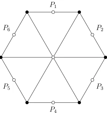
Figure 4 illustrates a 6-hybrid network where the underlying network is a 6-player circle.

3

A Unified Framework

In this section we show that a number of important results from the contest literature can be obtained as special cases of our network framework. Section 3.1 sets up the model under the Tullock CSF, and provides an explicit characterization of equilibrium for certain network structures of interest. Section 3.2 provides an analogous analysis for the APA CSF. Section 3.3 unifies our results with the existing literature on contests. All proofs are contained in the Appendix.

P3

P2

P1

P5

P4

Figure 5: Star Network with N = 5 periphery players/prizes

P2

P1

P3

P4

Figure 6

P2

P1

P6

P5

P4

P3

Figure 7: Hybrid Network

3

Figure 4: A 6-hybrid network. The underlying network is a 6-player circle. Players are represented by hollow nodes; contests are represented by solid nodes.

3.1

Tullock CSF

We now extend the classical Tullock contest to our network contest environment. Fix a network structure,g, and letx−i ∈RN+−1 denote the vector of efforts chosen by all players

other than some player i. If P

j∈N gjmxj >0 for some prize m, then the probability that player i wins prize m is given by the following contest success function:

pim(xi,x−i,g) =

gimxri

P

j∈Ngjmxrj

.

The parameter r >0 measures the sensitivity of the probability of success to players’ effort choices. A higher value of r corresponds to a contest success function that is more sensitive to players’ efforts. If P

j∈N gjmxj = 0 for some contestm, then we assume that each player linked to m is equally likely to win: pim(·) = g_dimc

m. Using equation (1), the

expected payoff to playeri may then be written:

πi(xi,x−i,g) =

X

m∈M

gimxri

P

j∈Ngjmxrj

V −xi.

an interior solution, the first-order condition for player i is,

∂πi(xi,x−i,g)

∂xi = X m∈M         

rxr−1

i

P

j∈Ngjmxrj

−rx2r−1

i

P

j∈Ngjmxrj

2 gimV         

−1 = 0. (5)

In a pure-strategy equilibrium in which each player is active (i.e. chooses a strictly positive effort level), equation (5) is satisfied for each playeri.

Characterizing Equilibrium

Equation (5) characterizes equilibrium for general network structures (when all players are active). We will now provide closed-form expressions for equilibrium efforts for cer-tain network structures of interest. It will be seen in Section 3.3 that these networks have interesting connections with the existing contest literature. We will focus on “sym-metric” equilibria. By symmetric in this context, we mean that symmetric players follow symmetric strategies.

To begin, suppose that the network is biregular, summarized by [N, dp_{;M, d}c_{], where}

dc_{≥2. In a biregular network, all players are symmetric; so, in a symmetric equilibrium,}

x∗

i = x

∗

j = x

∗ _{for each i, j ∈ N. Imposing symmetry, for each i ∈ N, equation (5)}

simplifies to, X m∈M         

rx∗r−1

P

j∈Ngjmx∗r

−rx∗2r−1

P

j∈N gjmx∗r

2 gimV

        

−1 = 0. (6)

Applying the properties of biregular networks given in Definition 1 to equation (6), our first result characterizes the unique symmetric equilibrium of biregular networks.

Lemma 1. Suppose that the network is biregular and summarized by[N, dp_{;M, d}c_{]. Under}

the Tullock CSF there exists a symmetric pure-strategy equilibrium if and only ifr ≤ dc

dc₋₁.

The symmetric equilibrium is unique, and equilibrium individual effort, x∗_{, is given by,}

x∗ = r(d c₋₁₎ (dc₎2 d

p

Total equilibrium effort is,

X∗ =N x∗ = r(d c₋₁₎

dc M V.

Next, consider a star with M contests. Suppose that each of the M symmetric pe-riphery players follow symmetric strategies. Let x∗ _{denote the equilibrium effort of each}

periphery player, and let x∗

M+1 denote the equilibrium effort of the central player. For

each periphery player, (5) reduces to,

rx∗r_x∗r−1

M+1

(x∗r_+x∗r M+1)2

V = 1. (7)

While for the central player, (5) becomes,

M

X

i=1

rx∗r_x∗r−1

M+1

(x∗r_+x∗r M+1)2

V −1 = 0. (8)

Our next result characterizes the unique symmetric equilibrium when the network is a star.

Lemma 2. Suppose the network is a star with M contests. Under the Tullock CSF there exists a symmetric pure-strategy equilibrium if and only ifrMr _≤Mr_{+ 1. The symmetric}

equilibrium is unique, and effort for each periphery player is, x∗ = rM

r

(Mr_{+ 1)}2V.

The effort of the central player is x∗

M+1 =M x∗. Total equilibrium effort is,

X∗ =M x∗+x∗M+1 =

2rMr+1

(Mr_{+ 1)}2V. (9)

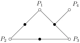
Finally, consider a σ-hybrid network. In contrast to biregular and star networks, for hybrid networks, there may not exist a symmetric equilibrium in which every player is active (i.e. exerts strictly positive effort). In particular, unlessσis large enough, there will always exist a symmetric equilibrium in which the hybrid player is inactive (i.e., exerts zero effort). We illustrate this finding first via an example, and then we provide a general result.

symmetric equilibrium, x∗

1 = x∗3. Under the Tullock CSF with r = 1, it may be verified

that there is only one symmetric equilibrium, and in this equilibrium, x∗

1 =x∗2 =x∗3 = V2;

and x∗

4 = 0.

P3

P2

P1

P5

P4

Figure 5: Star Network with N = 5 periphery players/prizes

P2

P1

P3

P4

Figure 6

P2

P1

P6

P5

P4

P3

P7

Figure 7: Hybrid Network

3

Figure 5: A 1-hybrid network in which the underlying biregular network is a 3-player circle. Players are represented by hollow nodes; contests are represented by solid nodes.

Our next result generalizes the finding of Example 2, and shows that, in a 1-hybrid, there always exists an equilibrium in which the hybrid player is inactive, so long as each of the other players compete in at least 2 contests.

Lemma 3. Consider a 1-hybrid network, g0, with the underlying network, g, where g is summarized by [N, dp_{;M, d}c_{] with d}p _{≥2. Under the Tullock CSF (r = 1) there exists an}

equilibrium in which the hybrid player is inactive, and the effort of each underlying player is given by,

x∗ = (d c₋₁₎ (dc₎2 d

p_V.

Example 2 and Lemma 3 suggest that when an additional player is added to a sym-metric network, that player must compete in several contests in order to have an incentive to actively participate. We will next consider the extreme case of M-hybrid networks, in which the hybrid player competes for all M prizes in the underlying network. Figure 4 illustrates anM-hybrid network in which the underlying network is a 6-player circle.

Lemma 4. Suppose the network is an M-hybrid with an underlying biregular network summarized by [N, dp_{;M, d}c_{]. Under the Tullock CSF with r = 1 there exists a unique}

symmetric equilibrium. In this equilibrium, effort for each underlying player is, x∗ = N

(N + 1)2d

p

V.

The effort of the hybrid player is,

x∗N+1 = (N + 1−d

Total equilibrium efforts is,

X∗ =N x∗+x∗_N+1 = (2N + 1−d c_)N (N + 1)2 d

p_V.

3.2

APA CSF

In this section we extend the all-pay auction to our network framework. Under the all-pay auction CSF, playeriwins contestm with certainty if her effort choice is greater than the effort exerted by the other participants of contestm. In the event that 2 or more players choose the same highest effort, these players are equally likely to win. Formally:

pim(xi,x−i,g) =

  

 

gim, if xi >maxj6=i{gjmxj}, 0, if xi <maxj=6 i{gjmxj},

gim

n , if ities with n−1 others for the highest bid.

It is well-known that the APA with complete information does not possess a pure-strategy equilibrium. Denote byFj the CDF of player j’s mixed strategy, and let F−i = (F1, . . . , Fi−1, Fi+1, . . . , FN) denote the collection of (independent) distribution functions of all players other than playeri. If player i chooses effort xi then,

pim(xi,F−i,g) = gim

Y

j6=i

Fj(xi)gjm.

The expected payoff for player i is,

πi(xi,F−i,g) =

X

m∈M

gim

Y

j6=i

Fj(xi)gjm

!

V −xi.

Let Si ⊆R+ denote the support of player i’s mixed strategy. In equilibrium, for each

player i, and eachx, x0 _∈

R+,

x, x0 ∈Si =⇒ πi(x,F−i,g) = πi(x0,F−i,g)

and

Characterizing Equilibrium

We now provide an explicit characterization of equilibrium distribution functions for the network structures of interest. Before proceeding, note that in a single-prize contest under the APA CSF there typically exist many equilibria, including a continuum of asymmetric equilibria when all players have a common prize value (see Baye et al., 1996, henceforth, BKD). However, there typically exists a unique symmetric equilibrium. In our analysis, we will focus on “symmetric” equilibria. As in Section 3.1, when we say “symmetric” in this context, we mean that symmetric players follow symmetric strategies. We now characterize equilibrium for biregular networks under the APA CSF.

Lemma 5. Suppose the network is biregular. Under the APA CSF there is a unique sym-metric equilibrium in which each player randomizes continuously on the interval [0, dp_V]

according to the CDF,

F∗(x) = x

dp_V

_dc1₋₁

. (10)

The equilibrium expected payoff to each player is zero. The expected total equilibrium effort is

X∗ = N d p

dc V =M V.

Our next result characterizes the unique symmetric equilibrium for a star network.

Lemma 6. Suppose the network is a star with M contests. Under the APA CSF there exists a unique symmetric equilibrium in which the central player randomizes uniformly on

[0, V], while each periphery player places an atom at 0 of size α= M−1

M , and randomizes

continuously on (0, V] according to the CDF, F∗(x) = M −1

M + x M V.

The expected payoff of the central player is(M−1)V. The expected payoff of each periphery player is zero, and the expected total equilibrium effort is,

X∗ =V.

Lemma 7. Consider a 1-hybrid network, g0, with an underlying network, g, where g is summarized by[N, dp_{;M, d}c_{] withd}p _{≥2. Under the APA CSF there exists an equilibrium}

in which the hybrid player is inactive, and each underlying player randomizes continuously on [0, dp_{V] according to the CDF,}

F∗(x) = x

dp_V

_dc1−1

.

Finally, we characterize equilibrium under the APA CSF when the hybrid player com-petes for allM of the contests.

Lemma 8. Suppose the network is an M-hybrid with an underlying network summarized by [N, dp_{;M, d}c_{]. Under the APA CSF there exists a unique symmetric equilibrium in}

which each underlying player places an atom of sizeα = M−dp

M

_dc1

at zero, and randomizes continuously on (0, dp_{V] according to the CDF,}

F∗(x) =

M−dp

M + x M V

_dc1

.

The hybrid player randomizes continuously on [0, dp_{V] according to the CDF,}

G∗(x) = x

dp_{V F(x)}dc₋₁.

The expected payoff of the hybrid player is (M − dp_{)V. The expected payoff of each}

underlying player is zero, and the expected total effort is equal to X∗ =dpV.

3.3

Unification

In this section, we unify the results of Sections 3.1-3.2 with the existing literature on contests.

Symmetric Contests

We begin by showing a connection between behavior in single-prize symmetric contests and behavior in our model when the network structure is biregular.

and expected payoffs in adc_{-player contest in which players compete for a single prize with}

common value dp_{V. Total equilibrium effort is equivalent to total equilibrium effort in a}

dc_{-player contest in which players compete for a single prize with common value M V.} Theorem 1 establishes a connection between behavior in the contest played on the network, and behavior in symmetric single-prize contests, absent network effects. Consider a biregular network summarized by [N, dp_{;M, d}c_{]; in this network each of the N players} competes for dp _{prizes, and each contest has d}c _{participants. Each player thus competes} for a total value ofdp_{V, while the total value of all prizes is M V. Theorem 1 establishes} that each player behaves “as if” competing in adc_{-player contest in which each player has} common valuedp_{V, while total equilibrium effort is “as if” d}c _{players each compete for a} prize of common valueM V.

To further illustrate this result, consider, for concreteness, the three-player circle illus-trated in the bottom-left panel of Figure 2. In this network, each player competes in two contests, and each contest has two participants. In equilibrium, each player behaves as if competing for a single prize of size 2V against one other player. To see this connection, first consider a two-player contest with players A and B, who each compete for a single prize of size 2V, and suppose the CSF is the Tullock. Let x∗ _{denote the (unique)}

sym-metric equilibrium effort level in this game. If player A chooses effort, xA, and B plays according to equilibrium,xB =x∗, then the payoff to player A is:

πA(xA, xB =x∗) =

xr A

xr A+xrB

2V −xA=

xr A

xr A+x∗r

V + x r A

xr A+x∗r

V −xA. (11)

Now, in the 3-player circle network, if Player 1 (say) chooses effortx1, while players 2 and

3 each choose effort,x∗_{, then the payoff to Player 1 is the sum of the payoffs she receives}

from the contest with Player 2 and with Player 3:

π1(x1, x2 =x∗, x3 =x∗,g) =

xr

1

xr

1+xr2

V + x r

1

xr

1+xr3

V −x1

= x

r

1

xr

1+x∗r

V + x r

1

xr

1+x∗r

V −x1. (12)

Clearly, the payoff to player A in equation (11) is the same as the payoff to player 1 given in equation (12). Since, by definition, x∗ _{maximizes the payoff to A, it must also}

response is also to choose x∗_.15 _{An analogous symmetry holds under the APA CSF.}

It is also worth mentioning that the standard comparative statics results from the contest literature hold in our setting when the network is biregular. Specifically, for either the APA or Tullock CSF, expected individual and total equilibrium effort are increasing in the prize valueV. In addition, under the Tullock CSF, individual and total equilibrium efforts are increasing in the noise parameter, r, and for any r such that a pure strategy equilibrium exists under the Tullock, expected total effort is higher under the APA than under the Tullock CSF.

Asymmetric Contests

Our next result establishes a connection between equilibrium behavior in the star network with equilibrium behavior in 2-player asymmetric contests.

Theorem 2. Suppose the network is a star and the CSF is either the Tullock or APA. Individual equilibrium behavior and expected payoffs are equivalent to the behavior and expected payoffs in a 2-player asymmetric contest in which the “weak” player has value,V, while the “strong” player has value, M V. Each periphery player behaves as-if competing as the weak player, while the central player behaves as-if competing as the strong player in the 2-player contest.

Theorem 2 establishes a close connection between a contest played on a star network and 2-player asymmetric contests. To see this connection more explicitly, consider a star network with M contests. Note that the payoff to a periphery player, i, only depends directly on her own effort and the effort of the central player. So, letπi(x, xM+1) denote

the payoff to player i when she chooses effort x, and the central player, M + 1, chooses effort xM+1. Under the Tullock CSF,

πi(x, xM+1) =

xr

xr_+xr M+1

V −x. (13)

The expected payoff to the central player depends on her own effort as well as the efforts of each periphery player. Suppose the periphery players choose efforts according to x = (x1, . . . , xM). Then, the central player’s expected payoff, πM+1(xM+1,x), is given by,

πM+1(xM+1,x) =

M

X

i=1

xr M+1

xr

i +xrM+1

V −xM+1.

15_{Given the symmetric nature of the network, our choice to examine the payoff of Player 1 was arbitrary;}

If the periphery players follow symmetric strategies, so that x = (x, . . . , x), then the expected payoff to the central player reduces to,

πM+1(xM+1,x) =

xr M+1

xr

M+1+xr

M V −xM+1. (14)

Studying expressions (13) and (14) it is clear that, when the periphery players adopt symmetric strategies, the expected payoff of the central player is equivalent to what his payoff would be in a two-player Tullock contest in which he has value M V and his opponent chooses effort, x. Moreover, the expected payoff to each periphery player is equivalent to what her payoff would be in a two-player contest in which she has value

V. A similar symmetry holds under the APA CSF. Note, however, that total equilibrium effort on the star is greater than it would be in a 2-player asymmetric contest. This is clearly the case since, on the star network, there are M ≥ 1 periphery players, each of whom behaves as they would in the 2-player contest.

As shown in Section 3.1, for biregular networks under the Tullock CSF total equilib-rium effort is linear and increasing in r. This result is consistent with findings in the contest literature when players have the same prize values. When the prize values are different, Nti (1999, 2004) shows that this relationship is less clear, and is generally not monotonic. We obtain a similar finding in our setting when the network is a star.

In what follows, we restrict attention to values of r that permit the existence of a symmetric pure-strategy equilibrium. LetrM denote the unique solution to the equation

(rM −1)MrM = 1. (15)

rM is the highest value of rthat supports a symmetric pure-strategy equilibrium on a star with M periphery players (see Lemma 2). Clearly, for any M, rM >1. Moreover, it is straightforward to show that rM is strictly decreasing in M, andrM ∈(1,2].16

Let X∗

M(r) denote total equilibrium effort when there are M periphery players, and the Tullock CSF parameter is r. Let r∗_{(M) denote the value of r that maximizes total}

equilibrium effort:

r∗_{(M) = arg max}

r∈[0,rM]

{X∗

M(r)}.

Our next proposition reveals that total equilibrium effort is in fact a single-peaked function

16_{It is well-known that forr∈(2,∞) there does not exist a pure-strategy equilibrium under the Tullock}

ofr. Moreover, we show that for any fixedr∈(0, rM), total equilibrium effort is increasing inM. That is, as the number of periphery players (and prizes) increases, total equilibrium effort increases.

Proposition 1. Suppose the network is a star with M ≥ 2 contests, and the CSF is the Tullock. Equilibrium total effort, X∗

M(·), is a single-peaked function, and r

∗_{(·) is a}

single-valued function. If M ≥4, then r∗_{(M)∈(0, r}

M) and r∗(M) is characterized by,

r∗(M) ln(M) = M

r∗(M)_{+ 1}

Mr∗_(M)

−1.

Further, r∗_{(·) is strictly decreasing and lim}

M→∞r∗(M) = 0. Finally, for any M ≥2

and r such that r ∈(0, rM+1), it holds that XM∗ +1(r)> XM∗ (r).

We first convey the intuition behind the relationship between equilibrium total effort and the parameter r. Nti (1999) shows that the fraction of each player’s rent that is dissipated in equilibrium in the asymmetric two-player Tullock contest is non-monotonic inr. Drawing on the equivalence between individual equilibrium behavior in Nti’s setting and our setting, consider the setting studied by Nti. For fixed prize values, whenris close to zero, the outcome of the contest is largely determined by luck. As a result, players do not have strong incentives to exert effort. As r increases, the outcome of the contest depends less on chance, and more on players’ efforts. This provides stronger incentives for both players to exert effort. However, if the contest is asymmetric enough, as r increases further, the stronger player – who always exerts more effort than the weaker player – becomes ever more likely to win the contest. This discourages the weaker player from exerting effort, which may also mean that the strong player need not exert much effort in equilibrium. Combining these two effects gives rise to a non-monotonic relationship between r and total effort.

In our setting, a higher value of M corresponds to a greater degree of asymmetry in the contest; for M large enough, the value of r that maximizes total effort will be in the interior of the feasible set; i.e., r∗(M) ∈ (0, rM). As M gets larger, the degree of asymmetry grows, and the discouragement effect described above is exacerbated. Lower values of r introduce a greater amount of chance into each contest, which dampens this effect by reducing the advantage of the stronger player. As a result, r∗_{(·) is decreasing.}

Finally, asM gets large, the only way to prevent complete discouragement of the periphery players is by choosingr closer to zero, and so r∗_{(M) approaches zero asM gets large.}

First, as already discussed, increasingM increases the degree of asymmetry in the contest, which is akin to increasing the prize value of the strong player in Nti’s (1999) setting. Nti shows that, ceteris paribus, an increase in the strong player’s prize value increases his effort, and reduces the effort of the weaker player. The net effect on total effort is ambiguous. But there’s a second channel in our setting that is absent in Nti’s setting; an increase in M also increases the number of periphery players. Although the individual effort of each periphery player decreases, it can be shown that the combined effort of these M periphery players is increasing in M. The net effect is that an increase in M

unambiguously increases total equilibrium effort under the Tullock CSF.

We next compare the total equilibrium effort on the star under the Tullock and APA CSFs. Recall that on biregular networks, equilibrium total effort is always greater under the APA CSF than under the Tullock CSF. Our next result shows that for star networks, the opposite conclusion may hold.

Proposition 2. Suppose the network is a star with M contests. Fix r= 1, and suppose thatM ≥3. Then equilibrium total effort is higher under the Tullock CSF than under the APA CSF.

The intuition for Proposition 2 closely relates to that of Proposition 1. As shown in Proposition 1, under the Tullock CSF total equilibrium effort may be decreasing in r

when M is sufficiently large. But the APA CSF is just the limiting case of the Tullock CSF as r → ∞. As a result, when M is sufficiently large (in this case, M ≥ 3), so that there is a sufficient degree of asymmetry in the network, the less cutthroat competition induced under the Tullock generates greater total effort in equilibrium.

The Exclusion Principle

the remaining players to offset the drop in effort caused by the removal of he high-value player.

We next explore this idea in our network setting. To do so, we compare the expected total equilibrium effort on an M-hybrid network, with the total effort of the underlying network. We obtain an exclusion result akin to that of Baye et al under the APA CSF. In contrast to Fang’s result, we show that a similar exclusion result also holds under the Tullock CSF in our setting. Before proceeding, let x(g) denote individual expected equilibrium effort when the network isg, and letX(g) denote equilibrium expected total effort.

Theorem 3. Let g0 be an M-hybrid network with an underlying network, g, summarized by [N, dp_{;M, d}c_{]. Under the APA CSF, X(g)> X(g}0_{) if and only if N > d}c_{. Under the}

Tullock CSF, X(g)> X(g0) if and only if N > (d

c₎2_{+ 1}

dc₋₁ . (16)

Theorem 3 establishes that if the network structure is an M-hybrid, then a contest designer may be able to increase total equilibrium effort by excluding the hybrid player. Under the APA CSF, this exclusion result holds so long as there issome degree of asym-metry between the hybrid player and the underlying players in the network, which mirrors the results of Baye et al. (1993).

Our exclusion result under the Tullock CSF contrasts existing results from the contest literature (see, e.g., Fang, 2002; Matros, 2006). The condition given in (16) can be interpreted as requiring a sufficient degree of asymmetry in the hybrid network. To see this, note that (16) requires thatN is sufficiently large, relative todc_{. By the link property} of biregular networks, N dp _{=M d}c_{, whenN is large, relative tod}c_{it must mean thatd}p _is small, relative to M. That is, the hybrid player, who competes in M contests, competes for sufficiently more prizes than each player in the underlying network (each of these players compete fordp _prizes).

The impact on aggregate behavior of adding a or removing a player from a network, not only depends on that player’s direct contribution, but also depends on indirect effects that stem from the player’s influence on the structure of interactions (see, e.g. Ballester et al., 2006). Previous results on the Exclusion Principle in the contest literature mainly focus on one particular pattern of interactions (one in which all players compete for a single prize); the addition/removal of one player does not affect this structure.17 _When

indirect network effects are taken into account, our Theorem 3 suggests that the Exclusion Principle is a more robust phenomenon than previously thought. The following example illustrates our finding.

Example 3. Suppose g0 is an M-hybrid with an underlying network, g, where g is sum-marized by [N, dp_{;M, d}c_{] = [6,2; 4,3]. Consider the Tullock CSF with noise parameter}

r= 1, and assume V = 1. Under the APA CSF: X(g) =M V = 4

and,

X(g0) =dp_{V = 2.}

Under the Tullock CSF:

X(g) = (d c₋₁₎

dc M V = 8

3 ≈2.667

and,

X(g0) = (2N + 1−d c_)N (N + 1)2 d

p_{V =} 120

49 ≈2.449.

Summarizing

In this section, we have shown that a number of results from the contest literature can be obtained by varying the structure of the network in our framework. Table 1 summarizes these linkages.

Table 1: A Unified Framework

Contest Results and Corresponding Network Structures

Result Related Literature Network Structure

Behavior in

Symmetric Contests

Tullock (1980), Hillman and Riley (1989),

BKD Biregular Networks

Behavior in

Asymmetric Contests

Hillman and Riley (1989), BKD, Nti (1999, 2004), Stein (2002), Matros (2006)

Star Networks

Exclusion Principle Baye et al. (1993), Fang (2002),

Matros (2006), Menicucci (2006) M-Hybrid Networks

4

Network Structures

In this section, we explore how the underlying network structure affects equilibrium be-havior. Consider two biregular networks, g1 and g2, each with N players. Summarize

networkgk by [N, dp_k, Mk, dck]. Our interest is in assessing how equilibrium behavior varies with the network parameters, N, dp_{, M, or d}c_{. Let V}

k denote the prize value associated

with each contest when the network structure is gk. We wish to distinguish the impact of a change in the network structure from, say, an increase in the total value for which players compete; so, we assume that the total value of all prizes in each network is the same: M1V1 = M2V2. Note that since the link property, N dp =M dc, must hold for the

network to be biregular, one can not assess a ceteris paribus change in one of the network parameters, and simultaneously preserve biregularity. Nevertheless, our next result cap-tures some sense in which equilibrium behavior is affected by a change to the structure of the network.

Theorem 4. Let g1 and g2 be two biregular networks with N players, such that the total

value of all prizes in each network is the same: M1V1 = M2V2. Then under the Tullock

CSF, the following four statements are equivalent: (i) dp₁V1 > dp2V2

(ii) dc

1 > dc2

(iv) x(g1)> x(g2)

Under the APA CSF, X(g1) =X(g2) and x(g1) =x(g2).

Theorem 4 describes how total and individual equilibrium efforts are affected when the structure of the network changes, but where the number of players, and the total value of all prizes in each network is held constant.

To illustrate the result of Theorem 4, consider the two network structures in Figure 6. In each network, there are three players and three prizes. So, if each prize in both networks is worth V, then the total prize value in each network is 3V. Note that in the circle network of Figure 6(a), dp _{= d}c _{= 2; while in the complete network in Figure} 6(b) dp _=dc_{= 3. Theorem 4 implies that under the Tullock CSF, the complete network} generates greater individual effort than the circle network. Consider changing the network structure from the circle network to the complete network. Equilibrium efforts are affected via two channels. First, in the complete network, each player competes for a greater total value (3V as compared to 2V); this effect encourages greater effort from each player. Second, in the complete network, each player faces more competition in each contest. Examining the expression for individual effort in Lemma 1, it is clear that an increase in the number competitors (dc_{) decreases individual efforts. As it happens, the first} effect always dominates the second effect under the Tullock; hence, the complete network generates greater total effort than the circle. Under the APA CSF, these two effects exactly offset one another, leading to the same total and individual expected efforts for either network structure.

Theorem 4 is also useful for providing insights into the optimal design of networks. Suppose there are a fixed number of players,N, and a contest designer with a prize budget of B. The designer chooses a biregular network, with the goal to maximize the sum of

1

2

3

1

2

3

Players _Prizes

1

2

3

1

2

3

Players _Prizes

P1

P2

(a) 2-Player Contest

P1 P2

P3

P4

(b) 4-Player Circle

P2

P1

P6

P5

P4

P3

(c) Complete Network

Figure 3: 3 Examples of symmetric contest networks. Players are represented as hollow nodes and prizes are represented as solid nodes. Each player competes for the prize(s) to which she is connected.

P2

P1

P3

(a) 3-Player Circle

P2

P1

P3

(b) 3-Player Complete Network

Figure 4

equilibrium efforts. In other words, the designer takes N and B as given, and choosesdp_,

M, and dc _{to maximize total equilibrium effort, subject to the constraints N d}p _{= M d}c andM V =B.18 _{As a straightforward consequence of Theorem 4, under the Tullock CSF,}

the designer would be indifferent between any complete network structure. This must be true since, in general dc _{≤ N, and for a complete network structure, d}c _{= N. Part (ii)} of Theorem 4 immediately implies that this network structure would indeed maximize equilibrium efforts, subject to the aforementioned constraints. The following numerical example illustrates.

Example 4. Let gbe a biregular network where N = 3. Suppose that B = 12 and r= 1. Denote by X∗ _{total equilibrium effort under the Tullock CSF.}

• If M = 1, there is a unique biregular network, and this network is complete: dp _{= 1}

and dc_{= 3. Total equilibrium effort is}

X∗ = r(d c₋₁₎

dc M V = 2

3B = 8.

• If M = 2, there is a unique biregular network, and this network is complete: dp _{= 2}

and dc_{= 3. Total equilibrium effort is}

X∗ = r(d c₋₁₎

dc M V = 2

3B = 8.

• If M = 3, then there are two biregular networks:

1. A complete network: dp _=dc_{= 3, which yields total effort of}

X∗ = r(d c₋₁₎

dc M V = 2

3B = 8.

2. A circle network: dp _=dc_{= 2, which yields total effort of}

X∗ ₌ r(dc−1)

dc M V = 1

2B = 6.

Next, suppose the number of prizes is fixed at M, and consider adding a player to a biregular network, g. The resulting network structure, g0 is thus a σ-hybrid. We

18_{There is no reason to think that a contest designer should be restricted to only choosing a symmetric}

have already shown in Lemmas 3 and 7 that, unless σ is sufficiently large, there will always exist an equilibrium in which the additional player is inactive, and there is no impact on the behavior of the players in g. Moreover, we showed in Theorem 3 that if this additional player competes in every contest, and the resulting network structure is asymmetric enough, then the equilibrium effort of each player in g will decrease, and total effort in g0 is lower than in g. Finally, consider adding an additional player to a biregular network in such a way that the biregularity of the network is preserved. Since the link property, N dp _{=M d}c_{, must hold, it only make sense to answer this question for} complete networks. In a complete network, N = dc_{. By Lemma 1 it is clear that under} the Tullock CSF, individual equilibrium effort decreases, while total equilibrium effort increases, following the entry of an additional player. Under the APA CSF, Lemma 5 implies that total expected equilibrium effort is unchanged, and hence individual expected efforts must fall.

5

Conclusion

In this paper we have proposed a framework for studying contests on networks. We characterized equilibrium in terms of the underlying network structure, and studied how this structure affects equilibrium behavior. Furthermore, we have shown that a number of results from the contest literature may be obtained in our framework by varying the structure of the network. In addition, we have provided a new exclusion result, akin to Baye et al.’s (1993) Exclusion Principle, but which is relevant under the Tullock CSF. This result contrasts the existing literature, and highlights the relevance of network effects in our model.

6

Appendix

Proof of Lemma 1

Let x∗ _{be as given in the lemma. We will show that x}∗ _{is a best response to x}∗ −i ≡ (x∗, ..., x∗). Let Γ(xi,x−i) ≡ ∂πi(x_∂xi,x−i,g)

i . First, we show that Γ(x ∗

,x∗−i) = 0 and, for

r≤ dc

dc₋₁, the second order condition is satisfied. Finally, we will show thatπi(x∗,x∗−i)>0. Since the network is biregular, if player i competes in contest m (so that gim > 0), then P

j6=igjm =d

c_{−1. If player i does not compete in contest m, theng}

for each contest, m, it holds:

gim

P

j6=igjm

P

j∈Ngjm

2 =

dc₋₁ (dc₎2 gim.

Then, using (6),

Γ(x∗,x∗_−i) = rV

x∗ X m∈M         

gimP_j6=igjm

P

j∈Ngjm

2          −1 = rV x∗ X m∈M

dc₋₁ (dc₎2 gim

−1

=

r(dc₋₁₎ (dc₎2 d

p

V

1

x∗ −1 = 0.

To show that x∗ _{is in fact a best-reply to x}∗

−i we now show that the second-order condition is satisfied, and πi(x∗,x−∗i,g)≥0. The second-order condition for player iis

∂Γi(xi,x∗−i)

∂xi

|xi=x∗ =

(r−1)dc_−2r

dc rV (x

∗

)2r−2 M

X

m=1

(dc₋₁₎

= (r−1)d c_−2r

dc (d

c_{−1)rM V (x}∗

)2r−2 <0 (17)

The SOC given in equation (17) is satisfied if and only if (r−1)dc_{−2r <0, which holds} if dc _{= 2. If d}c _{> 2 then (17) holds if and only if r <} dc

dc₋₂, which is satisfied under the

condition,r < dc

dc₋₁, given in the lemma. Next, we show thatπi(x∗,x∗−i,g)≥0. Note that

πi(x∗,x∗−i,g) = M

X

m=1

(

gimx∗r

PN

j=1gjmx∗r

V

)

−x∗ = d p_V (dc₎2

dc_−r(dc₋₁₎

.

The term in square brackets on the right-hand side (RHS) of the expression above is positive if and only if r≤ dc

dc₋₁, which establishes that x

∗ _{is a best-reply to x}∗ −i.

Now, we show that (x∗_{, ..., x}∗_{) is the unique symmetric equilibrium. Any symmetric}

equilibrium, (x0_{, . . . , x}0_{), must satisfy Γ(x}0_,x0

−i) = 0. However, it is straightforward to show that Γ(x, x, . . . , x) is strictly decreasing in x. Hence, there is a unique solution to Γ(x0_,x0

Proof of Lemma 2

Suppose the network is a star withN periphery players. The first-order condition for each periphery player i∈ {1, . . . , M} is given in equation (7), and the first-order condition for the central player, M + 1, is given in (8).

Equations (7) and (8) together imply:

xM+1 =

M

X

i=1

xi. (18)

Suppose that each periphery playeri adopts a symmetric strategy: xi =x. Then (18) implies thatxM+1 =M x. Using equation (7) it is easily verified that

x=x∗ = M r

(1 +Mr₎2rV.

Next, we confirm that the second-order conditions are satisfied. Note that for a star network, the payoff to each periphery player only depends directly on the effort of the central player. So, let πi(x, xM+1) denote the payoff to a periphery player, i, when she

chooses effort,x, and the central player choosesxM+1. It may be verified that the

second-order sufficient condition for periphery player i, ∂2πi(xi,x∗M+1) ∂x2

i |xi=x

∗ <0, is satisfied if and

only if rMr _{< M}r_{+ 1 +r, which is implied by the condition rM}r _{≤ M}r_{+ 1, given in} the lemma. It may be verified that the second-order condition for the central player is satisfied for anyM ≥1.

Finally, we show that πi(x∗, M x∗)≥0 if and only if rMr ≤Mr+ 1. Note that:

πi(x∗, M x∗) =

x∗r

x∗r_{+ (M x}∗₎rV −x

∗

= (1 + (1−r)M r₎

(1 +Mr₎2 V.

Thus, πi(x∗, M x∗)≥ 0 if and only if rMr ≤ Mr+ 1. Note that since each periphery player earns a non-negative payoff, the central player also earns a non-negative payoff.

Proof of Lemma 3

Let g0 be a 1-hybrid with an underlying network summarized by [N, dp_{;M, d}c_{]. Assume,} without loss of generality, that the hybrid player,N+1 competes in contest 1. To establish the lemma, it suffices to show that when each player i ∈ {1, . . . , N} chooses effort x∗_,

given in the lemma, then player N + 1 does not have a profitable deviation.

Suppose that each player i∈ {1, . . . , N} chooses effort x∗_{. Note that the total effort}

expended to each contest by these players is dc_x∗ ₌ dc₋₁

dc d

dc_{≥2 and d}p _{≥2 it holds thatd}c_x∗ ₌ dc₋₁

dc dpV ≥V. Suppose playerN+ 1 chooses effort

x∈_R+; the expected payoff to player N + 1 is:

πN+1(x,x∗,g0) =

x x+PN

j=1gj1xj

V −x

= x

x+dc_x∗V −x

≤x

V

x+V −1

≤0

The above inequality is strict if x >0. Hence, the only best response for player N + 1 is to choose x= 0.

Proof of Lemma 4

Consider some underlying player i ∈ {1, . . . , N}. Suppose that the underlying players other than i choose efforts according to, x−i = (x, . . . , x), where x >0, while the hybrid player chooses xN+1. If playeri chooses effort, xi, her expected payoff is:

πi(xi,x−i, xN+1) =

M

X

m=1

gimxi (dc_−1)x+x

i+xN+1

V −xi.

The first order condition is

∂πi(xi,x−i, xN+1)

∂xi

= M

X

m=1

(dc_−1)x+x N+1

((dc_−1)x+x

i+xN+1)2

gimV −1 = 0.

In a symmetric equilibrium, each underlying player chooses the same effort, xj = x∗ for

j ∈ {1, . . . , N}. The first-order condition becomes,

M

X

m=1

(dc_−1)x∗_+x

N+1

(dc_x∗_+x

N+1)2

gimV =

(g−1)x∗ _+x

N+1

(dc_x∗_+x

N+1)2

dp_{V = 1. (19)}

In a symmetric equilibrium, the payoff to the central player N + 1 is:

πN+1(xN+1,x∗) =

xN+1

dc_x∗_+x

N+1

The first order condition is

dc_x∗

(dc_x∗ _+x∗

N+1)2

M V = 1. (20)

From (19) and (20), we get

x∗_N+1 = d

c_{(M −d}p_{) +d}p

dp x

∗

= (N + 1−dc_)x∗

. (21)

From (4) and (21),

x∗

N+1 = (N + 1−g)x∗. (22)

Finally, (19) and (22) give

x∗ = N (N + 1)2d

p

V.

It is easy to verify that the second-order conditions are satisfied for all players. More-over, given efforts, xi =x∗ for all i∈ {1, . . . , N} and x∗N+1 = (N+ 1−dc)x∗, it is easy to

check that the expected payoffs to all players are positive.

Proof of Lemma 5

First, we show that there is a symmetric equilibrium in which each player chooses their effort according to the distribution function F∗ _(whereF∗ _{is given in (10)), with support}

[0, dp_{V]. Let π}

i(x, F−∗i) denote the payoff to player i from choosing effort x ∈ [0, dpV] when all other players choose their efforts according toF∗_{. See that}

πi(x, F−∗i) =

X

m∈M

gimV F∗(x)

P

j6=igjm_−x.

Since the network is biregular, if gim = 1 for some m then

P

j6=igjm =dc−1. Hence,

gimF∗(x)

P

j6=igjm _=g

imF∗(x)d

c₋₁

So,

πi(x, F−∗i) =F

∗

(x)dc−1 X m∈M

gimV −x

=F∗(x)dc₋₁

(dp_{V)−x= 0,}

Thus, any x ∈ [0, dp_{V] is a best response of player i to F}∗

a symmetric equilibrium in which each player randomizes continuously on the interval [0, dp_{V] according to the distribution function given by (10).}

The arguments that establish that this is the unique symmetric equilibrium follow similar arguments to those made by BKD in the proof of their Theorem 1. In particu-lar, their arguments may be used to establish the following facts about any symmetric equilibrium:

(i) All players randomize continuously on [0, dp_{V], with strictly increasing CDFs over} this interval.

(ii) Each player earns an expected payoff of 0.

The facts above may be used to establish that there is a unique symmetric equilibrium. Next, see that the expected effort of each player i in the symmetric equilibrium is

E[x∗] = 1

dc₋₁

1

dp_V

_dc1₋₁ Z dpV

0

xdc1−1dx= d p_V

g .

The expected total equilibrium effort is

E[X∗] =N ×E[x∗] = N d p

dc V =M V.

Proof of Lemma 6

First we show that the strategies described in the lemma constitute an equilibrium. So, suppose the periphery players,{1, . . . , M}, bid according toF∗ = (F∗_{, . . . , F}∗_{), whereF}∗

is given in the lemma. If the central player,M+ 1, choosesx∈[0, V], his expected payoff is:

πM+1(x,F∗) = V

M

X

m=1

F∗(x)−x=V M −1 + x

V

−x= (M −1)V.

Hence, the central player is indifferent among allx∈[0, V] and uniform randomization on [0, V] is a best-response to F∗. Now suppose the central player bids uniformly on [0, V]; let G∗ _{denote this CDF: G}∗_{(x) =} x

V, x ∈ [0, V]. If periphery player i, chooses effort,

x∈[0, V], then

πi(x, G∗) =

x

V

V −x= 0