1
The gains from trade in intermediate goods: A
Ricardo-Sraffa-Samuelson model
Kwok Tong Sooa
Lancaster University
August 2017
Abstract
This paper develops a model of intermediate and final goods trade based on comparative advantage. Firms endogenously decide whether to produce a final good directly using labour, or indirectly using both labour and intermediate inputs. It is shown that the gains from trade in intermediate and final goods exceeds that from trade in final goods alone. Falling trade and coordination costs result in an endogenous change in the structure of production towards a more fragmented structure, with corresponding implications for trade patterns.
JEL Classification: F11.
Keywords: Intermediates trade; Comparative advantage; Structure of production.
a Department of Economics, Lancaster University Management School, Lancaster LA1 4YX, United
1
The gains from trade in intermediate goods: A
Ricardo-Sraffa-Samuelson model
Abstract
This paper develops a model of intermediate and final goods trade based on comparative advantage. Firms endogenously decide whether to produce a final good directly using labour, or indirectly using both labour and intermediate inputs. It is shown that the gains from trade in intermediate and final goods exceeds that from trade in final goods alone. Falling trade and coordination costs result in an endogenous change in the structure of production towards a more fragmented structure, with corresponding implications for trade patterns.
JEL Classification: F11.
2
1
Introduction
That a large proportion of international trade is trade in intermediate goods has been known since the seminal work of Grubel and Lloyd (1975). Such trade may be viewed as the next step in economic globalisation: if the production process can be broken into several stages, then each stage may be produced in the country that has a comparative advantage in producing that stage. Therefore, trade in intermediate goods should lead to additional gains above those associated with trade in final goods alone.
The original motivation for this paper is a paper by Paul Samuelson (2001) in the Journal of Economic Literature, where he developed a Ricardian (1817) model of international trade in which each of two final goods can also be used as intermediate inputs in the production of the other final good. International trade results in a much larger gain than would otherwise be obtained if goods could not be used as intermediate inputs. Samuelson attributed the insight of using final goods as intermediate goods to
Sraffa (1960); Samuelson’s (2001) contribution was to introduce the international
dimension to Sraffa’s idea. Since Samuelson’s contribution, Shiozawa (2007, 2009) has
extended the Ricardo-Sraffa model to many goods and many countries, while Fujimoto and Shiozawa (2011a, b) consider how the model can be used to analyse both inter-
and intra-industry competition and trade12.
In this paper we extend and generalise the model developed by Samuelson (2001). Whilst Samuelson specified that the intermediate inputs are the same as final goods, we decouple intermediates from final goods. This enables us to consider more possible
configurations of production than Samuelson’s two (trade in final goods only, and trade
in both intermediate and final goods). Here, we consider both domestic and international outsourcing of production; for instance, Fort (2017) shows for a sample of US manufacturers that domestic outsourcing is much more prevalent than
1 Shiozawa (2009) shows that Samuelson’s (2001) Conjecture of Limited Substitution contains an error.
In Appendix E, we discuss the Conjecture in detail, and show whether or not it applies to the model we develop.
2 In Shiozawa (2007, 2009), the emphasis is on generalizing the Ricardo-Sraffa model to many countries
3
international outsourcing. Further, we introduce trade costs and the cost of coordinating intermediates into the model, and show how changing these costs can change not only the quantity of goods produced and traded, but also change the configuration of production in the global economy.
Changes in the structure of production are a key feature of the modern economy.
Consider for instance the automobile industry. With Henry Ford’s introduction of the
moving assembly line in 1913, the time it took to build a car was reduced from over 12 hours to less than six hours (Gross, 1997). A key feature of the Ford assembly line was the integration of the entire production process. Gross (1997) notes:
“…[In 1921] Ford was free to embark on a great new project: the design and
construction of the world's largest and most efficient automobile factory at River Rouge, near Detroit. Arrayed over 2,000 acres, it would include 90 miles of railroad track and enough space for 75,000 employees to produce finished cars from raw material in the span of just forty-one hours. River
Rouge had its own power plant, iron forges, and fabricating facilities.”
(Gross, 1997, p. 85).
Contrast this to the 3rd generation Apple iPod (released in 2003), for which the hard
drive was manufactured in China (as was the final assembly), the display in Japan, the video processor in Taiwan or Singapore, the CPU in the US or Taiwan, and the memory in Korea (Linden et al, 2007). Sturgeon (2002) documents this trend in modular production networks, while Brown and Linden (2005) discuss offshoring in the semiconductor industry. Offshoring has been the topic of a US Government Accountability Office Report to Congressional Committees (US Government Accountability Office, 2006).
International trade in intermediate goods and the international fragmentation of production have been subjects of a large amount of research. An early formulation was provided in a monopolistic competition model by Ethier (1982). More directly related to the international fragmentation of production are Jones and Sanyal (1982), Jones
and Kierzkowski (1990), and the literature summarised by Jones’s Ohlin lectures
4
choose whether to produce the final good by means of intermediate goods or by means of direct production.
More recent literature on the international fragmentation of production includes Yi (2003), who develops a perfectly competitive model of vertical specialisation. Feenstra and Hanson (1996, 1997) develop a model of offshoring based on the many-good Heckscher-Ohlin model, while Grossman and Rossi-Hansberg (2008) develop a model
of international trade in tasks, and Rodriguez-Clare’s (2010) model extends the Eaton
and Kortum (2002) model to allow for offshoring. Compared to this work, the present paper does not assume that the production process must be divided into many steps, instead allowing it to be a choice made by firms. In this sense the paper is similar to Antras (2003), who analyses the situations in which firms will choose to engage in arms-length international outsourcing as opposed to producing abroad as a multinational firm. Unlike Antras (2003), where contract incompleteness and intra-firm trade take centre stage, in the present paper the equilibrium structure of production is determined solely by cost considerations, and all transactions are assumed to take place between rather than within firms. The existing literature has
been ably summarised in Feenstra’s Ohlin lectures (Feenstra, 2009), and more recently
by Baldwin (2016).
A key result of the model developed in this paper is that both domestic and foreign outsourcing lead to productivity gains. This is distinct from some of the literature such as Antras and Helpman (2004) and Helpman et al (2004), in which firms have innate differences in their productivity, and these differences are what drives the structure of production (although see Grossman and Helpman (2002) for a model of offshoring without heterogeneity across firms). The empirical evidence has shown strong support for the idea that both domestic and foreign outsourcing have positive effects on productivity, controlling for the endogeneity of outsourcing. Recent work in this area includes Amiti and Wei (2006), Gorg et al (2008), Knittel and Stango (2012) and Fort (2017). Olsen (2006) offers a review of the literature, while Houseman (2007) warns of measurement problems in productivity in the presence of outsourcing and offshoring.
5
2
The model: Autarky
Because our primary interest is in the implications of the different structures of production that emerge in the model, throughout the paper we shall focus on situations where both sectors adopt the same production structure; situations in which each sector adopts different production structures may be analysed by comparison with the situations discussed below.
2.1 Direct production
First consider the model with no international trade, for the case where there are no
intermediate goods. There are two final goods, 𝑋𝑋1 and 𝑋𝑋2. Utility takes the following
Cobb-Douglas form:
𝑈𝑈 = 𝐶𝐶𝑋𝑋𝛼𝛼1𝐶𝐶𝑋𝑋1−𝛼𝛼2 0 < 𝛼𝛼 < 1 (1) All markets are perfectly competitive. Labour is the only factor of production, and is
inelastically supplied. The labour endowment is 𝐿𝐿�. The production functions exhibit
constant returns to scale and take the following form:
𝑄𝑄𝑋𝑋1 = 𝐴𝐴𝑋𝑋1𝐿𝐿𝑋𝑋1 𝑄𝑄𝑋𝑋2 = 𝐴𝐴𝑋𝑋2 𝐿𝐿𝑋𝑋2 (2) Where 𝐴𝐴𝑋𝑋1 and 𝐴𝐴𝑋𝑋2 are the productivity parameters. Call these the direct production
functions, since they employ labour to produce final goods directly. From the
consumer’s first order conditions and the firm’s zero profit conditions we have:
𝑝𝑝𝑋𝑋1 𝑝𝑝𝑋𝑋2 =
𝐴𝐴𝑋𝑋2 𝐴𝐴𝑋𝑋1 =
𝛼𝛼 1−𝛼𝛼�
𝐶𝐶𝑋𝑋2
𝐶𝐶𝑋𝑋1� (3)
From equation (3) and the goods and labour market clearing conditions, the labour used in each good is given by:
𝐿𝐿𝑋𝑋1 = 𝛼𝛼𝐿𝐿� 𝐿𝐿𝑋𝑋2 = (1− 𝛼𝛼)𝐿𝐿� (4) Hence, output of each good is:
𝑄𝑄𝑋𝑋1 = 𝐴𝐴𝑋𝑋1𝛼𝛼𝐿𝐿� 𝑄𝑄𝑋𝑋2 = 𝐴𝐴𝑋𝑋2 (1− 𝛼𝛼)𝐿𝐿� (5)
So national utility under direct production is:
𝑈𝑈𝐷𝐷 = �𝐴𝐴𝑋𝑋1𝛼𝛼� 𝛼𝛼
�𝐴𝐴𝑋𝑋2(1− 𝛼𝛼)� 1−𝛼𝛼
𝐿𝐿� (6)
6
2.2 Indirect production
Now suppose that in addition to the production functions above, there is another way
of producing the two final goods 𝑋𝑋1 and 𝑋𝑋2 involving the use of intermediate inputs 𝑌𝑌1
and 𝑌𝑌2. Let 𝑌𝑌1 be used only in the production of 𝑋𝑋1, and 𝑌𝑌2 be used only in the
production of 𝑋𝑋2. Suppose these indirect production functions take the following
fixed-proportions form:
𝑄𝑄𝑋𝑋1 = min�𝐴𝐴𝑋𝑋01𝐿𝐿𝑋𝑋01, 𝐴𝐴𝑋𝑋11𝑄𝑄𝑌𝑌1 � (7a) 𝑄𝑄𝑋𝑋2 = min�𝐴𝐴𝑋𝑋02𝐿𝐿𝑋𝑋02, 𝐴𝐴𝑋𝑋22𝑄𝑄𝑌𝑌2� (7b)
Where, as before, the 𝐴𝐴 terms represent productivity parameters. That is, under
indirect production, production of 𝑋𝑋1 requires the use of both labour and 𝑌𝑌1, and
production of 𝑋𝑋2 requires both labour and 𝑌𝑌2. This is the main point of departure
between our model and that of Samuelson (2001), where 𝑋𝑋1 is used in the production
of 𝑋𝑋2, and vice versa. Following Samuelson (2001), suppose that indirect production
occurs in both final goods sectors. Let the production functions of the intermediate inputs take the following form:
𝑄𝑄𝑌𝑌1 = 𝐴𝐴𝑌𝑌1𝐿𝐿𝑌𝑌1 𝑄𝑄𝑌𝑌2 = 𝐴𝐴𝑌𝑌2𝐿𝐿𝑌𝑌2 (8) The cost functions for the final goods 𝑋𝑋1 and 𝑋𝑋2 under indirect production are:
𝑝𝑝𝑋𝑋1 = 𝐴𝐴𝑤𝑤
𝑋𝑋01+
𝑝𝑝𝑌𝑌1
𝐴𝐴𝑋𝑋11 𝑝𝑝𝑋𝑋2 = 𝑤𝑤 𝐴𝐴𝑋𝑋02+
𝑝𝑝𝑌𝑌2
𝐴𝐴𝑋𝑋22 (9)
Since the cost functions of the intermediate goods 𝑌𝑌1 and 𝑌𝑌2 are
𝑝𝑝𝑌𝑌1 = 𝑤𝑤
𝐴𝐴𝑌𝑌1 𝑝𝑝𝑌𝑌2 = 𝑤𝑤
𝐴𝐴𝑌𝑌2 (10)
Substituting (10) into the cost functions for the final goods (9) and solving gives: 𝑝𝑝𝑋𝑋1
𝑝𝑝𝑋𝑋2 = �
𝐴𝐴𝑋𝑋02𝐴𝐴𝑌𝑌2𝐴𝐴𝑋𝑋22 𝐴𝐴𝑋𝑋01𝐴𝐴𝑌𝑌1𝐴𝐴𝑋𝑋11� �
𝐴𝐴𝑌𝑌1𝐴𝐴𝑋𝑋11+ 𝐴𝐴𝑋𝑋01 𝐴𝐴𝑌𝑌2𝐴𝐴𝑋𝑋22+ 𝐴𝐴𝑋𝑋02� =
𝛼𝛼 1−𝛼𝛼�
𝐶𝐶𝑋𝑋2
𝐶𝐶𝑋𝑋1� (11)
Since consumption equals output in autarky, substituting from the production functions (7a), (7b) and (8) above gives the ratio of the consumption of the two final goods:
𝐶𝐶𝑋𝑋2 𝐶𝐶𝑋𝑋1 =
𝐴𝐴𝑋𝑋02𝐿𝐿𝑋𝑋02 𝐴𝐴𝑋𝑋01𝐿𝐿𝑋𝑋01 =
𝐴𝐴𝑋𝑋22𝐴𝐴𝑌𝑌2𝐿𝐿𝑌𝑌2
𝐴𝐴𝑋𝑋11𝐴𝐴𝑌𝑌1𝐿𝐿𝑌𝑌1 (12)
Substituting this into the price ratio (11) and solving for relative labour use in each sector gives:
𝐿𝐿𝑋𝑋02 𝐿𝐿𝑋𝑋01 = �
1−𝛼𝛼 𝛼𝛼 � �
𝐴𝐴𝑌𝑌2𝐴𝐴𝑋𝑋22 𝐴𝐴𝑌𝑌1𝐴𝐴𝑋𝑋11� �
𝐴𝐴𝑌𝑌1𝐴𝐴𝑋𝑋11+ 𝐴𝐴𝑋𝑋01
𝐴𝐴𝑌𝑌2𝐴𝐴𝑋𝑋22+ 𝐴𝐴𝑋𝑋02� (13a)
𝐿𝐿𝑌𝑌2 𝐿𝐿𝑌𝑌1 = �
1−𝛼𝛼 𝛼𝛼 � �
𝐴𝐴𝑋𝑋02 𝐴𝐴𝑋𝑋01� �
𝐴𝐴𝑌𝑌1𝐴𝐴𝑋𝑋11+ 𝐴𝐴𝑋𝑋01
7
In addition, from the production functions (7a) and (7b), since labour and intermediate inputs are used in fixed proportions, we have:
𝐴𝐴𝑋𝑋01𝐿𝐿𝑋𝑋01 = 𝐴𝐴𝑋𝑋11𝐴𝐴𝑌𝑌1𝐿𝐿𝑌𝑌1 ↔ 𝐿𝐿𝑋𝑋01 =
𝐴𝐴𝑋𝑋11𝐴𝐴𝑌𝑌1
𝐴𝐴𝑋𝑋01 𝐿𝐿𝑌𝑌1 (14a)
𝐴𝐴𝑋𝑋02𝐿𝐿𝑋𝑋02 = 𝐴𝐴𝑋𝑋22𝐴𝐴𝑌𝑌2𝐿𝐿𝑌𝑌2 ↔ 𝐿𝐿𝑋𝑋02 =
𝐴𝐴𝑋𝑋22𝐴𝐴𝑌𝑌2
𝐴𝐴𝑋𝑋02 𝐿𝐿𝑌𝑌2 (14b)
Full employment implies that 𝐿𝐿𝑋𝑋01+ 𝐿𝐿𝑋𝑋02+ 𝐿𝐿𝑌𝑌1+ 𝐿𝐿𝑌𝑌2 = 𝐿𝐿�. Substituting from (13a),
(13b), (14a) and (14b) into this expression and simplifying gives the following expressions for the labour used in each of the four sectors:
𝐿𝐿𝑌𝑌1 =
𝛼𝛼𝐴𝐴𝑋𝑋01𝐿𝐿�
𝐴𝐴𝑌𝑌1𝐴𝐴𝑋𝑋11+ 𝐴𝐴𝑋𝑋01 𝐿𝐿𝑌𝑌2 =
(1−𝛼𝛼)𝐴𝐴𝑋𝑋02𝐿𝐿�
𝐴𝐴𝑌𝑌2𝐴𝐴𝑋𝑋22+ 𝐴𝐴𝑋𝑋02 (15a)
𝐿𝐿𝑋𝑋01 =
𝛼𝛼𝐴𝐴𝑌𝑌1𝐴𝐴𝑋𝑋11 𝐿𝐿�
𝐴𝐴𝑌𝑌1𝐴𝐴𝑋𝑋11+ 𝐴𝐴𝑋𝑋01 𝐿𝐿𝑋𝑋02 =
(1−𝛼𝛼)𝐴𝐴𝑌𝑌2𝐴𝐴𝑋𝑋22𝐿𝐿�
𝐴𝐴𝑌𝑌2𝐴𝐴𝑋𝑋22+ 𝐴𝐴𝑋𝑋02 (15b)
Note that 𝐿𝐿𝑌𝑌1 +𝐿𝐿𝑋𝑋01= 𝛼𝛼𝐿𝐿� and 𝐿𝐿𝑌𝑌2 +𝐿𝐿𝑋𝑋02 = (1− 𝛼𝛼)𝐿𝐿�; total labour employed in each
sector is the same as under direct production, and does not depend on the technology parameters. Substituting (15a) and (15b) into the production functions (7a), (7b) and (8) and the utility function (1) enables us to solve for national utility under indirect production:
𝑈𝑈𝐼𝐼 = �𝛼𝛼𝐴𝐴𝐴𝐴 𝑌𝑌1𝐴𝐴𝑋𝑋11𝐴𝐴𝑋𝑋01
𝑌𝑌1𝐴𝐴𝑋𝑋11+ 𝐴𝐴𝑋𝑋01�
𝛼𝛼
�(1−𝛼𝛼)𝐴𝐴𝑌𝑌2𝐴𝐴𝑋𝑋22𝐴𝐴𝑋𝑋02 𝐴𝐴𝑌𝑌2𝐴𝐴𝑋𝑋22+ 𝐴𝐴𝑋𝑋02 �
1−𝛼𝛼
𝐿𝐿� (16)
There are gains from indirect production provided 𝑈𝑈𝐼𝐼 > 𝑈𝑈𝐷𝐷. This will be the case if the technology parameters associated with indirect production are sufficiently large relative to the technology parameters associated with direct production. That is, firms will endogenously choose indirect production instead of direct production if there are productivity gains from indirect production. Note that it is possible for there to be direct production in one sector but not in the other sector; this again depends on the technology parameters.
2.3 Coordination costs
Now suppose that there are coordination costs involved in engaging in indirect production. These may be the costs of contracting with input suppliers, or the transport cost of shipping the intermediate good to the final good producer, or the cost of coordinating specifications of inputs. There are no coordination costs involved with direct production. Suppose that the coordination cost is the same across goods. Let 𝛽𝛽 < 1 be the fraction of a final good that is available for consumption after incurring
the coordination cost involved in indirect production; 1− 𝛽𝛽 is therefore the
8
coordination costs are analogous to iceberg-type trade costs, and parallel the use of these costs in Grossman and Rossi-Hansberg (2008). The indirect production functions will become:
𝑄𝑄𝑋𝑋1 = min�𝛽𝛽𝐴𝐴𝑋𝑋01𝐿𝐿𝑋𝑋01, 𝛽𝛽𝐴𝐴𝑋𝑋11𝑄𝑄𝑌𝑌1� (17a) 𝑄𝑄𝑋𝑋2 = min�𝛽𝛽𝐴𝐴𝑋𝑋02𝐿𝐿𝑋𝑋02, 𝛽𝛽𝐴𝐴𝑋𝑋22𝑄𝑄𝑌𝑌2� (17b) Because the coordination cost is assumed to be identical across goods, it has no impact
on relative prices and consumption if both sectors engage in indirect production3:
𝑝𝑝𝑋𝑋1 𝑝𝑝𝑋𝑋2 = �
𝐴𝐴𝑋𝑋02𝐴𝐴𝑌𝑌2𝐴𝐴𝑋𝑋22 𝐴𝐴𝑋𝑋01𝐴𝐴𝑌𝑌1𝐴𝐴𝑋𝑋11� �
𝐴𝐴𝑌𝑌1𝐴𝐴𝑋𝑋11+ 𝐴𝐴𝑋𝑋01
𝐴𝐴𝑌𝑌2𝐴𝐴𝑋𝑋22+ 𝐴𝐴𝑋𝑋02� (18)
𝐶𝐶𝑋𝑋2 𝐶𝐶𝑋𝑋1 =
𝐴𝐴𝑋𝑋02𝐿𝐿𝑋𝑋02 𝐴𝐴𝑋𝑋01𝐿𝐿𝑋𝑋01 =
𝐴𝐴𝑋𝑋22𝐴𝐴𝑌𝑌2𝐿𝐿𝑌𝑌2
𝐴𝐴𝑋𝑋11𝐴𝐴𝑌𝑌1𝐿𝐿𝑌𝑌1 (19)
Hence there is also no impact on the labour used in each sector; the expressions in
equations (15a) and (15b) continue to hold. Output of 𝑋𝑋1 and 𝑋𝑋2 through indirect
production are given by:
𝑄𝑄𝑋𝑋1 =
𝛼𝛼𝛼𝛼𝐴𝐴𝑋𝑋01𝐴𝐴𝑌𝑌1𝐴𝐴𝑋𝑋11 𝐿𝐿�
𝐴𝐴𝑌𝑌1𝐴𝐴𝑋𝑋11+ 𝐴𝐴𝑋𝑋01 𝑄𝑄𝑋𝑋2 =
(1−𝛼𝛼)𝛼𝛼𝐴𝐴𝑋𝑋02𝐴𝐴𝑌𝑌2𝐴𝐴𝑋𝑋22𝐿𝐿�
𝐴𝐴𝑌𝑌2𝐴𝐴𝑋𝑋22+ 𝐴𝐴𝑋𝑋02 (20)
As before, indirect production will be used if output via this means exceeds that through direct production. Equation (20) shows that the coordination cost acts as a productivity cost to the firm. Thus it can be seen that high coordination costs will reduce the likelihood that indirect production will be chosen instead of direct production. That is, firms will trade off possible productivity gains from indirect production against the productivity loss from the coordination cost. Comparing the outputs in equation (20) with those in equation (5) allows us to solve for the threshold
value of 𝛽𝛽 above which firms will decide to engage in indirect as opposed to direct
production:
𝛽𝛽1
� = 𝐴𝐴𝑋𝑋1�𝐴𝐴𝑌𝑌1𝐴𝐴𝑋𝑋11+ 𝐴𝐴𝑋𝑋01�
𝐴𝐴𝑋𝑋01𝐴𝐴𝑌𝑌1𝐴𝐴𝑋𝑋11 𝛽𝛽�2 =
𝐴𝐴𝑋𝑋2�𝐴𝐴𝑌𝑌2𝐴𝐴𝑋𝑋22+ 𝐴𝐴𝑋𝑋02�
𝐴𝐴𝑋𝑋02𝐴𝐴𝑌𝑌2𝐴𝐴𝑋𝑋22 (21)
3
The international organisation of production
In this section we extend the model above to allow for international trade. Trade is always assumed to be balanced. In the first two subsections below, we assume no trade or coordination costs; these are introduced in the following sections. Suppose there are two countries, Home and Foreign, with Foreign variables denoted with an asterisk. Consumer preferences are identical in the two countries. In the previous section we
3 The coordination cost will of course affect relative prices if one sector engages in direct production
9
have been flexible with regards to the precise magnitudes of various parameters. In this section, to make progress (and to prevent the paper from degenerating into a taxonomy of possible cases), we make the following assumptions with regard to the
parameter values of the model4, and in all cases focus on equilibria in which firms in
both sectors choose the same structure of production, whether direct or indirect: 𝐴𝐴𝑋𝑋1 = 4 𝐴𝐴𝑋𝑋2 = 2 𝐴𝐴𝑌𝑌1 = 4 𝐴𝐴𝑌𝑌2 = 8 (22a) 𝐴𝐴𝑋𝑋01 = 𝐴𝐴𝑋𝑋11= 8 𝐴𝐴𝑋𝑋02 = 𝐴𝐴𝑋𝑋22= 4 (22b) 𝐴𝐴𝑋𝑋∗1 = 2 𝐴𝐴𝑋𝑋∗2 = 4 𝐴𝐴𝑌𝑌∗1 = 8 𝐴𝐴𝑌𝑌∗2 = 4 (22c) 𝐴𝐴∗𝑋𝑋01 = 𝐴𝐴𝑋𝑋∗11= 4 𝐴𝐴∗𝑋𝑋02 = 𝐴𝐴𝑋𝑋∗22= 8 (22d) 𝛼𝛼= 0.5 𝐿𝐿� = 𝐿𝐿�∗ = 2 (22e) Hence the two countries are symmetric in terms of their technology. In terms of direct
production, Home has a comparative advantage in the production of 𝑋𝑋1. On the other
hand, in terms of indirect production, Foreign has a comparative advantage in the
production of 𝑌𝑌1, which is used in the production of 𝑋𝑋1. However, Home still has a
comparative advantage in assembling 𝑋𝑋1 from 𝑌𝑌1. Both countries are assumed to be
the same size, and the two goods are symmetric from the consumer’s viewpoint5.
As a basis for comparison with the results below, note that, given the parameter values above, if there are no coordination or trade costs, then in autarky, under direct
production, each country’s utility is 2.83. Under indirect production, each country’s
utility is 4.77, an increase of 69 percent over utility under direct production. Hence given the parameter values, there is a productivity gain from indirect production. Also,
the threshold values for the coordination cost 𝛽𝛽� and 1 𝛽𝛽� are 0.63 and 0.56 for Home, 2
and vice versa for Foreign. That is, if 𝛽𝛽1 and 𝛽𝛽2 are lower than these values, the
productivity cost of coordinating inputs from suppliers outweighs the productivity benefits of indirect production, and both countries would produce both goods using direct rather than indirect means.
4 These values are different from those in Samuelson (2001), and have been chosen to illustrate the key
features of the model. Appendix D shows the outcome of the model using Samuelson’s parameter values.
5 The symmetry of the model makes it much easier to solve, although where possible, to obtain more
10
3.1 No trade and coordination costs: International trade in final goods only
Suppose that intermediate goods cannot be traded internationally. There are two sub-cases here. First, parameter values may be such that indirect production will occur in both countries. Second, parameter values may be such that direct production will occur in both countries.
Consider first the case of indirect production. In this case, since Home has a
comparative advantage in the production of 𝑋𝑋1, Home will specialise in the production
of 𝑋𝑋1 and will export 𝑋𝑋1 in exchange for imports of 𝑋𝑋2 from Foreign. The equilibrium conditions are shown in Appendix A, and are obtained following the same steps as in Section 2 above. Substituting the expressions for relative labour demands (A4), (A5), (A6) and (A7) into the labour market clearing condition (A8) for the two countries and solving for labour in each sector, we have:
𝐿𝐿𝑌𝑌1 =
𝐴𝐴𝑋𝑋01𝐿𝐿�
𝐴𝐴𝑌𝑌1𝐴𝐴𝑋𝑋11+ 𝐴𝐴𝑋𝑋01 𝐿𝐿𝑋𝑋01 =
𝐴𝐴𝑌𝑌1𝐴𝐴𝑋𝑋11 𝐿𝐿�
𝐴𝐴𝑌𝑌1𝐴𝐴𝑋𝑋11+ 𝐴𝐴𝑋𝑋01 (23a)
𝐿𝐿∗𝑌𝑌2 =
𝐴𝐴𝑋𝑋02∗ 𝐿𝐿�∗
𝐴𝐴𝑌𝑌2∗ 𝐴𝐴𝑋𝑋22∗ + 𝐴𝐴𝑋𝑋02∗ 𝐿𝐿∗𝑋𝑋02 =
𝐴𝐴𝑌𝑌2∗ 𝐴𝐴𝑋𝑋22∗ 𝐿𝐿�∗
𝐴𝐴𝑌𝑌2∗ 𝐴𝐴𝑋𝑋22∗ + 𝐴𝐴∗𝑋𝑋02 (23b)
Because each country is specialised in its comparative advantage final good, its share of world income is equal to the share of this good in consumer expenditure. Hence, substituting from the labour allocation equations (23a) and (23b) into the production functions (7a) and (7b) and then into the utility function (1), the expression for utility in the two countries is:
𝑈𝑈 = 𝛼𝛼 �𝐴𝐴𝑌𝑌1𝐴𝐴𝑋𝑋11 𝐴𝐴𝑋𝑋01𝐿𝐿� 𝐴𝐴𝑌𝑌1𝐴𝐴𝑋𝑋11+ 𝐴𝐴𝑋𝑋01�
𝛼𝛼
�𝐴𝐴𝑌𝑌2∗ 𝐴𝐴𝑋𝑋22∗ 𝐴𝐴𝑋𝑋02∗ 𝐿𝐿�∗ 𝐴𝐴𝑌𝑌2∗ 𝐴𝐴𝑋𝑋22∗ + 𝐴𝐴∗𝑋𝑋02�
1−𝛼𝛼
(24a)
𝑈𝑈∗ = (1− 𝛼𝛼)�𝐴𝐴𝑌𝑌1𝐴𝐴𝑋𝑋11 𝐴𝐴𝑋𝑋01𝐿𝐿� 𝐴𝐴𝑌𝑌1𝐴𝐴𝑋𝑋11+ 𝐴𝐴𝑋𝑋01�
𝛼𝛼
�𝐴𝐴𝐴𝐴𝑌𝑌2∗ 𝐴𝐴𝑋𝑋22∗ 𝐴𝐴𝑋𝑋02∗ 𝐿𝐿�∗ 𝑌𝑌2
∗ 𝐴𝐴
𝑋𝑋22
∗ + 𝐴𝐴
𝑋𝑋02
∗ �
1−𝛼𝛼
(24b)
Assuming no trade or coordination costs, substituting the parameter values into this expression and solving yields utility of 6.4 in both countries. This is higher than under autarky with indirect production, so there are gains from trade in final goods.
The other case is when parameter values are such that direct production occurs in each country, and then each final good is exported to the other country. In that case, all
Home labour 𝐿𝐿� is used in producing 𝑋𝑋1, while all Foreign labour 𝐿𝐿�∗ is used in producing 𝑋𝑋2, so in the absence of trade costs, since specialising in 𝑋𝑋1 gives Home a share 𝛼𝛼 of world income, we have:
𝑈𝑈 = 𝛼𝛼�𝐴𝐴𝑋𝑋1𝐿𝐿�� 𝛼𝛼
�𝐴𝐴𝑋𝑋2∗ 𝐿𝐿� �∗ 1−𝛼𝛼 𝑈𝑈∗ = (1− 𝛼𝛼)�𝐴𝐴𝑋𝑋1𝐿𝐿�� 𝛼𝛼
11
Given the parameter values assumed above, utility in both countries is equal to 4.0. What this tells us is that there are productivity gains from specialisation and trade, but that given the parameter values, the gain from indirect domestic production under autarky is larger than the gain from direct production combined with international trade. Clearly the combination of domestic indirect production and international trade in final goods yields the greatest gain.
3.2 No trade and coordination costs: International trade in both intermediate and
final goods
If international trade is allowed in both intermediate and final goods, then Home will
specialise in production of 𝑌𝑌2, which it will export to Foreign in exchange for 𝑌𝑌1, which
Home will then use in production of 𝑋𝑋1, exporting it to Foreign in exchange for 𝑋𝑋2.
Since the two countries are symmetric in every way, wages are equalised in the two countries. The equilibrium conditions are shown in Appendix B. As before, substituting from the labour demand conditions (B5), (B6), (B7) and (B8) into the labour market clearing conditions for the two countries (B9) and simplifying gives the following expressions for the labour used in each of the four sectors:
𝐿𝐿𝑋𝑋01 = [𝐵𝐵]−1𝐿𝐿� 𝐿𝐿𝑌𝑌2 = (1−[𝐵𝐵]−1)𝐿𝐿� (26a) 𝐿𝐿∗𝑋𝑋02 = [𝐷𝐷]−1𝐿𝐿�∗ 𝐿𝐿∗𝑌𝑌1 = (1−[𝐷𝐷]−1)𝐿𝐿�∗ (26b) where
[𝐵𝐵] = 1 +�1−𝛼𝛼𝛼𝛼 � � 𝐴𝐴𝑋𝑋02∗ 𝐴𝐴𝑋𝑋11𝐴𝐴𝑌𝑌1∗ � �
𝐴𝐴𝑋𝑋11𝐴𝐴𝑌𝑌1∗ +𝐴𝐴𝑋𝑋01
𝐴𝐴𝑋𝑋22∗ 𝐴𝐴𝑌𝑌2+𝐴𝐴𝑋𝑋02∗ � (27a)
[𝐷𝐷] = 1 +�1−𝛼𝛼𝛼𝛼 � � 𝐴𝐴𝑋𝑋01 𝐴𝐴𝑋𝑋22∗ 𝐴𝐴𝑌𝑌2� �
𝐴𝐴𝑋𝑋22∗ 𝐴𝐴𝑌𝑌2+𝐴𝐴𝑋𝑋02∗
𝐴𝐴𝑋𝑋11𝐴𝐴𝑌𝑌1∗ +𝐴𝐴𝑋𝑋01� (27b)
Substituting (26a) and (26b) into the production functions (7a), (7b) and (8) yields
the output of each of the two final goods 𝑋𝑋1 and 𝑋𝑋2. Consumption of each final good
in each country depends on national income; however, national income (defined as the
value of final good output) now depends on the value of both countries’ final good,
since each country also produces the intermediate good which is used in the other country. The symmetry of the model allows us to normalise wages in both countries
to 1. From equation (B1) in Appendix B, the price of 𝑋𝑋1 is:
𝑝𝑝𝑋𝑋1 =
𝐴𝐴𝑋𝑋11𝐴𝐴𝑌𝑌1∗ +𝐴𝐴𝑋𝑋01
𝐴𝐴𝑋𝑋01𝐴𝐴𝑋𝑋11𝐴𝐴𝑌𝑌1∗ (28)
Hence, substituting from the production function (7a) and the labour demand (26a),
12
𝑝𝑝𝑋𝑋1𝑄𝑄𝑋𝑋1 =
𝐴𝐴𝑋𝑋11𝐴𝐴𝑌𝑌1∗ +𝐴𝐴𝑋𝑋01
𝐴𝐴𝑋𝑋11𝐴𝐴𝑌𝑌1∗ [𝐵𝐵] 𝐿𝐿� (29)
Home’s GDP may be defined as the total value of output minus the value of
intermediate goods used:
𝐺𝐺𝐷𝐷𝐺𝐺= 𝑝𝑝𝑋𝑋1𝑄𝑄𝑋𝑋1 − 𝑝𝑝𝑌𝑌∗1𝑄𝑄𝑌𝑌∗1+𝑝𝑝𝑌𝑌2𝑄𝑄𝑌𝑌2 = 𝑝𝑝𝑋𝑋1𝑄𝑄𝑋𝑋1 − 𝐿𝐿∗𝑌𝑌1 +𝐿𝐿𝑌𝑌2 =𝑝𝑝𝑋𝑋1𝑄𝑄𝑋𝑋1
(30)
Where the second equality comes from substituting from the cost functions (10) and
the production functions (8) for 𝑌𝑌1 and 𝑌𝑌2 into the above expression, and the third
equality comes from the assumption of symmetry between the two countries. Foreign’s
GDP is, analogously:
𝐺𝐺𝐷𝐷𝐺𝐺∗ =𝑝𝑝
𝑋𝑋2∗ 𝑄𝑄𝑋𝑋2∗ = 𝐴𝐴𝑋𝑋22
∗ 𝐴𝐴
𝑌𝑌2+𝐴𝐴∗𝑋𝑋02
𝐴𝐴𝑋𝑋22∗ 𝐴𝐴𝑌𝑌2[𝐷𝐷] 𝐿𝐿�∗ (31)
Home’s share of world income is therefore:
𝑆𝑆 = 𝐺𝐺𝐷𝐷𝐺𝐺+𝐺𝐺𝐷𝐷𝐺𝐺𝐺𝐺𝐷𝐷𝐺𝐺 ∗ =
𝐴𝐴𝑋𝑋11𝐴𝐴𝑌𝑌1∗ +𝐴𝐴𝑋𝑋01
𝐴𝐴𝑋𝑋11𝐴𝐴𝑌𝑌1∗ [𝐵𝐵] 𝐿𝐿�
�𝐴𝐴𝑋𝑋11𝐴𝐴𝑌𝑌1∗ +𝐴𝐴𝑋𝑋01
𝐴𝐴𝑋𝑋11𝐴𝐴𝑌𝑌1∗ [𝐵𝐵] 𝐿𝐿�� + �𝐴𝐴𝑋𝑋22
∗ 𝐴𝐴𝑌𝑌2+𝐴𝐴𝑋𝑋02∗
𝐴𝐴𝑋𝑋22∗ 𝐴𝐴𝑌𝑌2[𝐷𝐷] 𝐿𝐿� �∗
(32)
Since preferences are homothetic, we can then make use of this to obtain the equilibrium consumption levels in each country:
𝐶𝐶𝑋𝑋1 = 𝑆𝑆𝐴𝐴𝑋𝑋01[𝐵𝐵]−1𝐿𝐿� 𝐶𝐶𝑋𝑋∗1 = (1− 𝑆𝑆)𝐴𝐴𝑋𝑋01[𝐵𝐵]−1𝐿𝐿� (33a) 𝐶𝐶𝑋𝑋2 = 𝑆𝑆𝐴𝐴𝑋𝑋02∗ [𝐷𝐷]−1𝐿𝐿�∗ 𝐶𝐶𝑋𝑋2∗ = (1− 𝑆𝑆)𝐴𝐴𝑋𝑋02∗ [𝐷𝐷]−1𝐿𝐿�∗ (33b) Substituting these consumption levels into the utility function (1) yields utility equal to 7.11 in both countries. These values are higher than when only trade in final goods is allowed. Therefore, there are additional productivity gains from trading in intermediate as well as final goods, as it enables countries to specialise in the intermediate and final goods in which they have a comparative advantage. This is
what Samuelson (2001) refers to as the “Sraffian bonus”: a gain from international
trade which goes beyond the gains from the Ricardian model with trade in final goods only.
3.3 Trade and coordination costs: Trade in final goods only
So far the welfare calculations have been performed assuming no coordination or trade costs. In this section and the next, we introduce these costs. Coordination costs have been defined in Section 2.3 above. For trade costs, suppose that international trade
occurs with an iceberg trade cost so that for every unit shipped abroad, only 𝜏𝜏 < 1
13
Our focus in this section will be on obtaining expressions for the threshold values of trade costs such that if trade costs are lower than the threshold values, international trade occurs, but otherwise there will be no trade. As noted above in Section 2.3, when both sectors engage in indirect production, the introduction of coordination costs which are identical across sectors has no impact on the share of labour used in each sector. Similarly, when there is only trade in final goods, trade costs which are identical across sectors can be shown to have no impact on the share of labour used in each sector.
Consider first the case when firms in both sectors engage in indirect production. The
consumer’s maximisation problem yields the same solution as in equation (3), in terms
of domestic prices. On the production side, the relative price of 𝑋𝑋1 to 𝑋𝑋2 in the Home
country (the analogue of equation (11)) is a function of 𝜏𝜏:
𝑝𝑝𝑋𝑋1
𝑝𝑝𝑋𝑋2 = 𝜏𝜏 �
𝐴𝐴𝑋𝑋02∗ 𝐴𝐴𝑌𝑌2∗ 𝐴𝐴𝑋𝑋22∗ 𝐴𝐴𝑋𝑋01𝐴𝐴𝑌𝑌1𝐴𝐴𝑋𝑋11� �
𝐴𝐴𝑌𝑌1𝐴𝐴𝑋𝑋11+ 𝐴𝐴𝑋𝑋01
𝐴𝐴𝑌𝑌2∗ 𝐴𝐴𝑋𝑋22∗ + 𝐴𝐴𝑋𝑋02∗ � (34)
On the other hand, the consumption ratio analogous to equation (12) is now: 𝐶𝐶𝑋𝑋2
𝐶𝐶𝑋𝑋1 =
𝜏𝜏𝐴𝐴𝑋𝑋02∗ 𝐿𝐿𝑋𝑋02∗ 𝐴𝐴𝑋𝑋01𝐿𝐿𝑋𝑋01 =
𝜏𝜏𝐴𝐴𝑋𝑋22∗ 𝐴𝐴𝑌𝑌2∗ 𝐿𝐿𝑌𝑌2∗
𝐴𝐴𝑋𝑋11𝐴𝐴𝑌𝑌1𝐿𝐿𝑌𝑌1 (35)
Hence dividing equation (34) by equation (35), relative expenditure shares on the two final goods are the same as in the case without trade and coordination costs, and the solution to the labour shares remains as in equations (23a) and (23b). The only
difference is that consumption of 𝑋𝑋2 in Home and 𝑋𝑋1 in Foreign is reduced by the trade
cost, to 𝜏𝜏 times the consumption without trade costs. Consumption of 𝑋𝑋1 and 𝑋𝑋2 in
the two countries is therefore:
𝐶𝐶𝑋𝑋1 =
𝛼𝛼𝛼𝛼𝐴𝐴𝑌𝑌1𝐴𝐴𝑋𝑋11𝐴𝐴𝑋𝑋01𝐿𝐿�
𝐴𝐴𝑌𝑌1𝐴𝐴𝑋𝑋11+ 𝐴𝐴𝑋𝑋01 𝐶𝐶𝑋𝑋∗1 =
𝜏𝜏(1−𝛼𝛼)𝛼𝛼𝐴𝐴𝑌𝑌1𝐴𝐴𝑋𝑋11𝐴𝐴𝑋𝑋01𝐿𝐿�
𝐴𝐴𝑌𝑌1𝐴𝐴𝑋𝑋11+ 𝐴𝐴𝑋𝑋01 (36a)
𝐶𝐶𝑋𝑋2 =
𝜏𝜏𝛼𝛼𝛼𝛼𝐴𝐴𝑌𝑌2∗ 𝐴𝐴𝑋𝑋22∗ 𝐴𝐴𝑋𝑋02∗ 𝐿𝐿�∗
𝐴𝐴𝑌𝑌2∗ 𝐴𝐴𝑋𝑋22∗ + 𝐴𝐴𝑋𝑋02∗ 𝐶𝐶𝑋𝑋2∗ =
(1−𝛼𝛼)𝛼𝛼𝐴𝐴𝑌𝑌2∗ 𝐴𝐴 𝑋𝑋22
∗ 𝐴𝐴
𝑋𝑋02
∗ 𝐿𝐿�∗
𝐴𝐴𝑌𝑌2∗ 𝐴𝐴𝑋𝑋22∗ + 𝐴𝐴𝑋𝑋02∗ (36b)
Since trade is assumed to be balanced, comparing the outputs (consumption) in equation (20) under indirect production in autarky to those in equations (36a) and
(36b) under international trade in final goods yields the threshold values of 𝜏𝜏𝑋𝑋1 and
𝜏𝜏𝑋𝑋2 above which the two countries will benefit from and hence engage in international
trade:
𝜏𝜏�𝑋𝑋1 = � 𝛼𝛼 1−𝛼𝛼� �
𝐴𝐴𝑋𝑋01∗ 𝐴𝐴𝑌𝑌1∗ 𝐴𝐴𝑋𝑋11∗ 𝐴𝐴𝑋𝑋01 𝐴𝐴𝑌𝑌1 𝐴𝐴𝑋𝑋11� �
𝐴𝐴𝑌𝑌1𝐴𝐴𝑋𝑋11+𝐴𝐴𝑋𝑋01 𝐴𝐴𝑌𝑌1∗ 𝐴𝐴
𝑋𝑋11
∗ + 𝐴𝐴
𝑋𝑋01
∗ �𝐿𝐿
∗ �
𝐿𝐿� (37a)
𝜏𝜏�𝑋𝑋2 = � 1−𝛼𝛼
𝛼𝛼 � �
𝐴𝐴𝑋𝑋02𝐴𝐴𝑌𝑌2𝐴𝐴𝑋𝑋22 𝐴𝐴𝑋𝑋02∗ 𝐴𝐴𝑌𝑌2∗ 𝐴𝐴𝑋𝑋22∗ � �
𝐴𝐴𝑌𝑌2∗ 𝐴𝐴𝑋𝑋22∗ +𝐴𝐴𝑋𝑋02∗ 𝐴𝐴𝑌𝑌2𝐴𝐴𝑋𝑋22+𝐴𝐴𝑋𝑋02�
𝐿𝐿�
𝐿𝐿�∗ (37b)
14
On the other hand, suppose that coordination costs are sufficiently high so that direct production occurs in both goods. Then once again the trade costs which are identical across sectors have no effect on labour shares, so equilibrium consumption levels are
reduced by the trade cost 𝜏𝜏 when the good is imported:
𝐶𝐶𝑋𝑋1 = 𝛼𝛼𝐴𝐴𝑋𝑋1𝐿𝐿� 𝐶𝐶𝑋𝑋∗1 = (1− 𝛼𝛼)𝜏𝜏𝐴𝐴𝑋𝑋1𝐿𝐿� (38a) 𝐶𝐶𝑋𝑋2 = 𝛼𝛼𝜏𝜏𝐴𝐴𝑋𝑋∗2𝐿𝐿�∗ 𝐶𝐶𝑋𝑋∗2 = (1− 𝛼𝛼)𝐴𝐴𝑋𝑋∗2𝐿𝐿�∗ (38b) Comparing the consumption under international trade with the consumption/output
under autarky in equation (5), the threshold values of 𝜏𝜏�𝑋𝑋1 and 𝜏𝜏�𝑋𝑋2 are given by:
𝜏𝜏�𝑋𝑋1 = � 𝛼𝛼 1−𝛼𝛼� �
𝐴𝐴𝑋𝑋1∗ 𝐴𝐴𝑋𝑋1�
𝐿𝐿�∗
𝐿𝐿� 𝜏𝜏�𝑋𝑋2 = � 1−𝛼𝛼
𝛼𝛼 � � 𝐴𝐴𝑋𝑋2 𝐴𝐴𝑋𝑋2∗ �
𝐿𝐿�
𝐿𝐿�∗ (39)
Substituting from the assumed values of the parameters above yields 𝜏𝜏�𝑋𝑋1 =𝜏𝜏�𝑋𝑋2 = 0.5.
Given these parameter values, trade costs can be higher under direct production compared with under indirect production, and still allow countries to gain from international trade in final goods; however, this result does not generalise to different parameter values.
3.4 Trade and coordination costs: Trade in intermediate and final goods
In this section, we consider the case of international trade in both intermediate and final goods. It may seem reasonable from Antras (2003) to assume that the coordination costs in international trade exceed those in domestic trade. Let the
coordination cost be the same across goods. Hence define (1− 𝛽𝛽𝑇𝑇) > (1− 𝛽𝛽) as the
coordination costs of indirect production when the inputs are imported. In this section
we seek to obtain the threshold values of 𝛽𝛽𝑇𝑇 such that for values greater than the
threshold value, trade in both intermediate and final goods will occur, but if not, only trade in final goods (with domestic indirect production) will occur as in Section 3.3 above.
Since Home specialises in 𝑋𝑋1 and 𝑌𝑌2, and Foreign in 𝑋𝑋2 and 𝑌𝑌1, the indirect production functions are now:
15
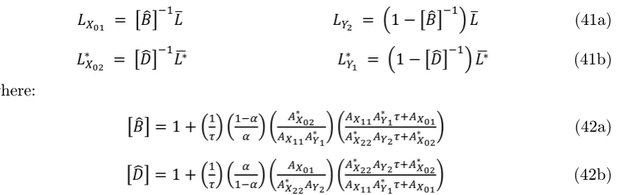
𝐿𝐿𝑋𝑋01 = �𝐵𝐵�� −1
𝐿𝐿� 𝐿𝐿𝑌𝑌2 = �1− �𝐵𝐵�� −1
� 𝐿𝐿� (41a)
𝐿𝐿𝑋𝑋∗02 = �𝐷𝐷�� −1
𝐿𝐿�∗ 𝐿𝐿𝑌𝑌 1
∗ = �1− �𝐷𝐷��−1� 𝐿𝐿�∗ (41b)
where:
�𝐵𝐵��= 1 +�1𝜏𝜏� �1−𝛼𝛼𝛼𝛼 � � 𝐴𝐴𝑋𝑋02∗ 𝐴𝐴𝑋𝑋11𝐴𝐴𝑌𝑌1∗ � �
𝐴𝐴𝑋𝑋11𝐴𝐴𝑌𝑌1∗ 𝜏𝜏+𝐴𝐴𝑋𝑋01
𝐴𝐴𝑋𝑋22∗ 𝐴𝐴𝑌𝑌2𝜏𝜏+𝐴𝐴∗𝑋𝑋02� (42a)
�𝐷𝐷��= 1 +�1𝜏𝜏� �1−𝛼𝛼𝛼𝛼 � � 𝐴𝐴𝑋𝑋01 𝐴𝐴𝑋𝑋22∗ 𝐴𝐴𝑌𝑌2� �
𝐴𝐴𝑋𝑋22∗ 𝐴𝐴𝑌𝑌2𝜏𝜏+𝐴𝐴𝑋𝑋02∗
𝐴𝐴𝑋𝑋11𝐴𝐴𝑌𝑌1∗ 𝜏𝜏+𝐴𝐴𝑋𝑋01� (42b)
Notice that, just as in autarky, because we assume that both sectors engage in indirect production, and the coordination cost is assumed to be the same across sectors, the coordination cost does not enter into the labour allocation across sectors, although the trade cost does. The coordination cost however does enter into the production function, resulting in a productivity cost and reducing the amount of each final good available
for consumption. As before, consumption of each good depends on each country’s
national income. Following the same steps as in Section 3.2, given the symmetry of the
model, the value of Home’s national income is:
𝑝𝑝𝑋𝑋1𝑄𝑄𝑋𝑋1 =
𝜏𝜏𝐴𝐴𝑋𝑋11𝐴𝐴𝑌𝑌1∗ +𝐴𝐴𝑋𝑋01
𝜏𝜏𝐴𝐴𝑋𝑋11𝐴𝐴𝑌𝑌1∗ [𝐵𝐵�] 𝐿𝐿� (43)
And Foreign’s national income is:
𝑝𝑝𝑋𝑋∗2𝑄𝑄𝑋𝑋∗2 =
𝜏𝜏𝐴𝐴𝑋𝑋22∗ 𝐴𝐴𝑌𝑌2+𝐴𝐴𝑋𝑋02∗
𝜏𝜏𝐴𝐴𝑋𝑋22∗ 𝐴𝐴𝑌𝑌2[𝐷𝐷�] 𝐿𝐿�∗ (44)
Home’s share of world income is therefore:
𝑆𝑆̂ =
𝜏𝜏𝐴𝐴𝑋𝑋11𝐴𝐴𝑌𝑌1∗ +𝐴𝐴𝑋𝑋01
𝜏𝜏𝐴𝐴𝑋𝑋11𝐴𝐴𝑌𝑌1∗ �𝐵𝐵�� 𝐿𝐿�
�𝜏𝜏𝐴𝐴𝑋𝑋11𝐴𝐴𝑌𝑌1∗ +𝐴𝐴𝑋𝑋01
𝜏𝜏𝐴𝐴𝑋𝑋11𝐴𝐴𝑌𝑌1∗ �𝐵𝐵�� 𝐿𝐿�� + �𝜏𝜏𝐴𝐴𝑋𝑋22
∗ 𝐴𝐴𝑌𝑌2+𝐴𝐴𝑋𝑋02∗
𝜏𝜏𝐴𝐴𝑋𝑋22∗ 𝐴𝐴𝑌𝑌2�𝐷𝐷�� 𝐿𝐿� �∗
(45)
Hence equilibrium consumption in the two countries is:
𝐶𝐶𝑋𝑋1 = 𝑆𝑆̂𝛽𝛽𝑇𝑇𝐴𝐴𝑋𝑋01�𝐵𝐵�� −1
𝐿𝐿� 𝐶𝐶𝑋𝑋∗1 = �1− 𝑆𝑆̂�𝜏𝜏𝛽𝛽𝑇𝑇𝐴𝐴𝑋𝑋01�𝐵𝐵�� −1
𝐿𝐿� (46a)
𝐶𝐶𝑋𝑋2 = 𝑆𝑆̂𝜏𝜏𝛽𝛽𝑇𝑇𝐴𝐴𝑋𝑋∗02�𝐷𝐷�� −1
𝐿𝐿�∗ 𝐶𝐶𝑋𝑋 2
∗ = �1− 𝑆𝑆̂�𝛽𝛽
𝑇𝑇𝐴𝐴𝑋𝑋∗02�𝐷𝐷�� −1
𝐿𝐿�∗ (46b)
The threshold values of 𝛽𝛽𝑇𝑇 are obtained by comparing these consumption levels with
consumption under international trade in final goods only (36a) and (36b):
𝛽𝛽�1𝑇𝑇 = 𝑆𝑆̂�𝐴𝐴𝛼𝛼𝛼𝛼𝐴𝐴𝑌𝑌1𝐴𝐴𝑋𝑋11[𝐵𝐵�]
𝑌𝑌1𝐴𝐴𝑋𝑋11+𝐴𝐴𝑋𝑋01� 𝛽𝛽�2𝑇𝑇 =
𝛼𝛼𝛼𝛼𝐴𝐴𝑌𝑌2∗ 𝐴𝐴𝑋𝑋22∗ [𝐷𝐷�]
𝑆𝑆̂�𝐴𝐴𝑌𝑌2∗ 𝐴𝐴𝑋𝑋22∗ +𝐴𝐴𝑋𝑋02∗ � (47)
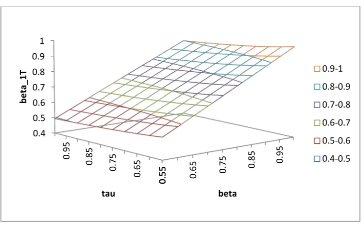
Values of 𝛽𝛽𝑇𝑇 greater than the threshold values mean that output with trade in both
[image:16.595.80.529.69.210.2]intermediate and final goods is larger than output with trade in final goods alone. Figure 1 shows that the threshold values depend positively on the domestic
16
the trade cost 𝜏𝜏; the relationship with 𝛽𝛽 is a general result, while the relationship with
[image:17.595.116.481.148.375.2]𝜏𝜏 depends on other parameter values6.
Figure 1: Threshold values of 𝛽𝛽1𝑇𝑇 as a function of 𝛽𝛽 and 𝜏𝜏.
3.5 A history of the international organisation of production
The previous subsections have shown how production is organised in the world economy depending on the coordination and trade costs that exist. In this subsection we consider what happens as both trade and coordination costs decrease over time. The outcomes depend in a relatively complex way on these trade and coordination costs; hence we offer here an example of the parameter values under which different configurations exist.
Suppose initially that both types of costs are very high; for example, 𝛽𝛽 =𝜏𝜏 = 0.4 and
𝛽𝛽𝑇𝑇 = 0.3. Whilst these may appear to be very large trade costs (equivalent to a trade friction of 150%), this is not out of line with the figures quoted in Anderson and van Wincoop (2004), who suggest a total trade barrier of 170% in developed countries. With such high costs, it is not beneficial to engage in international trade, or indeed to
engage in domestic indirect production. This is the situation with Henry Ford’s
6 This can also be seen by substituting (42a), (42b) and (45) into (47). Since 𝛽𝛽 does not enter into �𝐵𝐵��,
�𝐷𝐷�� or �𝑆𝑆̂�, there is a direct relationship between 𝛽𝛽 and 𝛽𝛽�1𝑇𝑇 and 𝛽𝛽�2𝑇𝑇. However, 𝜏𝜏 enters into all of �𝐵𝐵��,
�𝐷𝐷�� and �𝑆𝑆̂�, and these appear in both the numerator and denominator of 𝛽𝛽�1𝑇𝑇 and 𝛽𝛽�2𝑇𝑇, so 𝜏𝜏 has a complicated relationship with 𝛽𝛽�1𝑇𝑇 and 𝛽𝛽�2𝑇𝑇.
0.
55
0.
65
0.
75
0.
85
0.
95
0.4 0.5 0.6 0.7 0.8 0.9 1
0.
55 0.65 0.75 0. 85 0.95
tau
bet
a_
1T
beta
17
monolithic factory: firms produce final goods directly from raw materials, and there is no international trade.
What happens next depends on whether trade costs decrease faster than coordination
costs or vice versa. In the former case, suppose that 𝛽𝛽 = 0.4, 𝛽𝛽𝑇𝑇 = 0.3 as before, and 𝜏𝜏 increases to 0.5. This is sufficient to ensure that international trade in final goods with direct production is the most beneficial outcome. In this case Home will specialise in
𝑋𝑋1 and export it to Foreign in exchange for imports of 𝑋𝑋2. On the other hand, if
coordination costs decrease faster than trade costs, then autarky with indirect
production will occur, for instance if 𝛽𝛽𝑇𝑇 = 0.3, and 𝜏𝜏= 0.4 as before, then 𝛽𝛽= 0.593 is sufficient to obtain this outcome. Therefore, industries in which trade costs are relatively low compared to coordination costs will be engaged in international trade, whereas industries in which trade costs are relatively high will engage in domestic indirect production.
As both trade and coordination costs continue to fall, production begins to take place indirectly, although only international trade in final goods continues to occur. For
example, this occurs if 𝛽𝛽𝑇𝑇 = 0.3 as before, and 𝛽𝛽=𝜏𝜏 = 0.625. Therefore, as trade and coordination costs fall, countries may actually become less specialised as they move from international trade with direct production to international trade with indirect production. And finally, when the cost of coordinating imported intermediate products is sufficiently small relative to the cost of coordinating domestically produced
intermediate products (𝛽𝛽𝑇𝑇 is sufficiently close to 𝛽𝛽), countries will trade both
intermediate and final goods, specialising in the production of intermediates and final goods in which they have a comparative advantage. This is the production structure of the Apple iPod as discussed in the Introduction. Given the parameters assumed
above, an example of this occurring is when 𝛽𝛽 =𝜏𝜏 = 0.65, and 𝛽𝛽𝑇𝑇 = 0.62.
If inputs are defined as being in the same industry as the final good it is used in, then
trade will be intra-industry in nature: Home exports 𝑋𝑋1 and 𝑌𝑌2 in exchange for imports
of 𝑋𝑋2 and 𝑌𝑌1. Therefore, intra-industry trade can occur only when the cost of
18
the existence of such standards (see for example Clougherty and Grajek, 2008). A similar role may exist for business networks (see for example Rauch, 2001).
4
Conclusions
This paper develops a simple model of international trade with 2 countries, 2 final goods, 2 intermediate goods, and one factor of production. The objective is to explore the structure of production that emerges. Both domestic and foreign outsourcing lead to productivity gains. Despite the simple setup, the model allows for many possible outcomes, depending on the cost of international trade and the cost of coordinating intermediate inputs. When both trade and coordination costs are very high, not only is there no international trade, but firms engage in direct production of final goods (that is, they do not make use of intermediate inputs produced outside the firm). As coordination costs fall, indirect production of final goods occurs with the use of domestic intermediate inputs, while as trade costs fall, international trade in final goods occurs. Finally, when coordination costs for imported intermediates are not too large relative to the coordination costs of domestically produced intermediates, international trade occurs in both intermediate and final goods, and production occurs indirectly through the use of imported intermediates. Hence as trade costs decrease, the international structure of production endogenously becomes more fragmented, and countries become more inter-dependent.
19
Acknowledgements
Thanks to the editor, Hamid Beladi, an anonymous referee, and seminar participants at Lancaster University for helpful suggestions. The author is responsible for any errors and omissions. This research did not receive any specific grant from funding agencies in the public, commercial, or not-for-profit sectors.
References
Amiti, Mary and Shang-Jin Wei (2009), “Service offshoring and productivity: Evidence
from the US”, The World Economy 32(2): 203-220.
Anderson, James E. and Eric van Wincoop (2004), “Trade costs”, Journal of Economic
Literature 42(3): 691-751.
Antras, Pol (2003), “Firms, contracts, and trade structure”, Quarterly Journal of
Economics 118(4): 1375-1418.
Antras, Pol and Elhanan Helpman (2004), “Global sourcing”, Journal of Political
Economy 112(3): 552-580.
Baldwin, Richard (2016), The great convergence, Harvard, MA, Harvard University Press.
Brown, Clair and Greg Linden (2005), “Offshoring in the semiconductor industry: A
historical perspective”, Brookings Trade Forum, 279-333.
Clougherty, Joseph A. and Michal Grajek (2008), “The impact of ISO 9000 diffusion
on trade and FDI: A new institutional analysis”, Journal of International Business
Studies 39(4): 613-633.
Eaton, Jonathan and Samuel Kortum (2002), “Technology, geography, and trade”,
Econometrica 70(5): 1741-1779.
Ethier, Wilfred J. (1982), “National and international returns to scale in the modern
theory of international trade”, American Economic Review 72(3): 389-405.
Feenstra, Robert C. (2009), Offshoring in the global economy, Cambridge, MA, MIT Press.
Feenstra, Robert C and Gordon H. Hanson (1996), “Foreign investment, outsourcing
and relative wages”, in Robert C. Feenstra, Gene M. Grossman and Douglas A. Irwin
(eds.), The political economy of trade policy: Papers in honor of Jagdish Bhagwati,
20
Feenstra, Robert C. and Gordon H. Hanson (1997), “Foreign direct investment and
relative wages: Evidence from Mexico’s maquiladoras”, Journal of International
Economics 42(3-4): 371-393.
Fort, Teresa C. (2017), “Technology and production fragmentation: Domestic versus
foreign sourcing”, Review of Economic Studies 84(2): 650-687.
Fujimoto, Takahiro and Yoshinori Shiozawa (2011a), “Inter and intra company
competition in the age of global competition: A micro and macro interpretation of
Ricardian trade theory”, Evolutionary and Institutional Economics Review 8(1): 1-37.
Fujimoto, Takahiro and Yoshinori Shiozawa (2011b), “Inter and intra company
competition in the age of global competition: A micro and macro interpretation of
Ricardian trade theory”, Evolutionary and Institutional Economics Review 8(2):
193-231.
Gorg, Holger, Aoife Hanley and Eric Strobl (2008), “Productivity effects of
international outsourcing: Evidence from plant-level data”, Canadian Journal of
Economics 41(2): 670-688.
Gross, Daniel (1997), Forbes greatest business stories, New York, John Wiley & Sons.
Grossman, Gene M. and Elhanan Helpman (2002), “Integration versus outsourcing in
industry equilibrium”, Quarterly Journal of Economics 117(1): 85-120.
Grossman, Gene M. and Esteban Rossi-Hansberg (2008), “Trading tasks: A simple
theory of offshoring”, American Economic Review 98(5): 1978-1997.
Grubel, Herbert G. And Peter J. Lloyd (1975), Intra-industry trade: The theory and measurement of international trade in differentiated products, New York, Wiley.
Helpman, Elhanan, Marc J. Melitz and Stephen R. Yeaple (2004), “Export versus FDI
with heterogeneous firms”, American Economic Review 94(1): 300-316.
Houseman, Susan (2007), “Outsourcing, offshoring and productivity measurement in
United States manufacturing”, International Labour Review 146(1-2): 61-80.
Jones, Ronald W. (2000), Globalization and the theory of input trade, Cambridge, MA, MIT Press.
Jones, Ronald W. and Henryk Kierzkowski (1990), “The role of services in production
and international trade: A theoretical framework”, in Ronald W. Jones and Anne O.
21
Knittel, Christopher and Victor Stango (2012), “The productivity benefits of IT
outsourcing”, mimeo, MIT.
Linden, Greg, Kenneth L. Kraemer and Jason Dedrick (2007), “Who captures value in
a global innovation system? The case of Apple’s iPod”, Communications of the ACM
52(3): 140-144.
Mankiw, N. Gregory and Phillip Swagel (2006), “The politics and economics of offshore
outsourcing”, Journal of Monetary Economics 53(5): 1027-1056.
Melitz, Marc J. (2003), “The impact of trade on intra-industry reallocations and
aggregate industry productivity”, Econometrica 71(6): 1695-1725.
Olsen, Karsten Bjerring (2006), “Productivity impacts of offshoring and outsourcing:
A review”, STI Working Paper 2006/1, OECD.
Rauch, James E. (2001), “Business and social networks in international trade”, Journal
of Economic Literature 39(4): 1177-1203.
Ricardo, David (1817), On the principles of political economy and taxation, London, John Murray.
Rodriguez-Clare, Andres (2010), “Offshoring in a Ricardian world”, American
Economic Journal: Macroeconomics 2(2): 227-258.
Samuelson, Paul A. (2001), “A Ricardo-Sraffa paradigm comparing gains from trade
in inputs and finished goods”, Journal of Economic Literature 39(4): 1204-1214.
Sanyal, Kalyan (1983), “Trade in raw materials in a simple Ricardian model”, Institute
for International Economic Studies, Seminar Paper 233.
Sanyal, Kalyan and Ronald W. Jones (1982), “The theory of trade in middle products”,
American Economic Review 72(1): 16-31.
Shiozawa, Yoshinori (2007), “A new construction of Ricardian trade theory – A
many-country, many-commodity case with intermediate goods and choice of production
techniques”, Evolutionary and Institutional Economics Review 3(2): 141-187.
Shiozawa, Yoshinori (2009), “Samuelson’s implicit criticism against Sraffa and the
Sraffians and two other questions”, Kyoto Economic Review 78(1): 19-37.
Sraffa, Piero (1960), Production of commodities by means of commodities, Cambridge, Cambridge University Press.
Sturgeon, Timothy J. (2002), “Modular production networks: A new American model
22
US Government Accountability Office (2006), “Offshoring: US Semiconductor and
software industries increasingly produce in China and India”, US Government
Accountability Office Report to Congressional Committees 06-423.
Yi, Kei-Mu (2003), “Can vertical specialization explain the growth of world trade?”,
23
Appendix A: Equilibrium conditions with international trade in final goods
only
The equilibrium conditions when international trade is allowed in final goods only are as follows:
𝑝𝑝𝑋𝑋1 = 𝑝𝑝𝑋𝑋∗1 =
𝑤𝑤�𝐴𝐴𝑋𝑋11𝐴𝐴𝑌𝑌1+𝐴𝐴𝑋𝑋01�
𝐴𝐴𝑋𝑋01𝐴𝐴𝑋𝑋11𝐴𝐴𝑌𝑌1 𝑝𝑝𝑋𝑋2 =𝑝𝑝𝑋𝑋∗2 =
𝑤𝑤∗�𝐴𝐴𝑋𝑋22∗ 𝐴𝐴𝑌𝑌2∗ +𝐴𝐴𝑋𝑋02∗ �
𝐴𝐴𝑋𝑋02∗ 𝐴𝐴𝑋𝑋22∗ 𝐴𝐴𝑌𝑌2∗ (A1)
𝑝𝑝𝑋𝑋1 𝑝𝑝𝑋𝑋2 = �
𝐴𝐴𝑋𝑋02∗ 𝐴𝐴𝑋𝑋22∗ 𝐴𝐴𝑌𝑌2∗ 𝐴𝐴𝑋𝑋01𝐴𝐴𝑋𝑋11𝐴𝐴𝑌𝑌1� �
𝐴𝐴𝑋𝑋11𝐴𝐴𝑌𝑌1+𝐴𝐴𝑋𝑋01 𝐴𝐴𝑋𝑋22∗ 𝐴𝐴𝑌𝑌2∗ +𝐴𝐴𝑋𝑋02∗ �=
𝛼𝛼 1−𝛼𝛼�
𝐶𝐶𝑋𝑋2
𝐶𝐶𝑋𝑋1� (A2)
𝐶𝐶𝑋𝑋2 𝐶𝐶𝑋𝑋1 =
𝐴𝐴𝑋𝑋02∗ 𝐿𝐿𝑋𝑋02∗ 𝐴𝐴𝑋𝑋01𝐿𝐿𝑋𝑋01 =
𝐴𝐴𝑋𝑋22∗ 𝐴𝐴𝑌𝑌2∗ 𝐿𝐿𝑌𝑌2∗
𝐴𝐴𝑋𝑋11𝐴𝐴𝑌𝑌1𝐿𝐿𝑌𝑌1 (A3)
𝐿𝐿𝑋𝑋02∗ 𝐿𝐿𝑋𝑋01 = �
1−𝛼𝛼 𝛼𝛼 � �
𝐴𝐴𝑋𝑋22∗ 𝐴𝐴𝑌𝑌2∗ 𝐴𝐴𝑋𝑋11𝐴𝐴𝑌𝑌1� �
𝐴𝐴𝑋𝑋11𝐴𝐴𝑌𝑌1+𝐴𝐴𝑋𝑋01
𝐴𝐴𝑋𝑋22∗ 𝐴𝐴𝑌𝑌2∗ +𝐴𝐴𝑋𝑋02∗ � (A4)
𝐿𝐿𝑌𝑌2∗ 𝐿𝐿𝑌𝑌1 = �
1−𝛼𝛼 𝛼𝛼 � �
𝐴𝐴𝑋𝑋02∗ 𝐴𝐴𝑋𝑋01� �
𝐴𝐴𝑋𝑋11𝐴𝐴𝑌𝑌1+𝐴𝐴𝑋𝑋01
𝐴𝐴𝑋𝑋22∗ 𝐴𝐴𝑌𝑌2∗ +𝐴𝐴𝑋𝑋02∗ � (A5)
𝐴𝐴𝑋𝑋01𝐿𝐿𝑋𝑋01 = 𝐴𝐴𝑋𝑋11𝐴𝐴𝑌𝑌1𝐿𝐿𝑌𝑌1 ↔ 𝐿𝐿𝑋𝑋01 =
𝐴𝐴𝑋𝑋11𝐴𝐴𝑌𝑌1
𝐴𝐴𝑋𝑋01 𝐿𝐿𝑌𝑌1 (A6)
𝐴𝐴∗𝑋𝑋02𝐿𝐿∗𝑋𝑋02 = 𝐴𝐴𝑋𝑋∗22𝐴𝐴∗𝑌𝑌2𝐿𝐿∗𝑌𝑌2 ↔ 𝐿𝐿∗𝑋𝑋02 =
𝐴𝐴𝑋𝑋22∗ 𝐴𝐴𝑌𝑌2∗
𝐴𝐴𝑋𝑋02∗ 𝐿𝐿∗𝑌𝑌2 (A7)
𝐿𝐿𝑋𝑋01+ 𝐿𝐿𝑌𝑌1 = 𝐿𝐿� 𝐿𝐿∗𝑋𝑋02+ 𝐿𝐿∗𝑌𝑌2 = 𝐿𝐿�∗ 𝑤𝑤 =𝑤𝑤∗ (A8)
Appendix B: Equilibrium conditions with international trade in both
intermediate and final goods
The equilibrium conditions when international trade is allowed in both intermediate and final goods are as follows:
𝑝𝑝𝑋𝑋1 = 𝑝𝑝𝑋𝑋∗1 =
𝑤𝑤𝐴𝐴𝑋𝑋11𝐴𝐴𝑌𝑌1∗ +𝑤𝑤∗𝐴𝐴𝑋𝑋01
𝐴𝐴𝑋𝑋01𝐴𝐴𝑋𝑋11𝐴𝐴𝑌𝑌1∗ (B1)
𝑝𝑝𝑋𝑋2 = 𝑝𝑝𝑋𝑋∗2 = 𝑤𝑤∗𝐴𝐴
𝑋𝑋22
∗ 𝐴𝐴
𝑌𝑌2+𝑤𝑤𝐴𝐴𝑋𝑋02∗
𝐴𝐴𝑋𝑋02∗ 𝐴𝐴𝑋𝑋22∗ 𝐴𝐴𝑌𝑌2 (B2)
𝑝𝑝𝑋𝑋1 𝑝𝑝𝑋𝑋2 = �
𝐴𝐴𝑋𝑋02∗ 𝐴𝐴𝑌𝑌2𝐴𝐴𝑋𝑋22∗ 𝐴𝐴𝑋𝑋01𝐴𝐴𝑌𝑌1∗ 𝐴𝐴𝑋𝑋11� �
𝐴𝐴𝑋𝑋11𝐴𝐴𝑌𝑌1∗ +𝐴𝐴𝑋𝑋01 𝐴𝐴𝑋𝑋22∗ 𝐴𝐴𝑌𝑌2+𝐴𝐴𝑋𝑋02∗ �=
𝛼𝛼 1−𝛼𝛼�
𝐶𝐶𝑋𝑋2
𝐶𝐶𝑋𝑋1� (B3)
𝐶𝐶𝑋𝑋2 𝐶𝐶𝑋𝑋1 =
𝐴𝐴𝑋𝑋02∗ 𝐿𝐿∗𝑋𝑋02 𝐴𝐴𝑋𝑋01𝐿𝐿𝑋𝑋01 =
𝐴𝐴𝑋𝑋22∗ 𝐴𝐴𝑌𝑌2𝐿𝐿𝑌𝑌2
𝐴𝐴𝑋𝑋11𝐴𝐴𝑌𝑌1∗ 𝐿𝐿𝑌𝑌1∗ (B4)
𝐿𝐿𝑋𝑋02∗ 𝐿𝐿𝑋𝑋01 = �
1−𝛼𝛼 𝛼𝛼 � �
𝐴𝐴𝑌𝑌2𝐴𝐴𝑋𝑋22∗ 𝐴𝐴𝑌𝑌1∗ 𝐴𝐴
𝑋𝑋11� �
𝐴𝐴𝑋𝑋11𝐴𝐴𝑌𝑌1∗ +𝐴𝐴𝑋𝑋01 𝐴𝐴𝑋𝑋22∗ 𝐴𝐴
𝑌𝑌2+𝐴𝐴𝑋𝑋02∗ � (B5)
𝐿𝐿𝑌𝑌2 𝐿𝐿𝑌𝑌1∗ = �
1−𝛼𝛼 𝛼𝛼 � �
𝐴𝐴𝑋𝑋02∗ 𝐴𝐴𝑋𝑋01� �
𝐴𝐴𝑋𝑋11𝐴𝐴𝑌𝑌1∗ +𝐴𝐴𝑋𝑋01
24
𝐴𝐴𝑋𝑋01𝐿𝐿𝑋𝑋01 = 𝐴𝐴𝑋𝑋11𝐴𝐴∗𝑌𝑌1𝐿𝐿∗𝑌𝑌1 ↔ 𝐿𝐿𝑋𝑋01=
𝐴𝐴𝑋𝑋11𝐴𝐴𝑌𝑌1∗
𝐴𝐴𝑋𝑋01 𝐿𝐿∗𝑌𝑌1 (B7)
𝐴𝐴𝑋𝑋∗02𝐿𝐿∗𝑋𝑋02 = 𝐴𝐴𝑋𝑋∗22𝐴𝐴𝑌𝑌2𝐿𝐿𝑌𝑌2 ↔ 𝐿𝐿∗𝑋𝑋02=
𝐴𝐴𝑋𝑋22∗ 𝐴𝐴𝑌𝑌2
𝐴𝐴𝑋𝑋02∗ 𝐿𝐿𝑌𝑌2 (B8)
𝐿𝐿𝑋𝑋01+ 𝐿𝐿𝑌𝑌2 = 𝐿𝐿� 𝐿𝐿∗𝑋𝑋02+ 𝐿𝐿∗𝑌𝑌1 = 𝐿𝐿�∗ 𝑤𝑤 =𝑤𝑤∗ (B9)
Appendix C: Equilibrium conditions with trade and coordination costs
The equilibrium conditions when trade in both intermediate and final goods is allowed
in the presence of trade and coordination costs are (setting 𝑤𝑤 = 𝑤𝑤∗):
𝑝𝑝𝑋𝑋1 =𝜏𝜏𝑝𝑝𝑋𝑋∗1 =
𝑤𝑤�𝐴𝐴𝑋𝑋11𝐴𝐴𝑌𝑌1∗ 𝜏𝜏+𝐴𝐴𝑋𝑋01�
𝛼𝛼𝑇𝑇𝜏𝜏𝐴𝐴𝑋𝑋01𝐴𝐴𝑋𝑋11𝐴𝐴𝑌𝑌1∗ (C1)
𝑝𝑝𝑋𝑋2 = 𝑝𝑝𝑋𝑋2∗
𝜏𝜏 =
𝑤𝑤�𝐴𝐴𝑋𝑋22∗ 𝐴𝐴𝑌𝑌2𝜏𝜏+𝐴𝐴∗𝑋𝑋02�
𝛼𝛼𝑇𝑇𝜏𝜏2𝐴𝐴𝑋𝑋02∗ 𝐴𝐴𝑋𝑋22∗ 𝐴𝐴𝑌𝑌2 (C2)
𝑝𝑝𝑋𝑋1 𝑝𝑝𝑋𝑋2 = 𝜏𝜏 �
𝐴𝐴𝑋𝑋02∗ 𝐴𝐴𝑌𝑌2𝐴𝐴𝑋𝑋22∗ 𝐴𝐴𝑋𝑋01𝐴𝐴𝑌𝑌1∗ 𝐴𝐴𝑋𝑋11� �
𝐴𝐴𝑋𝑋11𝐴𝐴𝑌𝑌1∗ 𝜏𝜏+𝐴𝐴𝑋𝑋01 𝐴𝐴𝑋𝑋22∗ 𝐴𝐴𝑌𝑌2𝜏𝜏+𝐴𝐴𝑋𝑋02∗ �=
𝛼𝛼 1−𝛼𝛼�
𝐶𝐶𝑋𝑋2
𝐶𝐶𝑋𝑋1� (C3)
𝐶𝐶𝑋𝑋2 𝐶𝐶𝑋𝑋1 =
𝜏𝜏𝐴𝐴𝑋𝑋02∗ 𝐿𝐿∗𝑋𝑋02 𝐴𝐴𝑋𝑋01𝐿𝐿𝑋𝑋01 =
𝜏𝜏𝐴𝐴𝑋𝑋22∗ 𝐴𝐴𝑌𝑌2𝐿𝐿𝑌𝑌2
𝐴𝐴𝑋𝑋11𝐴𝐴𝑌𝑌1∗ 𝐿𝐿𝑌𝑌1∗ (C4)
𝐿𝐿∗𝑋𝑋02 𝐿𝐿𝑋𝑋01 = �
1−𝛼𝛼 𝛼𝛼 � �
𝐴𝐴𝑌𝑌2𝐴𝐴𝑋𝑋22∗ 𝐴𝐴𝑌𝑌1∗ 𝐴𝐴𝑋𝑋11� �
𝐴𝐴𝑋𝑋11𝐴𝐴𝑌𝑌1∗ 𝜏𝜏+𝐴𝐴𝑋𝑋01
𝐴𝐴𝑋𝑋22∗ 𝐴𝐴𝑌𝑌2𝜏𝜏+𝐴𝐴𝑋𝑋02∗ � (C5)
𝐿𝐿𝑌𝑌2 𝐿𝐿∗𝑌𝑌1 = �
1−𝛼𝛼 𝛼𝛼 � �
𝐴𝐴𝑋𝑋02∗ 𝐴𝐴𝑋𝑋01� �
𝐴𝐴𝑋𝑋11𝐴𝐴𝑌𝑌1∗ 𝜏𝜏+𝐴𝐴𝑋𝑋01
𝐴𝐴𝑋𝑋22∗ 𝐴𝐴𝑌𝑌2𝜏𝜏+𝐴𝐴∗𝑋𝑋02� (C6)
𝛽𝛽𝑇𝑇𝐴𝐴𝑋𝑋01𝐿𝐿𝑋𝑋01 = 𝛽𝛽𝑇𝑇𝜏𝜏𝐴𝐴𝑋𝑋11𝐴𝐴𝑌𝑌∗1𝐿𝐿∗𝑌𝑌1 ↔ 𝐿𝐿𝑋𝑋01 =
𝜏𝜏𝐴𝐴𝑋𝑋11𝐴𝐴𝑌𝑌1∗
𝐴𝐴𝑋𝑋01 𝐿𝐿∗𝑌𝑌1 (C7)
𝛽𝛽𝑇𝑇𝐴𝐴𝑋𝑋∗02𝐿𝐿∗𝑋𝑋02= 𝛽𝛽𝑇𝑇𝜏𝜏𝐴𝐴∗𝑋𝑋22𝐴𝐴𝑌𝑌2𝐿𝐿𝑌𝑌2 ↔ 𝐿𝐿∗𝑋𝑋02 =
𝜏𝜏𝐴𝐴𝑋𝑋22∗ 𝐴𝐴𝑌𝑌2
𝐴𝐴𝑋𝑋02∗ 𝐿𝐿𝑌𝑌2 (C8)
𝐿𝐿𝑋𝑋01+ 𝐿𝐿𝑌𝑌2 = 𝐿𝐿� 𝐿𝐿∗𝑋𝑋02+ 𝐿𝐿∗𝑌𝑌1 = 𝐿𝐿�∗ (C9)
Appendix D: Comparison with Samuelson
’
s (2001) results
The equivalent parameter values used in Samuelson’s (2001) paper are: