warwick.ac.uk/lib-publications
Manuscript version: Author’s Accepted Manuscript
The version presented in WRAP is the author’s accepted manuscript and may differ from the published version or Version of Record.
Persistent WRAP URL:
http://wrap.warwick.ac.uk/110994
How to cite:
Please refer to published version for the most recent bibliographic citation information. If a published version is known of, the repository item page linked to above, will contain details on accessing it.
Copyright and reuse:
The Warwick Research Archive Portal (WRAP) makes this work by researchers of the University of Warwick available open access under the following conditions.
© 2018 Elsevier. Licensed under the Creative Commons Attribution-NonCommercial-NoDerivatives 4.0 International http://creativecommons.org/licenses/by-nc-nd/4.0/.
Publisher’s statement:
Please refer to the repository item page, publisher’s statement section, for further information.
A study of magnetostriction mechanism of EMAT on
low-carbon steel at high temperature
Weiping Ren 1, Ke Xu 1,*, Steve Dixon 2 and Chu Zhang 1
1 Collaborative Innovation Center of Steel Technology, University of Science and Technology Beijing, Beijing 100083, China
2 Department of Physics, University of Warwick, Coventry CV4 7AL, UK; S.M.Dixon@warwick.ac.uk (S.D.)
* Correspondence: xuke@ustb.edu.cn; Tel.: +86-10-6233-2159
Abstract
The Electromagnetic acoustic transducer (EMAT) is used in a number of non-destructive testing applications [1-5]. The EMAT's operation is principally based on one of two mechanisms;
the Lorenz force and magnetostriction mechanism [6-9]. The magnetostriction mechanism of an EMAT at elevated temperatures is reported in this paper. An optimized model is developed to
describe the magnetostriction of polycrystalline iron, which is based on Brown’s magnetic domain wall movement model[10] and Lee’s magnetic domain rotation model [11]. The magnetostriction curves of polycrystalline iron for the temperature range 300 K to 900 K are predicted, which
reveal that the saturated magnetostriction coefficient changes from to approximately
. A non-linear, isotropic magnetostriction, finite element model is developed to simulate
the Lamb waves generated in 4 mm thick steel plate by an EMAT, and the results show that the amplitude of S0 Lamb wave is greatly enhanced with an increase of temperature. In the experiments, a magnetostriction-based EMAT is used to generate Lamb waves in 4 mm thick steel
plate. Experimental measurements verify that the contribution of the magnetostriction mechanism on steel rises as temperature increases in the range 298 K to 873 K, while the contribution to
ultrasonic generation from the Lorenz force mechanism decreases, as expected.
Key words
Electromagnetic acoustic transducer, magnetostriction mechanism, high temperature, finite
element model, low-carbon steel
1. Introduction
Electromagnetic acoustic transducers (EMATs) are used in non-destructive testing (NDT) as they offer several benefits including their non-contacting nature and their ability to generate and detect a range of wave modes [7, 12, 13] that are difficult to achieve using conventional
transducers. The non-contact nature of EMATs makes them suitable for NDT applications where the object under test is at an elevated temperature or is moving [14-18]. EMATs have poor
electro-mechanical efficiency as either generators or detectors and can have complicated coupling mechanisms for ferromagnetic materials, where both magnetoelastic and Lorentz mechanisms contribute to transduction. Research has been undertaken in an attempt to improve the efficiency
of the EMAT and better understand the physics behind the coupling mechanisms involved [7, 8, 19-23]. In operating on non-ferromagnetic materials, the EMAT has only Lorentz force
mechanisms to consider. In ferromagnetic materials, magnetostriction and magnetisation mechanisms must also be considered [7, 8]. Research on the quantization of the Lorentz force mechanism and magnetostriction mechanism has shown that, for the conventional EMAT that can
generation or detection of ultrasonic waves. Certain EMAT designs can also make
magnetostriction the major contributor [26] to ultrasonic generation by increasing the lift-off of a coil-only generator.
An EMAT generates ultrasonic waves in the sample's electromagnetic skin-depth directly, while a contacting piezoelectric ultrasound probe generates ultrasound waves in the active piezoelectric element inside the probe, which then propagates through the probe into the sample
[27]. Therefore, the efficiency of EMATs is related to the EMAT lift-off from the surface of the sample, the EMAT design and the physical properties of the sample, including electrical
conductivity, magnetic permeability, Young's modulus, etc., which can be significantly affected by the temperature [28-30]. In high temperature applications, the efficiency of EMAT as a generator or detector usually reduces drastically, due to the reduction of Lorentz force, linked to a decrease
in the electrical conductivity of the sample [17, 18, 22].
This paper focuses on the contribution of the magnetostriction mechanism to the EMAT
when a low-carbon steel sample is at elevated temperature. A magnetostriction model is developed to predict the magnetostriction curves of polycrystalline iron at different temperatures. A 2-D,
non-linear, isotropic magnetisation finite element (FE) model is also built, which is used to simulate and analyse the process of excitation by the EMAT in the time domain. In addition, series experimental measurements are conducted to validate the simulation results.
2. Theory
2.1 Magnetostrictive effect.
In the magnetostrictive effect, also known as the Joule effect, strain is induced in a sample by the application of a magnetic field. The atomic orbital moment and spin magnetic exchange
interaction changes, resulting in changes in the magneto-elastic properties of the sample. In the direction of the lowest magneto-elastic energy, the maximum displacement occurs between
adjacent atoms, causing strain in a region called the magnetic domain. For cubic crystals, the
magnetostriction coefficient of a single domain can be obtained from
where, ( =1,2,3) are the direction cosines of the direction of measurement referenced to the
crystallographic axes, and are the direction cosines of the direction of spontaneous
magnetisation referenced to the crystallographic axes. The parameters and are the spontaneous magnetostriction coefficients along the [100] and [111] crystal axes respectively. At
room temperature [31], the values of these two coefficients are and
.
Due to the relatively high energy of a single magnetic domain body, the magnetic material
naturally arranges itself into massive smaller magnetic domains to minimise the free energy of the system, whether the material is single crystal or polycrystal sample [29]. The crystallographic axes
directions of single crystal are completely defined, whilst for a polycrysalline sample the individual grains are usually almost randomly orientated with respect to each other, although working metals can produce some amount of anisotropy. Therefore, the magnetostrictive
behavior. Polycrystalline alloys of iron are the most widely used metals in engineering and are the
most common targets samples for an EMAT. Therefore, polycrystalline iron is the main focus of this paper.
H H H
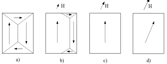
[image:4.595.172.445.134.239.2]a) b) c) d)
Fig. 1 Magnetisation process of a grain. The arrows inside the grain represent the spontaneous magnetisation direction of the magnetic domains. Without the application of an
external magnetic field (a) the net magnetisation of the sample is zero. As a small external field is applied (b). At a higher applied field (c), the magnetic domain wall movement is completed, until
finally at an even higher level of applied magnetic field (d) the magnetisation direction of the magnetic domain rotates to tend to align with the applied field.
Due to the presence of the magnetic domains, magnetic materials that have been demagnetised or that have no barriers to magnetic domain wall motion do not show magnetism
and magnetostriction whenno external magnetic field is applied. However, if an external magnetic
field H exists, those magnetic domains with a smaller angle between the direction of spontaneous
magnetisation and the external magnetic field become larger, and vice versa, which is achieved by
the movement of magnetic domain walls. When the external magnetic field continues to increase, the magnetic domains rotate, trying to make the angle between the direction of spontaneous
magnetisation of the magnetic domains and the external magnetic field direction smaller, as shown in Fig. 1. In the phase of magnetic domain wall movement, assuming that the magnetisation directions of these magnetic domains are random in a polycrystalline sample, the change in the
macroscopic magnetostriction can be obtained by calculating the average of the magnetostriction changes of these domains. It is necessary in principle, to know the number, size and shape of each
domain as well as the direction of its magnetisation vector. This information is usually not available for real samples, and instead it is usually assumed that the number of domains is so great that the material may be regarded as being in a state of uniform stress. In this case, the mean strain
is simply the volume average of the individual strains. Only the distribution of the direction of the
domain vectors need then be known. This may be characterized by a distribution function , so
that the mean magnetostriction can be given by
where, is an elementary solid angle [11].
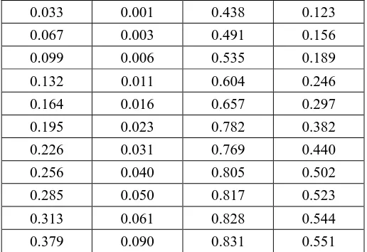
Table 1. Magnetostriction coefficients contributed by the domain wall movement.
0.033 0.001 0.438 0.123
0.067 0.003 0.491 0.156
0.099 0.006 0.535 0.189
0.132 0.011 0.604 0.246
0.164 0.016 0.657 0.297
0.195 0.023 0.782 0.382
0.226 0.031 0.769 0.440
0.256 0.040 0.805 0.502
0.285 0.050 0.817 0.523
0.313 0.061 0.828 0.544
0.379 0.090 0.831 0.551
Brown considers that the distribution of the function conforms to the Boltzmann
distribution and thus yields the magnetostriction coefficients [10], as shown in table 1. Note that in
table 1, the magnetisation rate is the ratio of the magnetisation to the saturation
magnetisation . As a supplement, Lee gives a magnetostriction model for the magnetic domain
rotation phase [11]. The easy magnetisation axis of the iron cubic crystal is [100], and because of the symmetry of a cube, the relative position between the directions of the external magnetic field
and the spontaneous magnetisation is limited to a triangle on a unit sphere as shown in Fig. 2. In the spherical coordinate system, the direction of is represented by and , the
direction of is represented by and , then:
(3)
where, indicates the degree of magnetic domain rotation, and = 1 represents magnetic
saturation. The parameter can be obtained by the area integral of the triangle:
where, is given by . For a fixed value of , the corresponding average
magnetisation rate can be obtained.
For magnetostriction, expressing and in terms of , and , , from the
equations (1) and (3) one obtains:
Both of these expressions can be averaged using the same method as used to obtain . The analytic solution of the integral may be difficult to acquire, but the numerical solution can be
[image:5.595.169.427.72.249.2]by assuming a series of values for A. So, the magnetostriction curve of polycrystalline iron can be
obtained by combining magnetic domain wall movement and magnetic domain rotation, as shown in Fig. 3. However, the results are quite different from those obtained from the experiment[11],
and only agree with them when the magnetisation rate is low or high.
[001]
[010] [100]
[110] [111]
Is
[image:6.595.226.393.140.285.2]H
Fig. 2. The relative position between the direction of the external magnetic field and the
direction of the spontaneous magnetisation . The axes [001], [010], [100] are the three axes of
cartesian coordinate system, and the triangle is part of the unit sphere.
η
c λsλc
Fig. 3. The magnetostriction curves of polycrystal iron that from Brown’s and Lee’s models and that from Yamasaki’s measurement[32].
2.2 Model optimization
Lee's magnetic domain rotation model is based on the assumption that the magnetic domain
wall movement has been completed before the magnetic moment start to align with the applied field. However, these two processes are actually occurring at the same time in realistic samples
[10], which mainly cause this divergence between the experiment results and the prediction. Usually, defects and impurities in the crystal structure can form potential energy barriers to domain wall movement, where both the Brown and the Lee models do not consider these effects,
[image:6.595.178.431.364.580.2]more comparable with the actual magnetisation process.
The magnetisation process of polycrystalline iron is quite complex. The distribution of magnetic domain wall movement and magnetic domain rotation over the entire magnetisation
process cannot be precisely known. However, it can be confirmed that the domain wall movement has the dominant effect when the magnetisation rate is low. Once the domain wall movement is effectively completed, the rotation of the magnetisation vector plays the major role, occurring
when the magnetisation rate is high. It is proposed that an empirical function could be used to control the distribution of the two processes occurring as the magnitude of the applied magnetic
field increases. The magnetisation rate and the magnetostriction are and respectively at the inflection point of the curve in Fig. 3, and the saturation magnetostriction is . For the domain wall movement, the magnetisation rate needs to be extended from to
, whilst its total contribution to the magnetostriction is maintained and unchanged.
is the derivative of the magnetostriction curve contributed by the movement to , such that:
where, determines the contribution of domain wall movement in , and
determines the contribution of domain wall movement in the region where . The
larger values of and mean more concentrated contributions to the magnetostrictive
parameter. Similarly, for the rotation of the magnetisation vector, the magnetisation rate needs to
be extended from to , while maintaining its contribution to
magnetostriction. is the derivative of the magnetostriction curve contributed by the rotation to , so that:
where, determines the contribution of the rotation of the magnetisation vector in ,
and controls the contribution in the region . After comparison and from a purely
empirical approach, the contribution of the two processes is close to the experimental results when
b = 1.5 and c = 3. In addition, and can be obtained from equations (7) and (8), so that the
complete magnetostriction curve could be expressed as follows:
The symbol is used to assist in calculating the integral. The magnetostriction curve formed by
with the experimental results.
Fig. 4. The prediction results of optimized model for polycrystalline iron’s magnetostriction curves (Room temperature), and the Yamasaki’s measurement results [32].
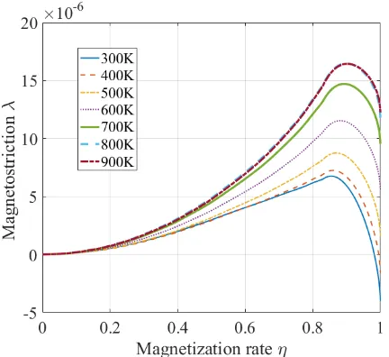
2.3 Magnetostriction curves at different temperatures
It should be noted that the behavior of the magnetostriction curve of polycrystalline iron is related to and . Both of these two parameters change with temperature, and this variation has been measured by other scholars [33], shown in Fig. 5. Both and have
obvious changes with temperature below the Curie temperature (TC). The magnetostriction curves
in the temperature region of 300 K - 900 K are predicted, employing the optimized model, and the
results are shown in Fig. 6. It is important to note that the saturation magnetostriction
of polycrystalline iron increases from approximately at 300 K to at 800
K. In addition, from 300 K to 500 K, the magnetostriction coefficient increases to a positive
maximum value between before decreasing to a negative value, as the magnetic
field strength increases where . The magnetostriction coefficients consistently maintain a
positive value at temperatures between 500 K to 900 K for all values of applied field from
. The result is very significant for studying the excitation efficiency of EMATs via the magnetostrictive mechanism. With an increase of temperature, the magnetic permeability and
electrical conductivity of iron decreases sharply [28, 29], so that the contribution to ultrasonic generation by the Lorentz force mechanism decreases [17, 18]. However, the increase of the
magnetostriction coefficient means that the contribution to ultrasonic generation by the
magnetostriction mechanism may increase with the increasing temperature.In the next section, a
finite element method is applied to simulate the ultrasonic wave generated by the magnetostriction
Fig. 5. The curves of and varying with temperature.
Fig. 6. The magnetostriction curves of polycrystal iron in the temperature region of 300 K to 900 K.
3. Simulations
A 2-D FE model is built using the multi-physics simulation software COMSOL Multiphysics 5.3® to simulate the excitation process of the EMAT, based on the magnetostrictive and Lorentz mechanisms. The physics involved in the coupling process includes electric and magnetic fields
and the resulting force distribution. The coupling between the electric and magnetic fields is based on the classical Maxwell equations, and that between the magnetic field and resultant force is
based on magnetostriction theory, which is the focus of this paper. A nonlinear magnetisation model is adopted to make the simulation more consistent with the actual magnetisation. The iron’s magnetisation curves at different temperatures could be obtained experimentally [34], but are not
readily available, so the Langevin function is used to approximate these curves [35, 36]. Ignoring the hysteresis effect, the material’s magnetisation can be expressed as follows:
[image:9.595.195.411.278.476.2]
where, is the initial susceptibility and is the saturation magnetisation. Both these two parameters are temperature dependent. It is known that as temperature increases from absolute
zero, approaching TC, that the ferromagnetic material’s spontaneous magnetisation gradually
decreases to effectively zero at TC, after which it remains at effectively zero as the sample
becomes paramagnetic [29]. This process can be described by the Ising model, which assumes that the atomic spin direction of the magnetic material obeys the Boltzmann distribution [29, 37], resulting in the spontaneous magnetisation curve with temperature for iron as shown in Fig. 7. In a
ferromagnetic material, the spontaneous magnetisation is the magnetisation of a magnetic domain, which is also amount to saturation magnetisation for polycrystalline when the defects and
impurities are ignored. At the temperature of about 0 K, iron’s spontaneous magnetisation
[38], and the initial magnetic susceptibility . Then, both the initial susceptibility and saturation magnetisation at different temperatures can be got from the Fig. 7.
[image:10.595.194.411.366.548.2]
Fig. 7. Iron’s spontaneous magnetisation curve with temperature. The ordinate has the normalized unit.
The coupling of the magnetic field to the force distribution is more complicated. For
polycrystalline iron, in the absence of stress, the magnetostriciton is assumed to be isotropic [31]. The magnetostriction curves show that for polycrystalline iron, the relationship between magnetic field and stress is highly nonlinear, so a non-linear isotropic magnetostriction model is used in the
simulation. The tensor matrix of strain can be obtained from magnetisation in terms of the
magnetostriction curves. For the magnetisation vector ,
Magnetostrictive strain is a constant volume strain[31], which can be expressed as:
where, the function comes from the magnetostriction curve, and is the deviatoric
tensor of , whose components are defined as follows:
Then, the stress tensor can be expressed as:
where, is the elastic strain tensor, and is the stiffness matrix whose components can be
represented in terms of Young's modulus and Poisson's ratio, which are also temperature
dependent.
Air
Coils
c = 20
Specimen Detection point L if t-of
f = 10
T
= 4
W = 330 Coupling domain
D = 230
b =
35
a = 25
Fig. 8. The geometry of the 2-D FE model used to simulate ultrasonic generation by
magnetostriction. Sample thickness is 4 mm, and width is 330 mm. The coil is a 5 turn, spiral pancake coil, with a lift-off of 10 mm, and the diameter of each turn is 0.68 mm, so the width of
the coil is . Only the coupling domain region is used in the calculation of
[image:12.595.190.391.178.348.2]the magnetostriction coupling to speed up the calculation. All dimensions shown are in millimetres.
[image:12.595.83.506.415.529.2]Fig. 9. The pulse current through the excitation coil, which is sampled from the EMAT transmitter by measuring the voltage across a 0.1 Ω resistor in series with the inductive EMAT coil.
Table 1. Sample’s parameters that employed in the simulation.
Temperature (K) 300 400 500 600 700 800 900
Electrical
Conductivity (MS/m) 5.748 4.252 3.187 2.442 1.913 1.531 1.249
Young's modulus
(GPa) 212.1 208.3 202.3 194.1 183.9 171.5 157.0
Poisson's ratio 0.289 0.294 0.298 0.302 0.306 0.309 0.312
Density (kg/m3) 7858 7829 7797 7763 7727 7689 7652
The geometry of the 2-D FE model used to simulate ultrasonic generation by magnetostriction is shown in Fig. 8, which includes the coil, air, and sample. The coil is copper
wire of diameter 0.68 mm. In principle, the return path of the coil should be added in the model for facticity, as shown in Fig. 12, however, since the return path is relatively far from the surface of the specimen (25 mm), it’s influence is neglected in order to simplify the model. The permeability of air is defined as 1 and conductivity is (this small value provides numerical computation stability). The 1020 steel alloy is defined as the material of the sample, whose conductivity is given by the inbuilt temperature-conductivity curve of COMSOL. Similarly, Young's modulus, Poisson's ratio, and density are also obtained from COMSOL's inbuilt library as
shown in Table 1. To speed up the computation, the magnetostriction coupling is only applied to the part of the sample immediately below the coil, defined as the coupling domain in Fig 8. The
K, in steps of 100 K. A detection point is set on the upper surface of the sample at 230 mm from
the right side of the coil, and its horizontal displacement is recorded as time progresses. The curves of the horizontal displacement of the detection point at 300 K, 500 K, 700 K, 900 K are
shown in Fig. 10. Lamb waves are usually generated in the plate sample, and the simulated S0 Lamb wave is the first wave to reach the detection point, followed by the A0 Lamb wave[26], as shown in the Fig. 10.
[image:13.595.182.426.179.406.2]S0 Lamb waves
Fig. 10. The horizontal displacement of the detection point at different temperature.
The simulation results show that the amplitude of the S0 Lamb wave increases with
temperature in the range of 300 K to 900 K, which support the argument that the contribution of the magnetostriction mechanism to the EMAT’s ultrasound generation increases over a wide temperature range, below TC.
To this point, the electromagnetic excitation and the ultrasonic propagation processes are simulated. In order to facilitate the comparison with experimental results, the EMAT's receiving
process also needs to be taken into account. The function of an EMAT receiver is to convert the vibration of the sample's surface into a voltage signal. For a traditional EMAT receiver, Faraday's law of electromagnetic induction is considered to be the main contributor to this transduction
process [39], although it also includes the magnetoelastic effect [26]. The magnitude of the
voltage signal is proportional to the eddy current density below the probe, which is defined
by the following formula [39]:
where, is the conductivity of the sample, is the particle vibration velocity at the sample's
surface, and is the magnetic flux density. The formula shows that the size of is
proportional to , while, the size of is proportional to the particle displacement and frequency
of vibration. However, both and are variable with temperature. The change of is shown
where, is the magnetic field strength and is the magnetisation. In order to study the relationship between the and temperature, a steady-state nonlinear finite element model (not shown) is established. A permanent magnet NdFeB is employed to provide the static magnetic
field, and the lift-off is set to 1 mm. The configuration is same with the practical experiments, and the reduction of the residual magnetic flux density caused by the temperature-rise of the
permanent magnet is not considered in the simulation. The simulation results show that, in the temperature range of 300 K to 900 K, the magnetic flux density in the sample directly under the permanent magnet changes very little, which can be ignored. Therefore, only the effect of
[image:14.595.179.413.290.503.2]temperature on the electrical conductivity is considered here.
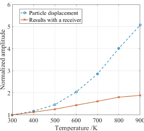
Fig. 11 Normalized amplitude of particle displacement and the amplitude of the received signal varying with the increment of the temperature. The blue broken curve indicates the vibration
amplitude of the particles at the surface. The orange solid curve represents the signal amplitude of the receiving EAMT. These amplitudes are normalized with reference to the value at a temperature
of 300 K.
After considering the effect of temperature on electrical conductivity of the sample, the
growth rate of the signal amplitude is reduced, which is plotted as a curve, as shown in Fig. 11. As a comparison, the change over the temperature of the vibration amplitude of the particles at the surface is also plotted. Both of them increase with a rise in temperature and reach a maximum at
900 K, with an increase of a factor of 5.06 and 1.88 for the particle displacement amplitude and the voltage signal from the EMAT receiver, respectively. In the next section, experiments are
conducted to verify the simulation results.
4. Experiments
configuration of a coil with a bias magnetic field is usually applied in conventional EMATs, whose
mechanisms mainly include Lorentz force and magnetostriction (for magnetic materials). Previous work shows that magnetostriction becomes the main contributor and the Lorentz force could be
ignored when the lift-off of a coil-only transducer is more than 7 mm [26]. The coil-only transducer is employed as the excitation transducer in these experiments with a 10 mm lift-off. The schematic diagram of the experimental configuration is shown in Fig. 12. The excitation coil
is wound on a plastic former. The dimensions of the former in the Y direction and the Z direction are 15 mm and 20 mm respectively. The coil is made of enameled copper wire with a diameter of
0.68 mm, turns 5. A traditional linear coil EMAT with a magnetic field normal to the sample surface is used as the receiving transducer, 462 mm away from the excitation coil as measured from the coil centers. The lift-off of the receiving transducer is 1 mm. A non-conducting layer of
thermal insulation is attached at the bottom of the receiving EMAT to reduce the flow of heat to the EMAT. A 1020 steel alloy plate is used as the sample, with a length L = 620 mm, thickness T =
4 mm, and width 100 mm. The pulse current through the excitation coil is the same as that used in the simulation, as shown in Fig. 9.
S N D=450mm Temperature gun Receiving Coils Magnet Exciting Coils L=620mm Plastic Skeleton Sample
T=4mm Lift off=10mm
Y
X Z
[image:15.595.162.439.312.486.2]O
Fig. 12. Schematic diagram of the experiments configuration.
In the experiments, three 1020 steel plates (0.18% C, 0.25% Si, 0.5% Mn) are tested, and all
the samples are pretreated before the experiments: firstly, the samples are heated and kept at a temperature of 923 K for two hours in an electric resistance furnace, and are then cooled in the furnace to remove most of the stress caused by rolling and cutting, because stress can have a
significant effect on the magnetostrictive parameter[32]. Then, the regions on the surface under the generator and the receiver are polished to remove any oxide layer. A silicone resin paint is
applied to these regions to prevent oxidation at high temperature during the course of the experiments. These samples are tested at these target temperatures: room temperature, 373 K, 473 K, 573 K, 673 K, 773 K, and 873 K. The temperature of the samples drops rapidly when they are
exposed to air, so they are heated above these target temperatures for experimentation. For example, the samples are heated to 500 K when the target temperature is 473 K. An infrared
temperature sensor gun is employed to monitor the surface temperature of the samples. The signals from the receiving transducer are recorded and averaged over 32 times to reduce any electrical noise, and part of the A-scans are shown in Fig. 13. The feature identified on the
estimating the efficiency of the transduction. The waves following the S0 wave are the A0 wave
and the other superpositions of S0 and A0 waves from the edges of the sample.
[image:16.595.136.456.127.439.2]S0 wave
Fig. 13. The recorded waves at the temperature of 298 K, 473 K, 673 K and 873 K. The features in the circles correspond to the S0 model Lamb waves.
Fig. 14. The normalized amplitude of S0 Lamb waves that from the results of the experiments, the
[image:16.595.179.410.521.722.2]permanent magnets and a racetrack coil [17]. The error bars indicate the deviation versus the
average value of the experiment results. Due to the serious electromagnetic interference in our experimental environment, the experimental results still have large errors even after being
averaged.
For each sample, the amplitudes of these S0 waves are calculated first and then are averaged
for all of the samples. The normalized results are shown in Fig. 14. For ease of comparison, both the simulation results and the results from traditional Lorenz based EMAT[17] are also shown in
the Fig. 14. The simulation result is in a good accordance with the experiment result. Both the simulation and the experiment result clearly show that the contribution of magnetostriction mechanism to ultrasonic generation by the EMAT described in the paper, increases as increment of
temperature over the range of 300 K to 900 K. Despite the fact that one would also expect ultrasonic attenuation. Over this increase in temperature one would expect the ultrasonic
attenuation of the sample to increase and the efficiency of the EMAT detector to decrease as the electrical conductivity of the sample falls. The contribution of the Lorenz mechanism to the
generation of ultrasonic waves will also decrease with increasing temperature as again the electrical conductivity of the sample falls. Except for magnetostriction, all other mechanisms involved in the generation and detection of the ultrasonic waves on the sample would cause the
received signal amplitude to fall, clearly demonstrating that there is a significant rise in the contribution of the magnetostrictive measurements in this sample.
5. Discussion
Unfortunately, we have been unable to obtain experimental data on the magnetostriction
curve of polycrystalline iron at high temperatures. It is very difficult to measure the magnetostriction curve of polycrystalline iron at high temperature. The thermal expansion
coefficient of the iron is at the order of / °C, which is an order of magnitude larger than the magnetostriction coefficient ( ), while, it is difficult to keep the temperature constant. So, the static measurement method is not available, only a dynamic measurement method (provide
dynamic magnetic field) could be helpful. Because of the high temperatures, traditional methods of bonding the strain gauges to the sample are unavailable. Besides, iron is easily oxidized when
exposed to air at a high temperature, and the appearance of an oxide layer would either detach or detrimentally affect a strain gauge measurement. Although a method for measuring the magnetostriction of a material at high temperatures is discussed in the published literature [34],
the authors point out that it is not suitable for iron because of surface oxidisation.
In the experiments, the receiving EMAT is isolated from the sample by a piece of
temperature-resistant material with the lift-off of 1 mm, but the receiving EMAT will still be heated, and the efficiency of EMAT will be reduce, primarily due to a slight drop in the permanent magnet's flux density and a decrease in the conductivity of the wire in the EMAT's coil[17]. In the
experiment, the receiver is cooled before the test, and the duration of the single test process is limited to within 5 s in order to reduce the temperature rise of the receiving probe. The receiver’s
maximum temperature reaches about 60 degree Celsius which is still in the work temperature range, so that any effects of decreased signal amplitude due to the detection EMAT heating up are not considered.
residual stress caused by this operation should be discussed. Usually, machining operations such
as milling, planning and broaching significantly cause the residual stress on the surface of the material. Nevertheless, abrasion operations such as polishing, and honing are performed with
lower speed, pressure and hence incorporate fewer residual stresses. In addition, a softer material 1020 steel is acted as the sample which can also reduce the residual stress caused by the polishing operation. Therefore, the affection caused by the polishing operation to current results is not been
[image:18.595.208.401.198.375.2]observed.
Fig. 15 The comparison results between the samples exposed to air and coated with protective paint. the Y-axis data is the normalized amplitude of S0 lamb waves. The error bars
indicate the deviation versus the average value of the experiment results.
Iron and low carbon steels are rapidly oxidized in high temperatures, forming a surface oxide layer. One of its oxides, Fe3O4 (magnetite), is also a highly magnetostrictive magnetic material,
which if present on the sample surface during experiments would prevent validation of the simulation results. Therefore, in the experiment, all the samples are coated with high-temperature paint after heat treating for stress removal and polishing, to prevent the samples from being
oxidized in a high temperature environment. However, in most real high-temperature applications, no anti-oxidation measures are taken on the steel and an oxide layer grows on the surface of the
steel, increasing in thickness with both time and temperature. Because real samples and in some cases experimental measurements are performed when magnetite is present on the sample surface, some additional measurements are taken for this situation. A number of samples are not polished
or painted after being destressed, and they are directly exposed to the ambient atmosphere during heating. The experimental results for these measurements are shown in figure 15. It is clear that
the magnetostrictive effect in the samples with a magnetite oxide layer is more pronounced as the temperature increases. The amplitude of S0 wave rises with temperature in the range of 300 K to 773 K, and then decreases in the temperature range of 773 K to 873 K. This is because as the
temperature approaches closer to magnetite's Curie temperature, it's magnetostriction parameter reduces, until it becomes non-magnetic at its Curie point of 838 K [40]. It is also possible that the
Fig. 16 The magnetisation distribution in the magnetostriction coupling region. The maximum
magnetisation reaches a maximum when the time is 5 . The temperature is set
to 300 K.
A typical EMAT is usually configured with an excitation coil and a bias magnetic field (vertical or horizontal). In order to achieve a higher efficiency, the bias magnetic field strength is generally set
to a large value. The dynamic magnetic field generated by the excitation coil is superimposed on the bias magnetic field, so that the sample is mainly magnetized in the domain rotation phase [6]. However, the generator shown in this paper has a large lift-off distance (10 mm) and without a
bias magnetic field, so the magnetisation in the sample is much smaller. Fig. 16 shows the
distribution of magnetisation when it reaches its maximum value at 5 . The maximum
magnetisation is , while the saturation magnetisation is at 300
[image:19.595.190.405.74.227.2]K. So, the maximum magnetisation ratio is about 0.4, which is still in the domain wall movement phase. Defects and impurities in the crystal structure usually form potential energy barriers to domain wall movement, which leads to energy loss. However, the numerical simulation doesn’t consider this loss. So, the result of the simulation may overestimation the transduction efficiency.
Fig. 6 shows that, as the temperature rises, the slope of the magnetostriction curve increases at the domain wall movement phase, which is seemly inverse in the domain rotation phase. So, a different conclusion may be got in a traditional EMAT, which needs further research and is beyond
the scope of this paper.
This paper shows that for the generation EMAT described in this paper, the contribution of
the magnetostrictive mechanism to the energy conversion efficiency of electrical to ultrasonic rises with increasing temperature, while the contribution of the Lorentz force mechanism decreases. Note though it has not been proved that, at high temperature on steel, the Lorentz force
contribution ratio is smaller than that of the magnetostrictive mechanism for a conventional EMAT, and previous work would indicate that for conventional EMATs, the Lorentz force remains the
dominant generation mechanism at increased temperature. Even so, it provides a theoretical basis for the structural design of a type of EMAT that could be applied at high temperatures.
In addition to temperature, the magnetostrictive coefficient of the material are also affected
by the material composition, internal impurities, stress, and other factors, that are not considered in this paper, and will be the subject of further research.
6. Conclusions
Based on Brown’s the magnetic domain wall movement model and Lee’s the domain rotation
magnetostriction curves of polycrystalline iron for temperature range 300 K to 900 K are given,
which reveal that the saturated magnetostriction coefficient changes from to about
.
A 2-D non-linear isotropic magnetostriction FE model is developed to simulate the Lamb waves generated by EMAT’s magnetostriction mechanism in 4 mm steel plate. The simulation results show that the amplitude of S0 Lamb wave rise evidently with the increment of temperature.
Series experiments are employed to verify the simulation. Experiment results verify that the contribution of the magnetostriction mechanism to EMAT’s efficiency increases with increasing
temperature. This conclusion provides an important basis for the optimization of the EMAT probe used in high temperature testing or measurement.
Reference:
[1] Thompson RB, Alers GA, Tennison MA. Application of Direct Electromagnetic Lamb Wave
Generation to Gas Pipeline Inspection. Ultrasonics Symposium. Boston, MA, USA1972. p.
91-4.
[2] Thompson RB. New Electromagnetic Transducer Applications. Proceedings of the
ARPA/AFML Review of Progress in Quantitative NDE. Ithaca, NY, USA1978. p. 340 - 4.
[3] Thompson RB, Elsley RK, Peterson WE, Vasile CF. An EMAT for Detecting Flaws in Steam
Generator Tubes. Ultrasonics Symposium. New Orleans, LA, USA1979. p. 562-7.
[4] Thompson RB, Vasile CF. New EMAT Applications: Ultrasonic Ellipsometer and Detection
of Cracks under Fasteners. Proceedings of the ARPA/AFML Review of Progress in
Quantitative NDE. La Jolla, CA, USA1979. p. 40-5.
[5] Burrows SE, Fan Y, Dixon S. High temperature thickness measurements of stainless steel
and low carbon steel using electromagnetic acoustic transducers. Ndt&E Int. 2014;68:73-7.
[6] Ribichini R, Cegla F, Nagy PB, Cawley P. Quantitative modeling of the transduction of
electromagnetic acoustic transducers operating on ferromagnetic media. IEEE Transactions
on Ultrasonics Ferroelectrics & Frequency Control. 2010;57:2808.
Lamb Waves. IEEE Transactions on Sonics & Ultrasonics. 1973;20:340-6.
[8] Thompson RB. A model for the electromagnetic generation of ultrasonic guided waves in
ferromagnetic metal polycrystals. IEEE Transactions on Sonics & Ultrasonics. 1978;25:7-15.
[9] Thompson RB. New Configurations for the Electromagnetic Generation SH Waves in
Ferromagnetic Materials. Ultrasonics Symposium. Cherry Hill, NJ, USA: IEEE; 1978.
[10] William Fuller Brown J. Domain Theory of Ferromagnetics Under Stress Part II.
Magnetostriction of Polycrystalline Material. Phys Rev. 1938;53:482-91.
[11] Lee EW. Magnetostriction Curves of Polycrystalline Ferromagnetics. Proceedings of the
Physical Society. 1958;72:249-58.
[12] Vasile CF, Thompson RB. Excitation of horizontally polarized shear elastic waves by
electromagnetic transducers with periodic permanent magnets. Journal of Applied Physics.
1979;50:2583-8.
[13] Moran TJ, Panos RM. Electromagnetic generation of electronically steered ultrasonic bulk
waves. Journal of Applied Physics. 1976;47:2225-7.
[14] Zhou JJ, Zheng Y, Liu HB, Zheng H, Li SJ. Non-destructive testing of stainless steel in
high temperature using electromagnetic acoustic transducer. Materials Research Innovations.
2015;19:S10-291-S10-4.
[15] Urayama R, Uchimoto T, Takagi T. Application of EMAT/EC Dual Probe to Monitoring of
Wall Thinning in High Temperature Environment. Ceskoslovenska Otolaryngologie.
2009;33:1317-27.
[16] Kogia M. Electromagnetic Acoustic Transducers Applied to High Temperature Plates for
[17] Kogia M, Gan TH, Balachandran W, Livadas M, Kappatos V, Szabo I, et al. High
Temperature Shear Horizontal Electromagnetic Acoustic Transducer for Guided Wave
Inspection. Sensors. 2016;16:582.
[18] Hernandez-Valle F, Dixon S. Initial tests for designing a high temperature EMAT with
pulsed electromagnet. Ndt&E Int. 2010;43:171-5.
[19] Dhayalan R, Murthy VSN, Krishnamurthy CV, Balasubramaniam K. Improving the signal
amplitude of meandering coil EMATs by using ribbon soft magnetic flux concentrators (MFC).
Ultrasonics. 2011;51:675-82.
[20] Kang L, Zhang C, Dixon S, Zhao H, Hill S, Liu MH. Enhancement of ultrasonic signal using
a new design of Rayleigh-wave electromagnetic acoustic transducer. Ndt&E Int.
2017;86:36-43.
[21] Pei CX, Zhao SQ, Xiao P, Chen ZM. A modified meander-line-coil EMAT design for signal
amplitude enhancement. Sensor Actuat a-Phys. 2016;247:539-46.
[22] Gaerttner MR, Wallace WD, Maxfield BW. Experiments Relating to the Theory of
Magnetic Direct Generation of Ultrasound in Metals. Physical Review. 1969;184:702-4.
[23] Fortunko CM, Thompson RB. Optimization of Electromagnetic Transducer Parameters for
Maximum Dynamic Range. Ultrasonics Symposium. Annapolis, MD, USA1976. p. 12-6.
[24] Ribichini R, Cegla F, Nagy PB, Cawley P. Experimental and numerical evaluation of
electromagnetic acoustic transducer performance on steel materials. Ndt&E Int. 2012;45:32-8.
[25] Ribichini R, Nagy PB, Ogi H. The impact of magnetostriction on the transduction of normal
bias field EMATs. Ndt&E Int. 2012;51:8-15.
Generating and Receiving S0 Lamb Waves in Ferromagnetic Steel Plate. Sensors.
2017;17:1023.
[27] Aoyanagi M, Wakatsuki N, Mizutani K, Ebihara T. Design of piezoelectric probe for
measurement of longitudinal and shear components of elastic wave. Japanese Journal of
Applied Physics. 2017;56:07JD14.
[28] Taylor GR, Isin A, Coleman RV. Resistivity of Iron as a Function of Temperature and
Magnetization. Physical Review. 1968;165:621-31.
[29] Jiles, David C. Introduction to Magnetism and Magnetic Materials: Chapman and Hall;
1998.
[30] Wang WY, Liu B, Kodur V. Effect of Temperature on Strength and Elastic Modulus of
High-Strength Steel. Journal of Materials in Civil Engineering. 2013;25:174-82.
[31] Lee EW. Magnetostriction and Magnetomechanical Effects: s.n.; 1955.
[32] Yamasaki T, Yamamoto S, Hirao M. Effect of applied stresses on magnetostriction of low
carbon steel. Ndt&E Int. 1996;29:263-8.
[33] Callen HB, Callen ER. Theory of High-Temperature Magnetostriction. Physical Review.
1963;132:991-6.
[34] Lorenz BE, Jr CDG. Apparatus for high temperature magnetostriction measurement of
bulk samples. Review of Scientific Instruments. 2004;75:2770-2.
[35] D’Yachenko SV, Zhernovoi AI. The Langevin formula for describing the magnetization
curve of a magnetic liquid. Technical Physics. 2016;61:1835-7.
[36] Harrison RG. Calculating the spontaneous magnetization and defining the Curie
[37] Yang CN. The Spontaneous Magnetization of a Two-Dimensional Ising Model. Physical
Review. 1952;85:808-16.
[38] Danan H, Herr A, Meyer AJP. New Determinations of the Saturation Magnetization of
Nickel and Iron. Journal of Applied Physics. 1968;39:669-70.
[39] Jian X, Dixon S, Quirk K, Grattan KTV. Electromagnetic acoustic transducers for in- and
out-of plane ultrasonic wave detection. Sensors & Actuators A Physical. 2008;148:51-6.
[40] Levy D, Giustetto R, Hoser A. Structure of magnetite (Fe 3 O 4 ) above the Curie

![Fig. 4. The prediction results of optimized model for polycrystalline iron’s magnetostriction curves (Room temperature), and the Yamasaki’s measurement results [32]](https://thumb-us.123doks.com/thumbv2/123dok_us/9425614.446618/8.595.182.401.106.304/prediction-results-optimized-polycrystalline-magnetostriction-temperature-yamasaki-measurement.webp)