warwick.ac.uk/lib-publications
Original citation:Taylor, Celia A.. (2017) Li, Rui, Leng, Chenlei and You, Jinhong. (2017) A semiparametric regression model for longitudinal data with non-stationary errors. Scandinavian Journal of Statistics .
Permanent WRAP URL:
http://wrap.warwick.ac.uk/91429
Copyright and reuse:
The Warwick Research Archive Portal (WRAP) makes this work by researchers of the University of Warwick available open access under the following conditions. Copyright © and all moral rights to the version of the paper presented here belong to the individual author(s) and/or other copyright owners. To the extent reasonable and practicable the material made available in WRAP has been checked for eligibility before being made available.
Copies of full items can be used for personal research or study, educational, or not-for-profit purposes without prior permission or charge. Provided that the authors, title and full
bibliographic details are credited, a hyperlink and/or URL is given for the original metadata page and the content is not changed in any way.
Publisher’s statement:
"This is the peer reviewed version of the following article Li, Rui, Leng, Chenlei and You, Jinhong. (2017) A semiparametric regression model for longitudinal data with non-stationary errors. Scandinavian Journal of Statistics . doi:10.1111/sjos.12284 has been published in final form athttp://dx.doi.org/10.1111/sjos.12284
This article may be used for non-commercial purposes in accordance with Wiley Terms and Conditions for SelfArchiving."
A note on versions:
The version presented here may differ from the published version or, version of record, if you wish to cite this item you are advised to consult the publisher’s version. Please see the ‘permanent WRAP URL’ above for details on accessing the published version and note that access may require a subscription.
Data with Non-stationary Errors
RUI LI
School of Statistics and Information, Shanghai University of International Business and Economics
CHENLEI LENG
Department of Statistics, University of Warwick
JINHONG YOU
Key Laboratory of Mathematical Economics (SUFE), Ministry of Education of China School of Statistics and Management, Shanghai University of Finance and Economics
Abstract Motivated by the need to analyze the National Longitudinal Surveys (NLS) data,
we propose a new semiparametric longitudinal mean-covariance model in which the effects on dependent variable of some explanatory variables are linear and others are nonlinear, while the
within-subject correlations are modeled by a non-stationary autoregressive error structure. We develop an estimation machinery based on least squares technique by approximating nonparametric
functions via B-spline expansions, and establish the asymptotic normality of parametric estimators as well as the rate of convergence for the nonparametric estimators. We further advocate a new
model selection strategy in the varying-coefficient model framework, for distinguishing whether a component is significant and subsequently whether it is linear or nonlinear. Besides, the proposed
method can also be employed for identifying the true order of lagged terms consistently. Monte Carlo studies are conducted to examine the finite sample performance of our approach and an
application of real data is also illustrated.
Key words: autoregressive process; B-splines; model selection; rate of convergence; SCAD
penalty.
Running Head. Semiparametric longitudinal data model
1
Introduction
Longitudinal observations are repeated measurements from the same subject over time and
of the most distinguishing characteristics. Informative identification of this correlation
structure has gained considerable attention in recent years since the pioneering work of Liang
& Zeger (1986), and many approaches have already been developed. Diggle et al. (2013)
provided a comprehensive review on the modeling and inference of longitudinal analysis.
The National Longitudinal Surveys (NLS) are a set of surveys designed for gathering
information at multiple points in time on the labor market activities and other significant
events of several groups of men and women. In this paper, we focus on the analysis of a
NLS subset named nlswork.dta in which 1357 annual observations were obtained from 266
subjects graduated from college during 1970 and 1988. The number of observations per
subject ranges from 4 to 11, which shows that this data set is irregular and possibly has
subject-specific observation time. Specifically, what factors have effects on the average level
of one’s salary and how do the significant ones work are the two issues we are most interested
in. Therefore one’s wage in this longitudinal data set is regarded as dependent variable and
the logarithm of wage (lwage) is taken for deriving measurements. The possible correlated
explanatory variables include interviewed year (year), usual hours worked (hours), one’s age
in current year (age), total work experience (exper), weeks worked last year (wks.work),
job tenure years (tenure) and current grade completed (educ). Then both the significance
of correlation between these variables andlwage, and the linear/nonliear effects on lwageof
the significant ones are expected to be identified practically.
Motivated by the analysis of this NLS data set, we propose a semiparametric model
naively since both scatter diagrams and Pearson correlation tests indicate that exper and
tenure have nonlinear effects onlwage while other variables have linear effects. In addition,
we only put age, one’s age in current year, into the model for circumventing the possible
multi-collinearity between the variables age and year. Specifically the model considered is
lwagei,j = hoursi,jβ1+agei,jβ2+educi,jβ3 +wks.worki,jβ4
+α1(experi,j) +α2(tenurei,j) +εi,j, (1)
where βk, k = 1, . . . ,4 are coefficient parameters and αl(·), l = 1,2 are unknown smooth
functions, while εi,j is random error with mean 0 and allowed to be heteroscedastic.
been developed like series estimation (e.g. Li, 2000), kernel smoothing (e.g., Fan & Li,
2003) and regression spline (e.g. Liu et al., 2011). As the first attempt to analyze this
data set, we suppose the disturb term εi,j to be white noise, and estimate the parametric
and nonparametric components simultaneously based on spline approximation and least
squares technique. Naturally, the fitting residualεbi,jcan be easily obtained from the resulting
consistent estimators (Liang & Zeger, 1986). A closer look at the scatter diagrams of εbi,j
shows a clear trend, which motivates us to get a more efficient estimator by exploring the
possible correlation structure among the fitting residual εbi,j.
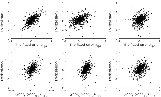
[Figure 1 about here.]
Graphical comparisons of εbi,j in Figure 1 show an obvious dependence of εbi,j on its
predecessors bεi,j−1,bεi,j−2 and bεi,j−3 in the top three panels. In the typical longitudinal
studies, subjects may be commonly observed at irregular time intervals. Then it is natural
to assess whether this dependence between two error components also varies with their
time distance. Towards this end, we further plot the jth (j > 3) fitting residual against
time-distance dependent residuals (yeari,j −yeari,j−1)εbi,j−1, (yeari,j −yeari,j−2)εbi,j−2 and
(yeari,j−yeari,j−3)εbi,j−3 respectively in the bottom three panels. We can easily observe that
the correlations showed in the far left two panels are relatively strong, and this correlation
gradually decreases as the time distance between two measurements increases.
The discussions above motivate a more general semiparametric model as the follows:
Yi,j = X⊤i,jβ+α1(Ui,j,1) +· · ·+αq(Ui,j,q) +εi,j,
εi,j =
s
∑
r=1
(ar+br∆ti,j,r)εi,j−r+ei,j with ∆ti,j,r =ti,j−ti,j−r, (2)
where i= 1, . . . , nand j =s+ 1, . . . , mi, and the total sample size is N =
∑n
i=1mi. Model
(2) allows more nonparametric covariates to be included than the partially linear structure of
Lenget al.(2010), and employs a non-stationary and time-adaptive autoregressive process for
identifying the within-subject correlation of repeated measurements. We useYi,jfor denoting
the jth measurement of the ith subject, Xi,j = (1, Xi,j,1, . . . , Xi,j,p)⊤ and Ui,j,l, l = 1, . . . , q
are strictly exogenous regressors on which the unknown smooth functions {αl(Ul)}
q
l=1 are
(β1, . . . , βp)⊤ and the autoregressive coefficients are a= (a1, . . . , as)⊤ and b = (b1, . . . , bs)⊤
respectively, whileei,j’s are i.i.d. random disturbs with mean zero and varianceσe2. A similar
autoregressive error structure presented in equation (2) was proposed by Bai et al. (2015)
for partially linear model. Obviously, the partially linear additive model is more flexible and
useful than partially linear model because the former allows several nonparametric terms
for some regressors. Thus, it is possible to explore more complex and accurate relationships
between the response and explanatory variables.
Recent years have seen growing interests in developing flexible mean and covariance
models for analyzing longitudinal data. The semiparametric mean model in (2) was widely
studied, see e.g., Lin & Ying (2001), Lin & Carroll (2001a, 2001b), He et al. (2002), Wang
(2003), He et al. (2005), Wang et al. (2005), Lian et al. (2014) and Cheng et al. (2014).
There was also a large literature for developing new models for characterizing the covariance
structure, see for example, Pourahmadi (1999), Fanet al.(2007), Wu & Pourahmadi (2003),
Fan & Li (2004), Fan & Wu (2008), Leng et al. (2010), Li (2011), Zhang & Leng (2012),
Zhou & Qu (2012). A recent line of research for variable selection has also undergone rapid
development, see e.g., Fan & Li (2001), Wang et al. (2009), Liu et al. (2011), Ma et al.
(2013). Among these studies, a working correlation model for the variance is often assumed.
Additionally, Zhanget al. (2011) proposed a method for distinguishing linear and nonlinear
variables for cross sectional data model in the framework of reproducing kernel Hilbert spaces.
In contrast, our treatment is for repeat measurement that is very common in practice and
model the dependence explicitly motivated by the analysis of NLS data. We make use of basis
expansion approach via B-splines that is much simpler. Our model selection method is also
distinctively different, and provides an alternative view for identifying linear and nonlinear
variables by transforming one general model into varying-coefficient structure. In addition,
the proposed model selection method could be used to determine the order of time lag and
time distance variables in modeling εi,j as well. This is also important due to the fact that
misspecification of the error structure will resultant in inefficient estimation and uncorrect
statistical inference. It should also be noted that the non-stationary error structure in (2) is
essentially different from that of Lenget al.(2010). Specifically, the number of autoregressive
coefficient in Lenget al.(2010), generated from Cholesky decomposition of covariance matrix,
error structure is finite and usually small, no matter how large T is. So, our method could
be used to model the functional data sets as well, however, the method of Leng et al.(2010)
does not work for the the functional data sets.
The layout of the remainder is as follows. In Section 2, we construct an efficient
semiparametric least squares estimator for both the parametric and nonparametric
components when model structure is completely known. Besides asymptotic property is also
established accordingly. In Section 3 we propose a novel shrinking method for identifying
the structure of true model, and further show that the resulting penalized estimators have
the same asymptotic properties as if the true submodel was known in advance. Numerical
studies from Monte Carlo procedure and a real data analysis are also illustrated in Section 4.
Section 5 presents summary remarks. All the technical details are relegated to the Appendix.
2
Semiparametric least squares estimation
Polynomial spline is commonly employed for approximating smooth function for its stability
in computations. As pointed by de Boor (1978) and Schumaker (1981), spline function is
actually piecewise polynomial smoothly connected at a series of knots. In specific, suppose
u=u0 < u1 < . . . < uκn < uκn+1 = ¯u
be a knot sequence, a spline functions(u) of degreed >1 (orderd+1) is a function satisfying
that s(u) belongs to Cd−1[u,u¯] and its restriction to each [uk−1, uk) for k = 1, . . . , κn and
[uκn, uκn+1] is a polynomial of degree at most d. We use S
d
κn(u) to denote the spline space
spanned by a group of spline basis {Bk(u)}Kk=1, which implies that there exists real vector
(θ1, . . . , θK) such that s(u) =
∑K
k=1Bk(u)θk where K =Kn=κn+d is allowed to approach
to infinity asn increases.
Following the discussion above, each αl(Ul) can be approximated by a spline function
sl(Ul) = ∑Kl
k=1Bl,k(Ul)θl,k with Kl =κl+d, 1 ≤l ≤q. Subsequently the mean structure of
model (2) can be expressed as
Yi,j =X⊤i,jβ+
q
∑
l=1
{ K
l
∑
k=1
Bl,k(Ui,j,l)θl,k
}
where ε∗i,j = ∑ql=1{∑Kl
k=1Bl,k(Ui,j,l)θl,k−αl(Ui,j)
}
+ εi,j. The use of Lemma 1 in the
Appendix implies that ε∗i,j = εi,j +op(1). As a result, same as Cochrane & Orcutt (1949),
MaCurdy (1982) and Wang et al.(2007) one can estimate (β,θ1, . . . ,θq,a,b) by minimizing
n
∑
i=1
mi
∑
j=s+1
Yi,j −
s
∑
r=1
(ar+br∆ti,j,r)Yi,j−r−
{
Xi,j− s
∑
r=1
(ar+br∆ti,j,r)Xi,j−r
}⊤ β − q ∑ l=1 Kl ∑ k=1 {
Bl,k(Ui,j,l)−
s
∑
r=1
(ar+br∆ti,j,r)Bl,k(Ui,j−r,l)
}
θl,k
]2
def
= L0(β,θ,a,b). (3)
According to Cochrane & Orcutt (1949), when a normal distribution is assumed for the
errors εi,j, the resultant estimator of the parameters in (3) is also the maximum likelihood
estimator.
Noting the interaction of unknown parameters in (3), an iterative estimating process is
expected from an appropriate initial estimator. In addition, the objective function defined
in (3) makes no use of {Yi,j,Xi,j, ti,j : i = 1, . . . , n; j = 1, . . . , s} and perhaps results in
the efficiency loss of estimation. This motivates the following objective function using full
observations:
LN(β,θ,a,b) = L0(β,θ,a,b) +
n ∑ i=1 s ∑ j=1 {
Yi,j−X⊤i,jβ−
q ∑ l=1 Kl ∑ k=1
Bl,k(Ui,j,l)θl,k
}2
.
Then the updated LSE are
(βbN,bθN,baN,bbN) = argminLN(β,θ,a,b), (4)
and the estimator of αl(Ul) follows as αbl,N(Ul) =
∑Kl
k=1Bl,k(Ul)θbl,k,N, l= 1, . . . , q.
Suppose X be generated by the function vector η(u) = (η1(u), . . . , ηp(u))⊤ =
(∑ql=1η1,l(ul), . . . ,
∑q
l=1ηp,l(ul))⊤ as Xi,j = η(Ui,j) +δi,j for i = 1, . . . , n, j = 1, . . . , mi,
where δi,j = (δi,j,1, . . . , δi,j,p)⊤ is random disturb term satisfying E(δi.j|Ui,j) = 0.
For ease of notation, we write δ∗i,j = δi,j −
∑s
r=1(ar + br∆ti,j,r)δi,j−r and ζi,j =
matrices Γ and Λ, 1 n n ∑ i=1 ( s ∑ j=1
δi,jδ⊤i,j +
mi
∑
j=s+1
δ∗i,jδ∗⊤i,j )
P
→Γ and 1
n n ∑ i=1 mi ∑
j=s+1
ζi,jζ⊤i,j →P Λ.
The asymptotic property in the text followed is established asN (or n) tends to infinity.
Theorem 1. Suppose that assumptions A1−A6 in the Appendix are satisfied, then
(i) √n(βbN −β)→D N(0,Γ−1ΣΓ−1), where
1 n n ∑ i=1 [
σ2e
mi
∑
j=s+1
δ∗i,jδ∗⊤i,j + (δi,1, . . . ,δi,s)cov{(εi,1, . . . , εi,s)⊤}(δi,1, . . . ,δi,s)⊤
]
P
→Σ;
(ii) √n{(ba⊤N,bb⊤N)⊤−(a⊤,b⊤)⊤}→DN(0, σ2
eΛ−
1);
(iii) max1≤l≤q∥αbl,N−αl∥2L2 =Op
(
maxlKl/N+ maxlKl−4
)
, where ∥α∥L2 = (
∫
uα
2(u)du)1/2.
The asymptotic normality of parametric estimators can serve as a basis for further
inference, while the asymptotic covariance matrices for βbN and (baN,bbN) have a relatively
simple and explicit structure that enables us to construct the estimator of variance
straightforwardly without resorting to resampling-based methods. However these implements
involve the estimation of σ2
e,Γ,Σ, and Λ. Actually we can estimate σ2e by
b
σ2e,N = 1
n n
∑
i=1
1
mi−s
mi
∑
j=s+1
{ b
εi,j−
s
∑
r=1
(bar,N +bbr,N∆ti,j,r)bεi,j−r
}2
,
where bεi,j =Yi,j −X⊤i,jβbN −αb1,N(Ui,j,1)− · · · −αbq,N(Ui,j,q).
For simplicity of expression, we write Bl(Ui,j,l) = (Bl,1(Ui,j,l), . . . , Bl,Kl(Ui,j,l))⊤, Bl =
(Bl(U1,1,l), . . . ,Bl(Un,mn,l))⊤andPBl =Bl(B
⊤
l Bl)−1B⊤l , similarlyPB =B(B⊤B)−1B⊤with
B= (B1, . . . ,Bq). Define ˜X = (I−PB)X. Write ˜X∗i,j = ˜Xi,j−
∑s
r=1(bar,N+bbr,N∆ti,j,r) ˜Xi,j−r
and ζbi,j = (bεi,j−1, . . . ,εbi,j−s,εbi,j−1∆ti,j,1, . . . ,εbi,j−s∆ti,j,s)⊤ for i= 1, . . . , n, j =s+ 1, . . . , mi.
Then we can estimate Γ,Λ and Σ respectively by
b
ΓN = 1 N
n
∑
i=1
(∑q
j=1
˜
Xi,jX˜⊤i,j +
mi
∑
j=q+1
˜
X∗i,jX˜∗⊤i,j
)
b
ΛN = 1
N−nq
n
∑
i=1
mi
∑
j=q+1
b
ζi,jbζ⊤i,j and
b
ΣN = 1 N
n
∑
i=1
[ b
σe,N2
mi
∑
j=q+1
˜
X∗i,jX˜∗⊤i,j +
(∑q
j=1
˜
Xi,jεbi,j
)(∑q
j=1
˜
Xi,jbεi,j
)⊤]
.
Theorem 2. Suppose that the conditions in Theorem 1 are satisfied. Then we have that
√
N −sn(bσe,N2 −σe2)→D N(0,var(e2i,j)),
b
ΓN
P
→Γ, ΛbN
P
→Λ, and ΣbN
P
→Σ.
The asymptotic results in Theorem 2 lead to consistent estimators of the asymptotic
covariance matrices of βbN and (baN⊤,bb⊤N)⊤.
3
Model identification
We have derived the consistent estimates for both parametric and nonparametric components
when the model structure in (2) is completely known. However, it’s commonly a different
story in practice since we have no prior knowledge on the significance of these variables
nor the forms of their effects on the response variable. Therefore we propose a method in
this section for identifying the significant variables and further distinguish the corresponding
effects of linearity with nonlinearity on the responses.
Specifically, we employ an initial nonparametric additive model below,
Yi,j =µ+G1(Zi,j,1) +· · ·+GL(Zi,j,L) +εi,j (5)
where the regressorZ is perhapsX and U defined in model (2), andGl(Zl), l= 1, . . . , L are
unknown smooth functions satisfying E(Gl(Zl)) = 0, while εi,j ia also similarly defined as
that in model (2). Then we expect to identify the significance and linear/nonlinear effects
of Z on Y. For ease of implementation, we rewrite the model (5) as the following varying
coefficient framework,
with g(z) =G(z)/z. Since the point set {0} is zero-measure for some compact support, we
can assume that z ̸= 0 here without loss of generality. The varying coefficient model in (6)
is actually a transformation of the additive model (5), which is used just for facilitating the
identification of possible linear effect of covariate on response variable only. That means
the variable Zl is linearly correlated with the response once gl(Zl)≡ constant in the model
(6), and then the model (5) can be identified as the semiparametric model in (2). Following
the discussions in Section 2, there is θ∗l = (θ∗l,1, . . . , θ∗l,K
l)
⊤ and basis functions B∗
l(Z) =
(Bl,∗1(Z), . . . , Bl,K∗
l(Z))
⊤ such that
gl(Zi,j,l) =
Kl
∑
k=1
Bl,k∗ (Zi,j,l)θ∗l,k+op(1), l = 1, . . . , L.
We can immediately conclude that (i) Gl(zl) ≡ 0 is equivalent to gl(zl) ≡0 and ||θ∗l|| = 0;
(ii) Gl(zl) is linear function if gl(zl)≡constant̸= 0, which is equal to ||θ∗l|| ̸= 0 and
||θ∗l||2d def= θ∗⊤l DKl×Klθ ∗
l =θ∗⊤l
1 −1 0 . . . 0
−1 2 1 . . . 0
..
. ... ... ... ...
0 . . . −1 2 −1
0 . . . 0 −1 1
θ∗l = 0. (7)
We centralize the observation Yi,j first for removing the intercept term µ from (6) and
write the unknown index set of zero, constant and function of regressors as S0,Sc and Sv
respectively. Then we identify these sets by adding penalization to the following quadratic
loss function:
˜
L0(θ∗,a,b) =
n
∑
i=1
mi
∑
j=s+1
[
Yi,j−
s
∑
r=1
(ar+br∆ti,j,r)Yi,j−r−
L ∑ l=1 Kl ∑ k=1 {
Zi,j,lBl,k∗ (Zi,j,l)−
s
∑
r=1
(ar+br∆ti,j,r)Zi,j−r,lBl,k∗ (Zi,j−r,l)
}
θ∗l,k
]2 + n ∑ i=1 s ∑ j=1 {
Yi,j−
L ∑ l=1 Kl ∑ k=1
Zi,j,lBl,k∗ (Zi,j,l)θl,k∗
}2
Then the penalized least squares estimator (˘θ∗N,a˘N,b˘N) can be constructed by minimizing
˜
Lp
N(θ∗,a,b) = L˜0(θ∗,a,b) +N
s
∑
r=1
pλ1(||ξr||) +N
L
∑
l=1
pλ2(||θ
∗
l||)
+N
L
∑
l=1
pλ3(||θ
∗
l||d)I(||θ∗l|| ̸= 0), (9)
where θ∗⊤ = (θ∗⊤1 , . . . ,θ∗⊤L ), ξr⊤ = (ar, br) and pλ(·) is the smoothly clipped absolute
deviation (SCAD) penalty defined in Fan & Li (2001). Actually the first derivative of SCAD
is used in implementation,
p′λ(·) = λ
{
I(| · |< λ) + (aλ− | · |)+
(a−1)λ I(| · |< λ)
}
sgn(·)
with λ > 0 be tuning parameter and a= 3.7 from a Bayesian point of view. The penalized
estimator of nonprarametric function follows as ˘Gl,N(Zi,j,l) = {B∗⊤l (Zi,j,l)˘θ
∗
l,N}Zi,j,l.
Since the difficulty raised by indicatorI(·) in (9), we employ an iterative process for an
alternative approach in terms of computational simplicity. At the first stage, we distinguish
zero coefficients from the non-zero ones by minimizing
Lp
1(θ∗,a,b) = ˜L0(θ∗,a,b) +N
s
∑
r=1
pλ1(||ξr||) +N
L
∑
l=1
pλ2(||θ
∗
l||). (10)
Let ˘S0 be the estimated set of S0, and ˘θN∗,a˘N,b˘N be the nonzero estimates in this stage.
Based on these estimates, we minimize
Lp
2(θ∗,˘aN,b˘N) = ˜L0(θ∗,˘aN,b˘N) +N
L
∑
l=1
pλ3(||θ
∗
l||d)I(||θ˘
∗
l,N|| ̸= 0) (11)
for identify the constant and varying coefficients over the complement of ˘S0. Let ˘Sc and
˘
Sv be estimated index sets of Sc and Sv respectively. Then, repeating (10) and (11) above
until the solution converges and denoting the final estimator as (˘θ∗N,˘aN,b˘N) for avoiding
the abuse of notation.
Another key problem in the implementation is the choice of tuning parameters λ1, λ2
et al. (2008) and Wang et al. (2009). We use the Bayesian information criterion (BIC) for
its finite sample performances (see, e.g. Wang et al., 2007) and select these parameters by
minimizing
BIC(λ) = ln
{
1
NL˜
p
N(θ∗,a,b)
}
+dfln(N)
N , (12)
where df is the degree of freedom of the model.
Suppose (a0,b0) be the true value of (a,b) and (a01,b01) be thes0nonzero entries, while
G0 = (G⊤0c,G⊤0v,0⊤)⊤ witb G0c = (G01, . . . , G0L′
0)
⊤ and G
0v = (G0L′
0+1, . . . , G0L0)
⊤ be the
constant and functional components respectively. We define the following quantities which
are used in the theorem followed:
µcN = max{|p′λ1(∥ξr∥)| ∨p
′
λ3(||θ
∗
l||d) :r, l∈ Sc}, µvN = max{|p
′
λ2(∥θ
∗
l∥)|:l∈ Sv},
ρcN = max{|p′′λ1(∥ξr∥)| ∨p
′′
λ3(||θ
∗
l||d) :r, l∈ Sc}, ρvN = max{|p
′′
λ2(∥θ
∗
l∥)|:l ∈ Sv}.
Theorem 3. Suppose that assumptionsA1−A6in the Appendix are satisfied. Ifmax(ρcN, ρvN)
tends to zero as n → ∞, then with probability approaching 1, there exists a local minimizer
(˘θ∗N,a˘N,b˘N) of L˜pN(θ∗,a,b) such that ||θ˘
∗
l,N − θ∗l|| = Op(N−2/5 + max(µcN, µvN)) for l =
1, . . . , L, ||˘aN−a0||=Op(N−1/2+max(µcN, µvN))and||b˘N−b0||=Op(N−1/2+max(µcN, µvN)).
Theorem 3 shows that the shrinking estimators derived from (9) are consistent. The
tuning parameters λϱ, ϱ= 1,2,3 are used for controlling the magnitude of penalization and
are critical to the identification of model structure. Specifically if the tuning parameter
has smaller order than µc
N ∨ µvN, there exists a local minimizer such that the parametric
estimators achieveN1/2 consistency and the nonparametric component achieves the optimal
rate of convergence O(N−2/5).
Theorem 4. (Oracle property) Suppose that assumptions A1−A7 in the Appendix are satisfied. If max{λ1, λ2, λ3} →0 and N2/5min{λ1, λ2, λ3} → ∞, then
(i) (Sparsity) P( ˘S0 =S0)→1, P( ˘Sc=Sc)→1 and P( ˘Sv =Sv)→1;
(ii) (Asymptotic normality)
√
NΓ(1)
L′0( ˘Gc,N −G0,c)
D
→N
(
0,Σ(1)
L′0
)
where Γ(1)
L′0 and Σ
(1)
L′0 consist of the first L
′
0 rows and the first L
′
0 columns of Γ and Σ
respectively which are applied in Theorem 1. In addition,
√
NΛ(1)s0
{
(˘a⊤1,N,b˘⊤1,N)⊤−(a⊤01,b⊤01)⊤
}
D
→N(0, σ2eΛ(1)s0 ),
where Λ(1)s
0 consists of the first s0 rows and the first s0 columns of Λ defined in Theorem 1;
(iii) (Consistency)
max
L′0+1≤l≤L0
∥G˘l,N −Gl∥L
2 =Op
(
max
l Kl/N + maxl K
−4
l
)
.
This theorem indicates that our procedure has the desired selecting consistency and
that the nonzero estimators have the same asymptotic normality as if the true submodel
was known in advance. This is the semiparametric analog of the oracle property in Fan
& Li (2001) and provides a different idea for identifying parametric and nonparametric
components as opposed to that in Zhang et al. (2011). Particularly we cast the model
selection problem into the space of varying-coefficient models via B-splines and our emphasis
is on longitudinal data sets while Zhanget al. (2011) focused on cross-sectional data.
4
Numerical experiments
4.1
Simulated examples
The empirical application of our approach is evaluated via some Monte Carlo studies.
Example 1 is used to check the asymptotic property of estimators when true model structure
is known, while Example 2 is designed for showing that our approach is robust in consistency
when the error structure is misspecified. Example 3 is conducted to check the finite sample
Example 1. The data were generated from the model
Yi,j =
3
∑
ι=1
Xi,j,ιβι +α1(Ui,j,1) +α2(Ui,j,2) +εi,j,
εi,j =
2
∑
r=1
(ar+br∆ti,j,r)εi,j−r+ei,j, i= 1, . . . , n, j = 1, . . . , mi,
where Xi,j,1 = cos(πti,j) +δi,j,1, Xi,j,2 = (ti,j−1)2+δi,j,2 and Xi,j,3 ∼Bernoulli(1,0.5) with
δi,j,1, δi,j,2 ∼ N(0,1). The coefficient vector is β = (0.6,1.5,−0.5)⊤ and the nonparametric
functions are
α1(u1) =u1sin(2πu1), α2(u2) = cos(πu2) +u22−exp(u2),
where u1, u2 ∼U(0,2). Let (a1, a2) = (0.2,0.8), (b1, b2) = (−0.6,−0.3) and ei,j ∼N(0,0.5).
Following the studies of Rice & Silverman (1991), Hoover et al. (1998) and Rice & Wu
(2001), we use splines with equally spaced knot sequences and fixed degrees, and select only
the numbers of knots K1, . . . , Kq by using a data-driven approach. Specifically, we employ
the following “leave-one-subject-out” cross-validation score
CV = n
∑
i=1
mi
∑
j=1
{
Yi,j−X⊤i,jβb
(−i)
− q
∑
l=1
b
α(l−i)(Ui,j,l)
}2
, (13)
whereβb(−i)and{αbl(−i)(u)}ql=1are the least squares estimator when deleting the measurements
of the ith subject, and select K1, . . . , Kq by minimizing this cross-validation score. One
advantage of this approach is that, by deleting the entire measurements of the subject one
at a time, it is expected to preserve the within-subject correlation (see, Huanget al., 2004).
Additionally, another feasible method in practice is to take the number of knots as
min(⌊cN2/5logN⌋+ 1,⌊(N/2−1)d−1⌋),
in which′N′ denotes the total sample size and′d′ is the degree of spline, while′c′ is a constant
with some empirical values. Wang & Yang (2007) provided a good reference for more details.
We take the sample sizes n = 50,100,150 and mi = m = 5,10 respectively, and use
˜
βN and ˜αN(·) to denote the estimates without modelling the error structure and βbN, αbN(·)
and (baN,bbN) to denote the proposed estimates in (4). For the estimates of parameters β
and autoregressive coefficients a and b, the average sample bias (bias), empirical standard
deviation (std), mean of standard error (se) based on the asymptotic covariance matrix and
empirical coverage probability (cp) of the 95% confidence intervals via the proposed method
are reported in Table 1 based on 1000 repetitions.
(a) Small biases indicate all the estimates are unbiased regardless of the sample size.
Moreover, the biases decrease as the sample size increases and the biases of ˜βN are generally
larger than those of βbN;
(b) The estimated standard deviations are very close to the empirical standard errors, and
the larger sample size, the smaller the deviations. Furthermore, ˜βN also has larger std and
se than those ofβbN;
(c) The empirical coverage probability of confidence interval is very close to the nominal
level 95% for the estimates ofβ and a,b.
For the nonparametric component, its performance is measured by the square root of
average squared errors (RASE) defined as
RASE(αbN) =
[
1 N
n
∑
i=1
mi
∑
j=1
{αbN(Ui,j)−α(Ui,j)}2
]1 2
,
for αbN(·) and RASE( ˜αN) for ˜αN(·) similarly. The boxplots of RASEs in Figure 2 below
clearly indicate that our approach outperforms the method that ignores the within-subject
correlation.
[Figure 2 about here.]
Example 2. The data were generated from
Yi,j =
2
∑
ι=1
Xi,j,ιβι +
2
∑
l=1
αl(Ui,j,l) +εi,j
in which Xi,j,1 = 2ti,j + 0.5N(0,1), Xi,j,2 = sin(ti,j) + N(0,1) and β = (1,−0.5)⊤, while
the generation of error component with εi,j =ei,j, εi,j = [1.5−∆ti,j,1−0.5(∆ti,j,1)2]εi,j−1+
ei,j, εi,j = exp(−∆ti,j,1) +ei,j and εi,j = (1−0.5∆ti,j,1)εi,j−1 + (0.5−0.8∆ti,j,2)εi,j−2+ei,j
respectively, and ei,j ∼N(0,0.5). For each case presented, we use AR(1) error model εi,j =
(a+b∆ti,j,1)εi,j−1+ei,j to estimate the conditional mean component, then the error structure
is misspecified. The resultant estimates are reported in Table 2, from which we observe that
the estimator of mean component is consistent though with a larger standard deviation, i.e.,
the proposed method is robust in consistency with a slight loss of efficiency.
[Table 2 about here.]
Example 3. The data were generated from
Yi,j =
8
∑
ι=1
Xi,j,ιβι+
4
∑
l=1
αl(Ui,j,l) +
5
∑
r=1
(ar+br∆ti,j,r)εi,j−r+ei,j,
where Xi,·,ι ∼N(0,ΩX), ι = 1, . . . ,8 with (ΩX)j1,j2 = 0.5|
j1−j2| for j
1, j2 = 1, . . . , mi and the
coefficient vector is β = (1.5,0,0.5,0,0,−1,0,0)⊤. The nonparametric functions are
α1(u1) = 4u1cos(u1+ 7) +u1, α2(u2) = 3{exp(sin(πu2))−2}u2, and α3(u3) = α4(u4)≡0
where u1, . . . , u4 ∼ U(−1,1). In addition, the AR coefficients are a = (0.5,0,0,0.7,0)⊤,
b= (−0.8,0,0,−0.4,0)⊤ and ei,j ∼0.5N(0,1).
We apply the proposed shrinking approach for identifying the true model structure and
report the selecting results in Table 3 based on 1,000 repeated simulations. Let “U” denote
the number of under-estimated model in the sense that at least one of the variables is
estimated to have simpler structure, “C” indicate the number of correctly estimated models
in which all the functional forms of the covariates are correctly identified, and “O” denote
the number of models in which at least one variable is estimated to have a more complex
structure, where complexity is applied for indicating that a zero covariate is estimated
as nonzero, or a linear covariate is estimated as nonlinear. Table 3 shows the selection
results of the mean and error components respectively and also displays the results for
both mean and error component are identified simultaneously. It clearly indicates that
component consistently, especially for larger sample sizes. We conclude that the proposed
model identification approach performs satisfactorily.
[Table 3 about here.]
4.2
NLS data
We now present a detailed analysis of the NLS data set mentioned in the Introduction. We
still take the logarithm of wage as the response so that the observations follow more closely
with a normal distribution. The explanatory variables include hours, age, exper, educ,
wks and tenure as before. We fit a more ambitious model than the one presented in the
Introduction as follows:
lwagei,j =α1(hoursi,j) +α2(agei,j) +α3(educi) +α4(wks.worki,j) +α5(experi,j)
+α6(tenurei,j) +εi,j,
εi,j =
4
∑
r=1
(ar+br∆ti,j,r)εi,j−r+ei,j with ∆ti,j,r =yeari,j −yeari,j−r, (14)
where the forms of all the mean covariates are unspecified and AR order in the error is
allowed up to 4, while the variable year is scaled to [0,1] for ease of implementation.
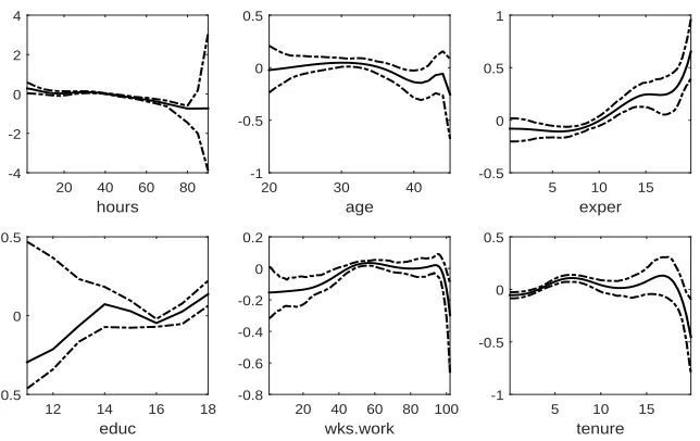
[Figure 3 about here.]
Figure 3 exhibits the estimated nonparametric functions in model (14) by using spline
approximations, in which the solid curves are the estimated nonparametric functions and the
dashed curves are the corresponding 95% pointwise confidence bands constructed using the
wild bootstrap procedure proposed by H¨ardle et al.(2004). Figure 3 shows thathours, one’s
usual hours worked, appears to be linearly and negatively correlated to the response variable
lwage, the level of one’s salary. The variable age, which represents one’s age in current
year, has a slight wavy dynamic effect, specifically an increase in lwage before 30 years old
and a decline after 35 are observed. On the other hand, exper, the total work experience,
has a relatively significant effect of increasing one’s wage at an increasing rate. As well, a
increase inwks.work, the weeks worked last year, generally raises one’s salary even though it
seems trifling. Similarly we observe thattenure, the years of job tenure, increases the value
oflwagewith some slight fluctuations though, particularly when the years of tenure is larger
than 18 or so. The SCAD-based selecting process identifies the variables hours, age, educ
for the parametric component and the variables exper and tenure for the nonparametric
component of the model, while the variable wks.work exerts no significant effect on the
level of salary. The estimated nonparametric functions using the SCAD penalty are shown
in Figure 4. There are similarities between the results shown in Figure 4 and Figure 3, for
example, the estimated function ofα5(exper) with SCAD penalization shows that the larger
value ofexper, the higher level of salary one can derive; also, by using SCAD selection, the
results show that an increase in the years of tenure can enhance the level of one’s salary until
the time of retirement.
[Figure 4 about here.]
[Table 4 about here.]
The results on autoregressive coefficients are reported in Table 4, where EST, SE and CI
denote the coefficient estimate corresponding to the parameters shown on the first column
of the table, its standard error, and the associated bootstrap-based 95% confidence interval.
Three sets of resulting results are presented: those without the implementation of SCAD or
other diagnostic tests are shown on the far left panel of the table; the middle panel presents
the re-estimated results after removing the insignificant variables based on t-test; the far
right panel are results based on the SCAD penalized procedure. The results without variable
selection by SCAD shows that s = 2 should be the appropriate autoregressive order in the
error structure, while the SCAD-based procedure provides a different choice with s = 3.
Specifically the similarity of both procedures is that the estimates of a1 and a2 are positive
and significant, and that ofb1 negative and significant. This suggests that one’s salary level,
after adjusting for the covariates within the same subject, are positively correlated, and that
the correlation tends to decrease as the observed time distance increases. On the other hand,
t-test and also agrees with the scatter diagrams in Figure 1 even though the dependence
seems much weaker.
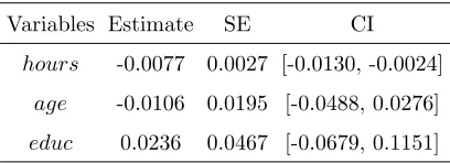
Table 5 below reports the identified parametric estimates of hours, age and educ, the
corresponding standard error and their bootstrap-based 95% confidence intervals. The
variable educinfluences the level of salary positively whileage has negative effect on lwage,
both of which agree with the intuition and also indicate that young people highly educated
are main force of the labour market. The more important is that the variable hours is
negatively correlated to one’s wage significantly from point of statistics, which implies that
one person has to take more time for earning money if his/her level of salary is too low,
although it just has minor effect on the improvement of living conditions. This perhaps
accurately reflects the social reality in those days.
[Table 5 about here.]
5
Discussion
To analyze the National Longitudinal Surveys (NLS) data, we employed a new
semiparametric longitudinal mean-covariance model in which the effects on dependent
variable of some explanatory variables are linear and others are nonlinear, while the
within-subject correlations were modeled by a non-stationary autoregressive error structure. We
constructed consistent estimators for both the parametric and nonparametric components
and established their asymptotic properties. In addition, a data-driven model selecting
procedure was proposed to identify the true effects of regressors on the response variable,
which was also applied to a real data analysis. However, the proposed linear structure of the
error component is perhaps not robust to outliers and in the risk of model misspecification.
Therefore, how to deal with such an issue is probably an interesting avenue of our future
Acknowledgements
We would like to thank the editor, the associate editor and two anonymous referees for their
constructive comments and suggestions. Li’s research was sponsored by National Statistical
Science Research Project(No.2016LZ22) and Shanghai Pujiang Program (No.16PJC042).
You’s research was supported by grants from the National Natural Science Foundation
of China (NSFC) (No.11471203) and Program for Innovative Research Team of Shanghai
University of Finance and Economics (IRTSHUFE). The work is also partially supported
by the Program for Changjiang Scholars and Innovative Research Team in University
(IRT13077).
Supporting information
Additional information for this article is available online including several assumptions
and lemmas used for establishing the asymptotic properties of resultant estimates and the
corresponding technical details in proof.
References
Bai, Y., Huang, J., Li, R. & You, J. (2015). Semiparametric longitudinal model with irregular
time autoregressive error process. Statist. Sinica 25(2), 507–527.
Cheng, G., Zhou, L. & Huang, J. Z. (2014). Efficient semiparametric estimation in generalized
partially linear additive models for longitudinal/clustered data.Bernoulli 20(1), 141–163.
Cochrane, D. & Orcutt, G. H. (1949). Application of least squares regression to relationships
containing autocorrelated error terms.J. Amer. Statist. Assoc. 44, 32–61.
De Boor, C. (1978). A practical guide to splines. Springer, New York. USA.
Diggle, P. J., Heagerty, P., Liang, K. Y. & Zeger, S. L. (2013). Analysis of longitudinal data.
Fan, J., Huang, T. & Li, R. Z. (2007). Analysis of longitudinal data with semiparametric
estimation of covariance function.J. Amer. Statist. Assoc. 102, 632–641.
Fan, J. & Li, R. (2001). Variable selection via penalized likelihood. J. Amer. Statist. Assoc.
95, 1348–1360.
Fan, J. & Li, R. (2004). New estimation and model selection procedures for semiparametric
modeling in longitudinal data analysis.J. Amer. Statist. Assoc. 99, 710–723.
Fan, J. & Wu, Y. C. (2008). Semiparametric estimation of covariance matrixes for
longitudinal data.J. Amer. Statist. Assoc. 103, 1520–1533.
Fan, Y. & Li, Q. (2003). A kernel-based method for estimating additive partially linear
models. Statist. Sinica, 739–762.
H¨ardle, W., Huet, S., Mammen, E. & Sperlich, S. (2004). Bootstrap inference in
semiparametric generalized additive models. Econom. Theory 20(02), 265–300.
He, X., Fung, W. K. & Zhu, Z. (2005). Robust estimation in generalized partial linear models
for clustered data. J. Amer. Statist. Assoc. 100, 1176–1184.
He, X., Zhu, Z. & Fung, W. (2002). Estimation in a semiparametric model for longitudinal
data with unspecified dependence structure. Biometrika 89, 579–590.
Hoover, D. R., Rice, J. A., Wu, C. O. & Yang, L. P. (1998). Nonparametric smoothing
estimates of time-varying coefficient models with longitudinal data. Biometrika 85(4),
809–822.
Huang, J.H., Wu, C. O. & Zhou, L. (2004). Polynomial spline estimation and inference for
varying coefficient models with longitudinal data.Statist. Sinica 14, 763–788.
Leng, C., Zhang, W. & Pan, J. (2010). Semiparametric mean-covariance regression analysis
for longitudinal data. J. Amer. Statist. Assoc. 105, 181–193.
Levin, A., Lin, C. F. & Chu, C. S. J. (2002). Unit root tests in panel data: asymptotic and
Liang, K. Y. & Zeger,S. (1986). Longitudinal data analysis using generalized linear models.
Biometrika 73, 13–22.
Lian, H., Liang, H. & Wang, L. (2014). Generalized additive partial linear models for
clustered data with diverging number of covariates using GEE.Statist. Sinica 24, 173–196.
Lin, D.Y. & Ying, Z. (2001). Semiparametric and nonparametric regression Analysis of
longitudinal data.J. Amer. Statist. Assoc. 96, 103–126.
Lin, X. & Carroll, R. (2001a). Semiparametric regression for clustered data using generalized
estimating equations.J. Amer. Statist. Assoc. 96, 1045–1056.
Lin, X. & Carroll, R. (2001b). Semiparametric regression for clustered data.Biometrika 88,
1179–1185.
Liu, X., Wang, L. & Liang, H. (2011). Estimation and variable selection for semiparametric
additive partially linear models.Statist. Sinica 21, 1225–1248.
Li, Y.H. (2011). Efficient semiparametric regression for longitudinal data with nonparametric
covariance estimation.Biometrika 98, 355–370.
MaCurdy, T. E. (1982). The use of time series processes to model the error structure of
earnings in a longitudinal data analysis.J. Econom. 18(1), 83–114.
Maddala, G. S. & Wu, S. (1999). A comparative study of unit root tests with panel data
and a new simple test.Oxford Bulletin of Economics and Statistics 61(S1), 631–652.
Ma, S. J., Song, Q. X. & Wang, L. (2013). Simultaneous variable selection and estimation
in semiparametric modeling of longitudinal/clustered data.Bernoulli 19, 252–274.
Pourahmadi, M. (1999). Joint mean–covariance models with applications to longitudinal
data: unconstrained parameterisation.Biometrika 86, 677–690.
Rice, J. A. & Silverman, B. W. (1991). Estimating the mean and covariance structure
nonparametrically when the data are curves.J. R. Stat. Soc. Ser. B., 233–243.
Rice, J. A. & Wu, C. O. (2001). Nonparametric mixed effects models for unequally sampled
Schumaker, L. L. (1981). Spline functions: Basic theory. Pure and applied Mathematics. A
Wiley–Interscience Publication. John Wiley & Sons, Inc., New York. USA.
Wang, H., Li, B. & Leng, C. (2009). Shrinkage tuning parameter selection with a diverge
number of parameters.J. R. Stat. Soc. Ser. B. 71, 671–683.
Wang, H., Li, R. & Tsai, C. (2007). Tuning parameter selectors for the smoothly clipped
cbsulote deviation method.Biometrika 94, 553–568.
Wang, L., Li, H. & Huang, J. H. (2008). Variable selection in nonparametric
varying-coefficient models for analysis of repeated measurements. J. Amer. Statist. Assoc. 103,
1556–1569.
Wang, L. & Yang, L. (2007). Spline-backfitted kernel smoothing of nonlinear additive
autoregression model.Ann. Statist. 35(6), 2474–2503.
Wang, N. (2003). Marginal nonparametric kernel regression accounting for within–subject
correlation.Biometrika 90, 43–52.
Wang, N., Carroll, R. & Lin, X. (2005). Efficient semiparametric marginal estimation for
longitudinal/clustered data.J. Amer. Statist. Assoc. 100, 147–157.
Wu, W. B. & Pourahmadi, M. (2003). Nnonparametric estimation of large covariance
matrices of longitudinal data.Biometrika 90, 831–844.
Zhang, H. H., Cheng, G. & Liu, Y. (2011). Linear or nonlinear? Automatic structure
discovery for partially linear models.J. Amer. Statist. Assoc. 106, 1099–1112.
Zhang, W. & Leng, C. (2012). A moving average Cholesky factor model in covariance
modeling for longitudinal data.Biometrika 99, 141–150.
Zhou, J. H. & Qu, A. (2012). Informative estimation and selection of correlation structure
for longitudinal data. J. Amer. Statist. Assoc. 107, 701–710.
Zou, H. & Li, R. (2008). One-step sparse estimates in nonconcave penalized likelihood
Rui Li, School of Statistics and Information, Shanghai University of International Business
and Economics, 1900 Wenxiang Road, Shanghai 201620, China.
The fitted error ǫ i,j-1
-2 0 2
The fitted error
ǫ i,j -2 -1 0 1 2
The fitted error ǫ i,j-2
-1 0 1 2
The fitted error
ǫ i,j -2 -1 0 1 2
The fitted error ǫ i,j-3
-2 0 2
The fitted error
ǫi,j -2 -1 0 1 2 (year
i,j-yeari,j-1)ǫi,j-1
-0.5 0 0.5
The fitted error
ǫ i,j -2 -1 0 1 2 (year
i,j-yeari,j-2)ǫi,j-2
-1 0 1
The fitted error
ǫ i,j -2 -1 0 1 2 (year
i,j-yeari,j-3)ǫi,j-3
-1 0 1
The fitted error
[image:25.612.138.469.103.304.2]ǫi,j -2 -1 0 1 2
Figure 1: Scatter diagrams of the fitting residualbεi,j and its lagged termsεbi,j−r forr= 1,2,3.
1 2 3 4
RASE of estimated functions
0.05 0.1 0.15 0.2 0.25 0.3
Box-plots of functions (n=50,m=5)
1 2 3 4
RASE of estimated functions
0.02 0.04 0.06 0.08 0.1 0.12 0.14 0.16 0.18 0.2
Box-plots of functions (n=100,m=5)
1 2 3 4
RASE of estimated functions
0.02 0.04 0.06 0.08 0.1 0.12 0.14 0.16 0.18
Box-plots of functions (n=150,m=5)
1 2 3 4
RASE of estimated functions
0.02 0.04 0.06 0.08 0.1 0.12 0.14 0.16 0.18
Box-plots of functions (n=50,m=10)
1 2 3 4
RASE of estimated functions
0.02 0.04 0.06 0.08 0.1 0.12
Box-plots of functions (n=100,m=10)
1 2 3 4
RASE of estimated functions
0.02 0.04 0.06 0.08 0.1 0.12
Box-plots of functions (n=150,m=10)
Figure 2: Boxplots of RASEs in Example 1: ’1’ denotes the estimator ˜α1,N(·) assuming the
errors are i.i.d and ’2’ is the proposed estimator αb1,N(·); ’3’ and ’4’ are similarly defined for
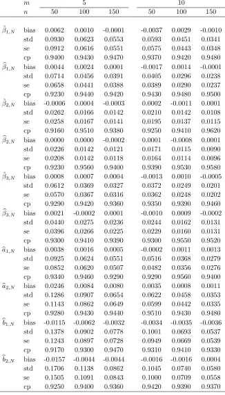
[image:25.612.114.496.427.627.2]Table 1: Finite results in Example 1: “bias” and “std” denote the average estimating bias and standard deviation of the parametric estimators, while “se” is average standard error and “cp” denotes the empirical coverage probability of 95% confidence intervals.
m 5 10
n 50 100 150 50 100 150
˜
β1,N bias 0.0062 0.0010 -0.0001 -0.0037 0.0029 -0.0010
std 0.0930 0.0623 0.0553 0.0593 0.0451 0.0341
se 0.0912 0.0616 0.0551 0.0575 0.0443 0.0348
cp 0.9400 0.9430 0.9470 0.9370 0.9420 0.9480
b
β1,N bias 0.0044 0.0024 0.0001 -0.0017 0.0014 -0.0001
std 0.0714 0.0456 0.0391 0.0405 0.0296 0.0238
se 0.0658 0.0441 0.0388 0.0389 0.0290 0.0237
cp 0.9230 0.9440 0.9420 0.9430 0.9480 0.9500
˜
β2,N bias -0.0006 0.0004 -0.0003 0.0002 -0.0011 0.0001
std 0.0262 0.0166 0.0142 0.0210 0.0142 0.0108
se 0.0258 0.0167 0.0141 0.0195 0.0137 0.0115
cp 0.9160 0.9510 0.9380 0.9250 0.9410 0.9620
b
β2,N bias 0.0000 0.0000 -0.0002 0.0001 -0.0008 0.0001
std 0.0226 0.0142 0.0121 0.0171 0.0115 0.0090
se 0.0208 0.0142 0.0118 0.0164 0.0114 0.0096
cp 0.9230 0.9560 0.9400 0.9390 0.9530 0.9580
˜
β3,N bias 0.0008 0.0007 0.0004 -0.0013 0.0010 -0.0005
std 0.0612 0.0369 0.0327 0.0372 0.0249 0.0201
se 0.0570 0.0367 0.0316 0.0362 0.0248 0.0202
cp 0.9290 0.9420 0.9360 0.9350 0.9390 0.9460
b
β3,N bias 0.0021 -0.0002 0.0001 -0.0010 0.0009 -0.0002
std 0.0440 0.0275 0.0236 0.0244 0.0162 0.0131
se 0.0396 0.0266 0.0225 0.0229 0.0160 0.0131
cp 0.9300 0.9410 0.9390 0.9300 0.9550 0.9520
ba1,N bias 0.0038 0.0016 0.0005 -0.0002 0.0011 0.0013
std 0.0925 0.0624 0.0551 0.0516 0.0368 0.0279
se 0.0852 0.0620 0.0507 0.0482 0.0356 0.0276
cp 0.9340 0.9460 0.9290 0.9290 0.9560 0.9400
ba2,N bias 0.0246 0.0084 0.0080 0.0035 0.0008 0.0011
std 0.1286 0.0907 0.0654 0.0622 0.0458 0.0353
se 0.1143 0.0862 0.0649 0.0599 0.0442 0.0335
cp 0.9280 0.9430 0.9440 0.9510 0.9430 0.9480
bb1,N bias -0.0115 -0.0062 -0.0032 -0.0034 -0.0035 -0.0036
std 0.1378 0.0902 0.0778 0.1001 0.0693 0.0537
se 0.1243 0.0897 0.0728 0.0949 0.0669 0.0539
cp 0.9170 0.9300 0.9470 0.9310 0.9410 0.9330
bb2,N bias -0.0157 -0.0044 -0.0044 -0.0016 -0.0016 0.0004
std 0.1706 0.1138 0.0862 0.1045 0.0740 0.0580
se 0.1505 0.1091 0.0843 0.1000 0.0709 0.0558
Table 2: Finite results in Example 2: “bias” and “std” denote the average estimating bias and standard deviation of the parametric estimators, while “Mean” and “Std” denote the empirical average RASEs and their standard deviations of the nonparametric estimators.
m 5 10
n 50 100 50 100
εi,j=ei,j
b
β1,N bias -0.0026 (-0.0030) -0.0002 (-0.0002) 0.0008 (0.0008) -0.0003 (0.0000)
std 0.0556 (0.0568) 0.0407 (0.0415) 0.0393 (0.0399) 0.0276 (0.0277)
b
β2,N bias 0.0037 (0.0033) -0.0028 (-0.0031) 0.0022 (0.0021) 0.0024 (0.0024)
std 0.0679 (0.0691) 0.0468 (0.0473) 0.0441 (0.0447) 0.0308 (0.0309)
b
α1,N Mean 0.1735 (0.1772) 0.1269 (0.1280) 0.1287 (0.1296) 0.0967 (0.0973)
Std 0.0430 (0.0440) 0.0290 (0.0294) 0.0275 (0.0281) 0.0181 (0.0183)
b
α2,N Mean 0.1641 (0.1672) 0.1131 (0.1144) 0.1152 (0.1165) 0.0806 (0.0810)
Std 0.0440 (0.0442) 0.0311 (0.0312) 0.0303 (0.0305) 0.0226 (0.0228)
εi,j= 1.5−∆ti,j,1−0.5(∆ti,j,1)2+ei,j
b
β1,N bias 0.0060 (-0.0023) -0.0013 (0.0014) 0.0010 (0.0028) -0.0017 (-0.0017)
std 0.0368 ( 0.0407) 0.0243 (0.0266) 0.0262 (0.0270) 0.0181 ( 0.0186)
b
β2,N bias 0.0002 (-0.0075) -0.0009 (-0.0014) -0.0008 (0.0027) 0.0008 (0.0029)
std 0.0255 ( 0.0325) 0.0194 ( 0.0200) 0.0214 (0.0180) 0.0112 (0.0119)
b
α1,N Mean 0.0897 (0.0916) 0.0758 (0.0795) 0.0725 (0.0709) 0.0610 (0.0620)
Std 0.0187 (0.0165) 0.0107 (0.0106) 0.0075 (0.0074) 0.0044 (0.0041)
b
α2,N Mean 0.0734 (0.0763) 0.0520 (0.0534) 0.0440 (0.0441) 0.0307 (0.0316)
Std 0.0200 (0.0205) 0.0145 (0.0145) 0.0123 (0.0116) 0.0081 (0.0085)
εi,j= exp(−∆ti,j,1) +ei,j
b
β1,N bias -0.0014 (0.0022) 0.0003 (0.0028) 0.0010 (0.0018) -0.0035 (0.0000)
std 0.0567 (0.0607) 0.0418 (0.0434) 0.0262 (0.0294) 0.0183 (0.0210)
b
β2,N bias 0.0000 (0.0005) -0.0003 (0.0044) -0.0008 (-0.0034) -0.0018 (-0.0030)
std 0.0451 (0.0461) 0.0307 (0.0316) 0.0214 (0.0226) 0.0141 (0.0149)
b
α1,N Mean 0.1204 (0.1262) 0.0939 (0.0973) 0.0745 (0.0803) 0.0655 (0.0673)
Std 0.0278 (0.0296) 0.0178 (0.0186) 0.0102 (0.0123) 0.0055 (0.0062)
b
α2,N Mean 0.1112 (0.1136) 0.0786 (0.0817) 0.0509 (0.0582) 0.0367 (0.0380)
Std 0.0312 (0.0320) 0.0209 (0.0227) 0.0141 (0.0161) 0.0098 (0.0101)
εi,j= Σ2r=1(ar+br∆ti,j,r) +ei,j
b
β1,N bias 0.0015 (0.0021) 0.0005 (-0.0025) 0.0002 (0.0020) 0.0011 (0.0040)
std 0.0487 (0.0530) 0.0318 (0.0393) 0.0318 (0.0416) 0.0227 (0.0286)
b
β2,N bias 0.0040 (0.0019) -0.0032 (-0.0024) -0.0010 (0.0026) 0.0005 (0.0005)
std 0.0420 (0.0475) 0.0275 (0.0339) 0.0222 (0.0312) 0.0147 (0.0196)
b
α1,N Mean 0.1174 (0.1321) 0.0894 (0.1021) 0.0754 (0.0887) 0.0633 (0.0737)
Std 0.0240 (0.0309) 0.0165 (0.0198) 0.0114 (0.0155) 0.0066 (0.0093)
b
α2,N Mean 0.1009 (0.1249) 0.0681 (0.0900) 0.0559 (0.0706) 0.0383 (0.0500)
Table 3: Model selection results: “U” denotes the number of under-estimated model, “C” the number of correctly estimated, and “O” denotes the number of over-estimated model.
Mean Error Mean+Error
Nonparametric Parametric
m n U C O U C O U C O U C O
10 50 141 547 312 224 623 153 96 841 63 178 487 335
100 0 825 175 67 908 24 0 988 12 0 758 242
150 0 893 107 51 930 19 0 999 1 0 823 177
15 50 99 671 230 139 704 157 8 967 25 195 573 232
100 0 941 59 23 943 34 0 998 2 0 928 72
150 0 973 27 11 965 24 0 1000 0 0 941 59
hours
20 40 60 80
-4 -2 0 2 4
age
20 30 40
-1 -0.5 0 0.5
exper
5 10 15
-0.5 0 0.5 1
educ
12 14 16 18
-0.5 0 0.5
wks.work
20 40 60 80 100
-0.8 -0.6 -0.4 -0.2 0 0.2
tenure
5 10 15
-1 -0.5 0 0.5
[image:28.612.147.469.403.606.2]exper
5 10 15
-0.2 -0.1 0 0.1 0.2 0.3 0.4 0.5 0.6 0.7 0.8
tenure
5 10 15
[image:29.612.174.441.83.220.2]-1 -0.5 0 0.5
[image:29.612.75.541.378.540.2]Figure 4: Fitting curves of the estimated nonparametric functions (solid line) together with their bootstrap-based 95% pointwise confidence intervals (dashed line) with SCAD identification.
Table 4: Estimated auto-regressive coefficients in the NLS data analysis and their standard errors (SE) and 95% confidence intervals (CI).
Estimates without SCAD Estimates without SCAD Estimates with SCAD
(removing insignificant variables)
EST SE CI EST SE CI EST SE CI
a1 0.8002 0.1168 [ 0.5713, 1.0291] 0.6702 0.0634 [ 0.5458, 0.7945] 0.7432 0.0841 [ 0.5785, 0.9080]
a2 0.3748 0.1860 [ 0.0102, 0.7394] 0.1963 0.0892 [ 0.0215, 0.3711] 0.2780 0.1198 [ 0.0433, 0.5128]
a3 -0.4347 0.5878 [-1.5869, 0.7175] – – – -0.2807 0.3386 [-0.9444, 0.3829]
a4 0.1008 0.5144 [-0.9075, 1.1090] – – – – – –
b1 -1.3930 0.2396 [-1.8626, -0.9233] -0.7307 0.2992 [-1.3171, -0.1443] -0.8958 0.1568 [-1.2031, -0.5886]
b2 -0.6207 0.2945 [-1.1980, -0.0435] 0.0588 0.2542 [-0.4393, 0.5570] -0.1990 0.3974 [-0.9779, 0.5798]
b3 0.7965 0.5663 [-0.3135, 1.9066] – – – 0.5820 0.3173 [-0.0399, 1.2039]
b4 0.1489 0.4849 [-0.8015, 1.0993] – – – – – –
Table 5: Estimates of identified parametric component in the NLS data analysis, the corresponding standard errors (SE) and 95% confidence intervals (CI).
Variables Estimate SE CI
hours -0.0077 0.0027 [-0.0130, -0.0024]
age -0.0106 0.0195 [-0.0488, 0.0276]
[image:29.612.204.408.631.705.2]