warwick.ac.uk/lib-publications
Original citation:
Pascali, Luigi (2017) The wind of change : maritime technology, trade and economic development. American Economic Review, 107 (9). pp. 2821-2854.
doi:10.1257/aer.20140832
Permanent WRAP URL:
http://wrap.warwick.ac.uk/83714
Copyright and reuse:
The Warwick Research Archive Portal (WRAP) makes this work by researchers of the University of Warwick available open access under the following conditions. Copyright © and all moral rights to the version of the paper presented here belong to the individual author(s) and/or other copyright owners. To the extent reasonable and practicable the material made available in WRAP has been checked for eligibility before being made available.
Copies of full items can be used for personal research or study, educational, or not-for-profit purposes without prior permission or charge. Provided that the authors, title and full
bibliographic details are credited, a hyperlink and/or URL is given for the original metadata page and the content is not changed in any way.
Publisher’s statement Copyright © 2016 AEA
https://www.aeaweb.org/journals/policies/copyright
A note on versions:
The version presented here may differ from the published version or, version of record, if you wish to cite this item you are advised to consult the publisher’s version. Please see the ‘permanent WRAP URL’ above for details on accessing the published version and note that access may require a subscription.
The Wind of Change: Maritime Technology, Trade and Economic
Development
Luigi Pascali
Pompeu Fabra University, University of Warwick, CAGE, and Barcelona GSE
October 12, 2016
Abstract
The 1870-1913 period marked the birth of the …rst era of trade globalization. How did this tremendous increase in trade a¤ect economic development? This work isolates a causality channel
by exploiting the fact that the introduction of the steamship in the shipping industry produced an
asymmetric change in trade distances among countries. Before this invention, trade routes depended on wind patterns. The steamship reduced shipping costs and time in a disproportionate manner
across countries and trade routes. Using this source of variation and novel data on shipping, trade,
and development, I …nd that 1) the adoption of the steamship had a major impact on patterns of trade worldwide, 2) only a small number of countries, characterized by more inclusive institutions, bene…ted
from trade integration, and 3) globalization was the major driver of the economic divergence between
the rich and the poor portions of the world in the years 1850-1905.
JEL:F1, F15, F43, O43
Keywords:Steamship, Gravity, Globalization, Trade, Development
1
Introduction
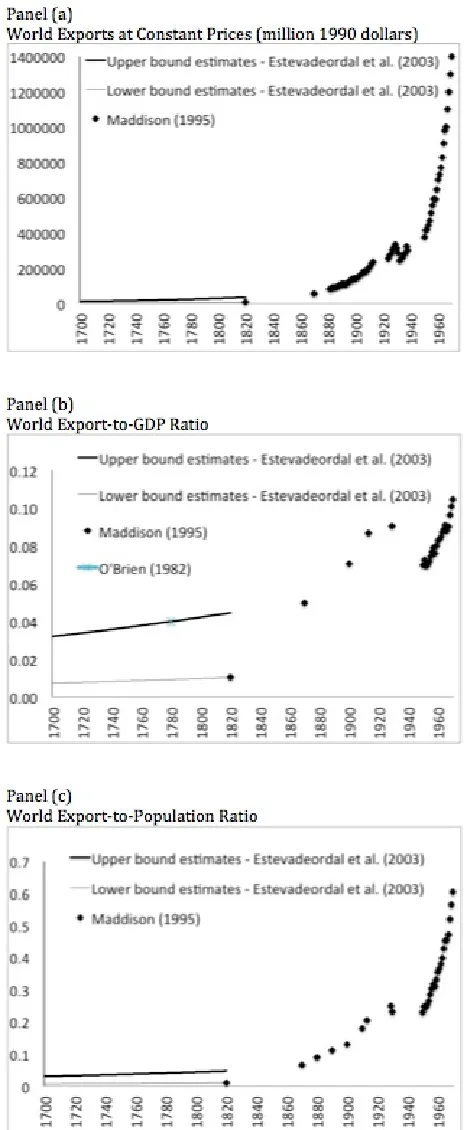
The 1870-1913 period marked the birth of the …rst era of trade globalization. As shown in Figure (1),
between 1820 and 1913, the world experienced an unprecedented increase in world trade, with a marked
acceleration that began in 1870. This increase in trade cannot simply be explained by increased global
GDP or population. In fact, between 1870 and 1913, the world export-to-GDP ratio increased from 5
percent to 9 percent, while per-capita volumes more than tripled. The determinants and consequences
of this …rst wave of globalization have been of substantial interest to both economists and historians.
This study employs new trade data and a novel identi…cation strategy to empirically investigate 1) the
role of the adoption of the steamship in shaping the pattern of world trade in the nineteenth century
and 2) the e¤ect of this tremendous increase in world trade on economic development.
This paper isolates a causality channel by exploiting the fact that the steamship produced an
asymmetric change in shipping times across countries. Before the invention of the steamship, trade
routes depended on wind patterns. The adoption of the steam engine reduced shipping times in a
disproportionate manner across countries and trade routes. For instance, because the winds in the
Northern Atlantic Ocean follow a clockwise pattern, the duration of a round trip for a clipper ship from
Lisbon to Cape Verde would be similar to that of a round trip from Lisbon to Salvador. However, with
the steamship, the former trip would require only half of the time needed for the latter trip. These
asymmetric changes in shipping times across countries are used to identify the e¤ect of the adoption
of the steamship on trade patterns and volumes and to explore the e¤ect of international trade on
economic development.
This paper is based on a large collection of data, as it uses three completely novel datasets that
span the great majority of the world from 1850 to 1900. The …rst dataset provides information on
shipping times using di¤erent sailing technologies across approximately 16,000 country pairs. The
second dataset consists of more than 23,000 bilateral trade observations for nearly one thousand
distinct country pairs and sectoral-level export data pertaining to 36 countries. Finally, the third
dataset provides information on freight rates across 291 major shipping routes. These data are then
combined with a large dataset on logbooks of sailing voyages between the 18th and the 19th centuries
and more traditional resources on per-capita income, population density and urbanization rates.
Four key …ndings emerge from this analysis.
and 1900 reveal that trade patterns were shaped by shipping times by sail until 1860, by a weighted
average of shipping times by sail and steam between 1860 and 1875, and by shipping times by steam
thereafter. I also document that this shift in patterns of trade was the result of a change in relative
freight rates induced by the steamship.
Second, I provide a rough estimate of the impact of the steamship on world trade volumes. I
measure the geographical isolation of a country as the average shipping time from this country to the
remainder of the world, and I use country-level regressions to estimate the impact of the change in
isolation, induced by the steamship, on the change in trade volumes between 1850 and 1905. The
estimated elasticity is surprising large. Using a simple back-of-the-envelope calculation, I argue that
the reduction in shipping times induced by the steam engine might be responsible for approximately
half of the increase in international trade during the second half of the nineteenth century. Admittedly
this is a very crude estimate and it should be taken with a grain of salt, as it is based on the assumption
that the roll out of the steam was uniform across di¤erent countries and di¤erent products and it was
completely concluded by the end of the period of analysis.
Third, the predictions for bilateral trade generated by the regressions of trade on shipping times
by sail and steam vessels are then summed to generate a panel of overall trade predictions for 36
countries from 1850 to 1905 (I limit the analysis to countries for which data on total exports and
per-capita GDP are available). These predictions can be used as instruments in panel regressions of
trade on per-capita income, population density and urbanization rates, and the time series variation
of the instrument allows for the inclusion of time- and country-speci…c …xed e¤ects in the
second-stage regression. I …nd that the e¤ect of trade on development and urbanization is not necessarily
positive: the average impact, in the short run, of the …rst wave of trade globalization was a reduction
in per-capita GDP, population density and urbanization rates all over the world. This average e¤ect,
however, masks large di¤erences across groups of countries. In particular, an exogenous increase in
international trade produced di¤erent e¤ects depending on the initial levels of economic development:
it was detrimental in countries characterized by a per-capita GDP below the top 33th percentile in
1860, while it did not impact the economic performance of the richest countries. Using these estimates,
I argue that the majority of the economic divergence that is observed between the richest countries
and the rest of the world in the second-half of the nineteenth century can be attributed to the …rst
Finally, I …nd that the e¤ect of trade on economic development is bene…cial for countries that are
characterized by strong constraints on executive power, which is a distinct feature of the institutional
environment that has been demonstrated to favor private investment. Following the …rst wave of trade
globalization, these countries specialized in non-agricultural products and bene…tted from trade. More
speci…cally, an exogenous doubling in the export-to-GDP ratio reduced per-capita GDP growth rates
by more than one-third in countries characterized by an executive power with unlimited authority,
while it increased per-capita GDP growth rates by almost one-…fth in countries in which the executive
power was obliged to respond to several accountability groups. Moreover, the latter countries increased
the share of their exports in non-manufacturing goods by almost one-third (while this share did not
signi…cantly change for the rest of the sample). This result is relevant to the large stream of literature
that has argued that institutions are crucial to obtaining bene…ts from international trade, although
I still view it as preliminary and exploratory: with a sample of only 36 countries, it is indeed very
di¢ cult to pin down the precise channels and mechanisms through which trade a¤ects development
with a reasonable degree of certainty.
To the best of my knowledge, this study is the …rst work that quanti…es the e¤ects of the adoption
of the steamship on global trade volumes and economic development in a well-identi…ed empirical
framework. This work also contributes to several strands of the economic literature.
First, my …ndings contribute to the debate on the importance of reduced transportation costs in
spurring international trade during the …rst wave of globalization. The most widely held
perspec-tive on the nineteenth century is that while railroads were responsible for promoting within-country
integration, steamships served the same role in promoting cross-country integration (Frieden (2007);
James (2001)). However, this view is not re‡ected in the most recent empirical literature examining
the …rst wave of trade globalization (O’Rourke and Williamson (1999), Estervadeordal et al. (2003),
Jacks et al. (2011)). In particular, these studies have emphasized the role of income growth when
focusing on explaining the increase in absolute trade and the role of the combination of decreasing
transportation costs and the adoption of the gold standard when focusing on trade shares. The
typi-cal methodology applied in this stream of literature is to regress exports on freight rates and then to
calculate the share of the increase in trade after 1870 that can be explained by the contemporaneous
reduction in freight rates. Thus, my paper addresses a major identi…cation issue: freight rates are
eco-nomic activity or market structure. Additionally, my work is the …rst to extend the period of analysis
before 1870. This extended period is necessary to capture the transition period from sail to steam
vessels and to explain the sources of the structural break in trade data after 1870.
Second, my …ndings contribute to the debate on the e¤ects of trade on development. Although I am
not aware of any paper that identi…es a causal link in the nineteenth century, a large body of literature
has focused on more recent years. Beginning with the seminal work of Frankel and Romer (1999), a
large number of papers have attempted to identify a causal channel using a geographic instrument:
the point-to-point great circle distance across countries. Although this instrument is free of reverse
causality, it is correlated with geographic di¤erences in outcomes that are not generated through trade.
For instance, countries that are closer to the equator generally have longer trade routes and may
have low incomes because of unfavorable disease environments or unproductive colonial institutions.
Rodriguez and Rodrik (2000) and others have demonstrated that Frankel and Romer’s results are
not robust to the inclusion of geographic controls in the second stage. More recently, Feyrer (2009a)
and Feyrer (2009b) exploit two natural experiments: the closing of the Suez Canal between 1967 and
1975 and improvements in aircraft technology that generated asymmetric shocks in trade distances.
Feyrer …nds that an increase in trade exerts large positive e¤ects on economic development. My work
demonstrates that although trade has been proven to exert generally positive e¤ects on development
in the present day, this might have not been the case one century ago.
Third, my …ndings contribute to the theoretical debate between neoclassical trade theories, in
which comparative advantages are determined by technological di¤erences and factor endowments,
and new economic geography theories, in which countries derive part of their comparative advantage
from scale economies. Trade liberalization in the conventional Ricardian or Heckscher-Ohlin approach
allows countries to exploit their comparative advantage: greater integration may harm particular
interest groups but typically increases income in all countries. This view has been challenged by the
new economic geography theories (see, for instance, Krugman (1991), Matsuyama (1992), Krugman
and Venables (1995), Baldwin et al. (2001) and Crafts and Venables (2007)). Although production
has constant returns to scale in the neoclassical world, these theories are based on increasing returns
within …rms and in the economy more broadly. Speci…cally, production in agriculture is still modeled
with constant returns, whereas production in manufacturing shows increasing returns to scale. When
a process of industrial agglomeration that is bene…cial for countries that specialize in manufacturing
and might be detrimental to countries that specialize in agriculture. My empirical …ndings support
this second stream of literature, as the …rst wave of trade globalization, in the short-run, had positive
e¤ects for a small core of countries while exerting negative e¤ects for other countries. A similar
empirical result, but limited to Chinese provinces, can be found in Faber (2014), who shows that
connections to China’s National Truck Highway System (a major investment in highway connections
between the major Chinese cities carried out on in the period from 1992-2007) led to a reduction in
GDP growth among peripheral counties.
Finally, my …ndings speak to the signi…cant body of empirical literature, beginning with the
sem-inal contributions of Acemoglu et al. (2001), Engerman and Sokolo¤ (1994), and La Porta et al.
(1997)2, which has convincingly shown that strong institutions (e.g., with respect to shareholder pro-tection, the strength of contract enforcement and property rights) are critical for economic growth.
The closest paper in this sense is Acemoglu et al. (2005), which shows that the rise of Atlantic trade
between the sixteenth and the nineteenth centuries produced a large positive impact on per-capita
GDP and urbanization only in those European countries that were characterized by political
institu-tions that placed signi…cant checks on monarchy. Levchenko (2007) demonstrates that, in a model
containing di¤erences in contracting imperfections across countries, trade is bene…cial in countries
with the strongest institutions, while it might become detrimental in countries characterized by weak
institutions, which will specialize in those goods that are not "institutionally dependent". To the best
of my knowledge, my work presents the …rst assessment of this theory, and, together with the work
of Acemoglu, Johnson and Robinson, it provides an empirical basis for an additional channel through
which institutions a¤ect economic development.
This paper is structured as follows. Section 2 provides a description of the evolution of shipping
technology during the second half of the nineteenth century. Section 3 describes the construction of
shipping times, trade …gures and the other data used in the paper. Section 4 describes the e¤ects of the
introduction of the steamship in the shipping industry on global patterns and volumes of international
trade. Section 5 examines the e¤ect of trade on development and urbanization as well as the role of
2
From sail to steam
The nineteenth century marked an era of spectacular advancements in terms of economic integration
throughout the world. It is generally believed that while the construction of new railroads fostered
within-country economic integration, the introduction of steam vessels in the shipping industry
en-couraged cross-country integration. In fact, the great majority of international trade in this period
was conducted by sea (see Table (A.1) in the online appendix). The reductions in trade costs between
countries, however, were not uniform across trade routes. To illustrate the asymmetric e¤ects on
international patterns of trade induced by the shift from sail to steam, in what follows I describe the
two competing technologies and their evolution in the second half of the century.
2.1 The sailing vessels
Figure (2) provides a polar diagram of a clipper, a fast-sailing ship that had three or more masts
and a square rig and that was largely used for international trade during the nineteenth century. A
polar diagram is a compact means of graphing the relationship between the speed of a sailing vessel
and the angle and strength of the wind. A clipper cannot navigate against the wind similar to all
other sailing vessels, and it reaches its maximum speed when sailing downwind at 140 degrees o¤
the wind. Additionally, the wind speed a¤ects the speed of the vessel, which is maximized when the
wind is moving at 24 knots. Given this technology, the prevailing direction and speed of the winds
become important determinants shaping the main international trade routes. Figure (A.1) and (A.2)
in the online appendix present the prevailing wind patterns worldwide and in Europe, while Figure (4)
depicts a series of journeys made by British ships between 1800 and 1860 between England, Cape of
Good Hope and Java. For instance, the winds tend to follow a clockwise pattern in the North Atlantic;
thus, it is much easier to sail westward from Western Europe after traveling south to 30 N latitude and
reaching the "trade winds," thus arriving in the Caribbean, rather than traveling straight to North
America. The result is that trade systems historically tended to follow a triangular pattern among
Europe, Africa, the West Indies and the United States. Furthermore, because the South Atlantic
winds tend to blow counterclockwise, British ships would not sail directly southward to the Cape of
Good Hope; rather, they would …rst sail southwest toward Brazil and then move east to the Cape of
Good Hope at 30 S latitude.
trade distance between di¤erent ports and countries.
2.2 The steam vessels
The invention and subsequent development of the steamship represents a watershed event in maritime
transport. For the …rst time, vessels were not at the mercy of the winds, and trade routes became
independent of wind patterns.
The …rst steamship prototypes emerged in the early 1800s. In 1786, John Fitch built the …rst
steamboat, which subsequently operated in regular commercial service along the Delaware River. The
early steamboats were small wooden vessels that used low-pressure steam engines and paddle wheels.
The paddles were replaced by screw propellers and wooden hulls by iron hulls beginning in the 1840s.
Steam …rst displaced sail in passenger and intra-national trade. Ine¢ cient engines prevented
these early steamships from being used in international trade, as longer voyages meant that a greater
proportion of a ship’s capacity needed to be devoted to coal bunkers rather than cargo.
Engine e¢ ciency was increased substantially when Elder and Radolph patented their compound
engine in 1853, although its e¤ective use was delayed until the introduction of higher-pressure boilers
in the following decade. Graham (1956) documents the dramatic reduction in coal consumption during
the second half of the nineteenth century: coal consumption per horsepower per hour of the average
British steamship declined by more than half between 1855 and 1870 and it stabilized afterwards (see
Figure (A.4) in the online appendix). These improvements, in conjunction with the increase in the
number of bunkering deposits, made steamship technology competitive even in long-distance trade.
The transition was rapid. Figure (3) presents an aggregate representation of the transition from sail to
steam. In 1869, the tonnage of British steam vessels engaged in international trade cleared in English
ports surpassed that of British sailing vessels for the …rst time. Moreover, whereas sail powered more
than two-thirds of the tonnage of ships built in the 1860s, this percentage declined to 15 percent during
the early 1870s.
By the end of the 1880s, sailing vessels were still in use only in round-the-world trade, in Australian
trade and in trade to the west coast of the Americas. Finally, by 1910, the shift from sailing vessels to
3
Data
The aim of this article is to study 1) the impact of the adoption of the steamship on freight rates,
patterns of international trade and trade volumes throughout the world in the second half of the
nineteenth century 2) the impact of the increase in world trade, resulting from the adoption of this
new technology, on economic development 3) the role of institutions and sectoral specialization in
order to take full advantage from trade. To do this, a wealth of data are needed that are discussed in
this section. In particular, data on shipping times by sail and by steam are described in subsection 1,
data on freight rates in subsection 2, data on bilateral, sectoral and total trade in subsection 3, data
on economic development, population and urbanization in subsection 4, and data on institutions in
subsection 5. Tables (1) reports the summary statistics for this set of data.
3.1 Sailing times (optimized routes and actual voyages)
Optimized bilateral sailing times were calculated by the author. The world was divided into a matrix
of one-by-one degree squares. For each square, data downloaded from the Center for International
Earth Science Information Network (CIESIN)3were used to identify whether it was land or sea, while the US National Oceanic and Athmospheric Administration (NOAA) provided data on the average
velocity and direction of the sea-surface winds4.
The sailing time from each oceanic square to each of the eight adjacent squares on the grid was
determined by the velocity and direction of the wind along the path, according to the speci…c polar
diagram of the vessel. The world matrix was then transformed into a weighted, directed graph in which
every one-degree square is a node and the travel times to adjacent squares are the edges’weights.
Four graphs were constructed to account for the two sailing technologies (sail versus steam vessels)
and the inclusion/exclusion of the Suez Canal as a valid path. Given any two nodes in the graph, the
Djikstra’s algorithm was then used to compute the shortest travel time5.
After identifying the primary ports for each country, I calculated all pairwise minimum travel
times. Identifying the primary ports for each country was straightforward, and for the majority of
countries, the choice of port would not change the results. The exceptions were countries with the
longest coastlines and those bordering two or more oceans. For these countries, up to 5 primary ports
in 1850 were considered. The minimum travel time between two countries was then computed as the
The optimized routes by sail were compared with a set of actual voyages by sailing ships between
1742 and 1854 described in 3026 logbooks digitized in the CLIWOC dataset. For these voyages, the
logbooks report the starting point, the ending point and the duration in days (intermediate stops are
not recorded). Column 1 of Table (2) shows the results when regressing the duration of these voyages
on the travel times computed using the optimization algorithm. The coe¢ cient is positive, statistically
signi…cant (with a t-statistics of approximately 16) and above 1, re‡ecting the fact that the optimized
routes are direct routes, while actual routes might include intermediate stops (it should be noted that
the R-square of this regression is approximately 50%). In column 2, I add year …xed e¤ects: the
results are unchanged. The partial scatter plot for the regression in this column is presented in Figure
(A.3) in the online appendix. The results are also unchanged when controlling for geographic distance
across starting and ending port (columns 3 and 4). Finally, Figure (5) shows the optimized routes
by sailing vessels between England, Cape of Good Hope and Java. The accuracy of the optimization
is con…rmed by the fact that these optimal routes can perfectly reproduce the routes followed by the
actual journeys of British sailing ships shown in Figure (4), both in the Atlantic Ocean and in the
Indian Ocean6.
Tables (1 - PANELS: A and B) reports the summary statistics for this set of optimized shipping
times and the duration of the actual voyages in the CLIWOC dataset. It is noteworthy that the
introduction of the steamship reduced the average shipping time by more than half, and the opening
of the Suez Canal reduced this time by an additional ten percent.
3.2 Freight rates
A database on freight rates from the English ports of Newcastle and Cardi¤, covering the years
1855-1900, was constructed using three di¤erent sources.
The …rst source is the Newcastle Courant. This newspaper reported the freight rates for shipping
coal from Newcastle to 147 di¤erent ports weekly. I collected the shipping rates reported in the …rst,
second and third week of February in the years 1855-1870. These freight rates were then averaged
within each year-route, resulting in a total of 1,643 observations.
The second source is the Mitchell’s Maritime Register, a weekly journal of shipping and commerce.
This newspaper reported freight rates for shipping coal and iron in the years 1857-1883 from the
observations.
The last source is Angier (1920), which provides 1,010 observations of freight rates for coal and
iron from the ports of Cardi¤ and Newcastle from the years 1870-1913.
The entries from these three sources were then standardized and converted into shillings per ton.
Descriptive statistics are reported in Table (1 - PANEL B).
3.3 Trade data
A database for bilateral trade covering the entire second half of the nineteenth century was constructed
by the author from primary sources. Table (1 - PANEL C) reports the summary statistics for this
set of data. Overall, the data consist of almost 24 thousand bilateral trade observations for nearly
one thousand distinct country pairs. This database signi…cantly improves upon the trade data used in
prior studies of the nineteenth century, as it is better suited to identifying the impact of the steamship
on trade patterns and development, mainly because of its sheer size and time coverage. To date,
the most comprehensive bilateral trade database for this century is that constructed by Mitchener
and Weidenmier (2008), which covers 700 distinct country pairs for the 1870-1900 period7. My data are superior in both dimensions of the panel: the number of years and the country pairs. The most
signi…cant di¤erence is that my data cover the entire second half of the century, which is essential to
capturing the transition from sailing technology to steam. The list of countries with available bilateral
trade data are listed in Table (A.2) in the online appendix.
A large number of documents, listed in the online appendix, were used to assemble this dataset.
Trade data for this period are available from summary tables assembled by the di¤erent national
statis-tical institutes starting from national custom records. The great majority of the data (approximately
70 percent of the total entries) comes from the British Board of Trade Statistics. In particular, I rely
on four di¤erent annual publications published by this institution between 1850 and 1905: the
Statis-tical Abstract for the Principal Foreign Countries, the StatisStatis-tical Tables relating to Foreign Countries,
the Statistical Abstract for the Several British Colonies, Possessions, and Protectorates and the
Sta-tistical Abstract for the United Kingdom. The second largest share of entries (11 percent) comes from
the French Department of Foreign A¤airs and Trade, and particularly from two annual publications:
The Tableau Général du Commerce de la France avec ses colonies et les puissances étrangères and
historians rank British and French trade statistics as the best data available for the 19th century. A
complete discussion about their reliability can be found in Lampe (2008)8. The remaining share of the entries comes from datasets assembled by contemporary historians on single (e.g., Pamuk (2010))
or multiple countries (e.g., Mitchell (2007)) based on national customs data.
The trade dataset also comprises 332 entries on total exports and 234 entries on the share of exports
in non-agricultural products (36 countries every …ve years from 1845 to 1905, with gaps). In order
to construct the latter share, approximately half million entries on exports by product were collected
from primary sources; a SIC (rev1) code was then assigned to each of these products; and, …nally, the
share of exports that did not belong to the SIC categories 0 (food and live animals), 1 (beverages and
tobacco), 4 (animal and vegetables oils and fat) was computed. Descriptive statistics for the variable
total exports and share in nonagricultural products are reported in the …rst two rows of Table (1
-PANEL D).
All trade data were then converted into pounds sterling using annual exchange rates provided by
the British Board of Trade in numerous volumes of the Statistical Abstract for the Principal and Other
Foreign countries or by the Global Financial Database and Ferguson and Schularick (2006).
3.4 Per-capita GDP, population and urbanization rates
Data on per-capita income were obtained from the Maddison Project Database (Bolt and van Zanden
(2014)), which is a recently updated version of the original Maddison (2004) dataset, whereas the
population data come from a large number of di¤erent sources that are listed in the online appendix.
This study also uses two di¤erent measures of urbanization: the percentage of the population living
in cities with more than 50 and 100 thousand citizens. Urbanization rate data were readily available
for the majority of countries from the Cross-National Time-Series Data Archive (Banks and Wilson
(2013)). For the remaining 10 countries in the sample, city-level data on the number of residents
were obtained from a large number of sources (which are described in the online appendix) and then
aggregated at the country level.
The last four rows of Table (1 - PANEL D) report summary statistics on per-capita income, total
population and urban population. The data are available every 5 years for the period from 1845-1905
for 36 countries (see Table (A.3) in the online appendix for the list of countries with available aggregate
3.5 Institutions
An initial question concerns which aspect of political institutions should be the focus of the analysis.
Douglass North (1981) argues that high-quality institutions are a primary determinant of economic
performance because they serve two functions: supporting private contracts (contracting institutions)
and providing checks against expropriation by the government or other politically powerful groups
(property rights institutions). However, Acemoglu and Johnson (2005), in an attempt to determine
the relative roles of contracting institutions versus property rights institutions, …nd that only the
latter have a …rst-order e¤ect on long-term economic growth. For this reason, this paper will focus
on the quality of property rights institutions and use the variable “Constraints on the Executive,”
as de…ned in the dataset POLITY IV, to rank political institutions. This variable is designed to
capture “institutionalized constraints on the decision-making powers of chief executives.” According
to this criterion, better political institutions exhibit one or both of the following features: the holder of
executive power is accountable to bodies of political representatives or to citizens, and/or government
authority is constrained by checks and balances and by the rule of law. A potential disadvantage of
this measure is that it primarily concerns constraints on the executive while ignoring constraints on
expropriation by other elites, including the legislature. The variable “Constraints on the Executive”
varies from 1 (unlimited authority) to 7 (accountable executive constrained by checks and balances)
with higher values corresponding to better institutions. It is not available in the POLITY IV dataset
for eight countries that were not independent in 1860. For these countries (highlighted in Table (A.3)
in the online appendix), the score is therefore coded by the author.
4
The steamships and the e¤ects on trade
4.1 The shift from sail to steam
The historical literature on when the introduction of steam technology to maritime transportation
became relevant for international trade is divided. Graham (1956) and Walton (1970) argue that the
transition from sail to steam was a slow and protracted process and was the result of the continuous
improvements in the fuel consumption of marine engines that occurred throughout the second half of
the century. By contrast, Fletcher (1958) and Knauerhase (1968) argue that the transition occurred
the compound engine, whereas Fletcher posits that it was the catalytic e¤ect of the construction of
the Suez Canal in 1860, which was suitable for steam vessels but not for sailing vessels.
Rather than assuming a particular position in this debate, I will use a gravity-type regression to
determine when the distances in terms of the time to sail by steamship became relevant in explaining
patterns of trade worldwide. The gravity model is an empirical workhorse in the trade literature.
Practically, trade between two countries is inversely related to the distance between them and positively
related to their economic size. The following is a basic expression for bilateral trade:
ln(tradeijt) = ln(yit) + ln(yjt) + ln(ywt) + (1 ) ln( ijt+ lnPit+ lnPjt) +"ijt (1)
where tradeijt denotes the exports from country i to country j, yit and ywt are the GDP of country
i and of the world, ijt is the bilateral resistance term (and captures all pair-speci…c trade barriers
such as trade distance, common language, shared border, and colonial ties), and Pit and Pjt are the
country-speci…c multilateral resistance terms that are intended to capture a weighted average of the
trade barriers of a given country.
This speci…cation emerges from several micro-founded trade models (see, for instance, Anderson
and van Wincoop (2003) and Eaton and Kortum (2002)). These models typically imply a set of
predictions regarding trade diversion and trade creation. First, exports from i to j are increased when
the bilateral resistance term ijt declines relative to the multilateral resistance terms Pit and Pjt.
Second, as world trade is homogenous of degree zero in the bilateral resistance terms, international
trade will increase only when international frictions ijt and jit decline relative to intranational
frictions iit and jjt. Note that the introduction of the steamship was responsible for both a change
in the relative bilateral frictions across countries and a reduction in international frictions relative to
intranational frictions, as the steamship was utilized disproportionately more for international shipping
than for domestic shipping.
Although the majority of international trade is shipped by sea, the vast majority of estimated
gravity models assume that the bilateral resistance term is a function of point-to-point great circle
distances rather than navigation distances. By contrast, this paper assumes that this term is a function
ln(tradeijt) = steam;Tln(steamT IM Eij) + sail;Tln(sailT IM Eij) +Xijt + t+"ijt (2)
wheresteamT IM Eij and sailT IM Eij are the sailing times from country i to country j by steam and
sailing vessels, respectively, andXijtindexes a set of variables to control for the P and y terms in the
original gravity equation. Note that the coe¢ cients on the two distances are allowed to vary over time
to capture changes in the navigation technology from sail to steam.
The results of these regressions are presented in Table (3). Standard errors are 3-way clustered to
allow for arbitrary correlation within exporter, importer and year. The coe¢ cient on sailing times is
allowed to vary every 5 years. In the benchmark speci…cation, the P and y terms are controlled using
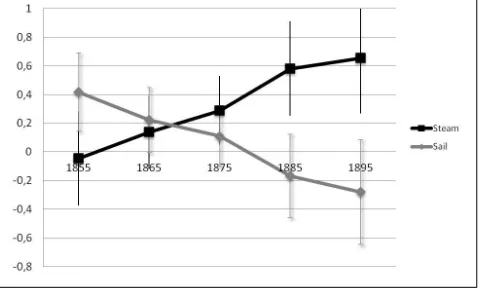
importer …xed e¤ects, exporter …xed e¤ects and year …xed e¤ects. Figure (6) plots the sequence of the
estimated coe¢ cients on shipping times (the error bars represent the 90 percent con…dence interval
around the point estimates). The coe¢ cient on shipping time by steam is close to zero and not
signi…cant until 1865, while it becomes negative, large and signi…cantly di¤erent than zero thereafter:
it decreases to -0.5 in the period from 1866-1870, to -0.7 in the period from 1871-1875 and it stays
at similar levels until 1900. In the same …gure, the coe¢ cient on shipping time by sail is negative
(between -0.7 and -0.6) until 1865, while it is very close to zero in the years thereafter. This evidence
is consistent with the view of a rapid change toward steam in the maritime transportation industry
that started in the late 1860s and was completed in the early 1880s9.
A potential concern with this speci…cation is that countries’relative sizes and multilateral resistance
change over time. If these relative changes are correlated with shipping distances by sail and steam,
then the estimates in Figure (6) may be biased. For this reason, I supplement this speci…cation with
importer-by-year …xed e¤ects and exporter-by-year …xed e¤ects. Figure (7) indicates that from a
qualitative perspective, the results are only slightly a¤ected. In a practical sense, the only di¤erence
is that in this new speci…cation, the coe¢ cient on shipping times by steam is positive and signi…cant
in 1860. This anomaly is consistent with the failure to reject a false null hypothesis with 5 percent
probability.
Finally, the coe¢ cients plotted in Figure (8) come from a regression that includes year and bilateral
pair dummies. In this case, the absolute level of the elasticities of sailing times cannot be captured;
standardized to 0. These estimates match the previous …ndings. Over time, country pairs that were
relatively closer by steam than by sail experienced the greatest increase in trade.10
Overall, these results corroborate the view that the introduction of the steamship in the shipping
industry was responsible for a substantial change in trade patterns in the second half of the nineteenth
century, with the majority of the change happening during the 1870s.
4.2 The steamship and the …rst wave of globalization
The previous section emphasized that the steamship reshaped global trade patterns beginning in
approximately 1870. Circa this period, per-capita international trade increased threefold. Is there
a causal link between these two observations? What extent of the increase in international trade is
explained by the shift from sail to steam in the maritime industry? Estervadeordal et al. (2003) argue
that a general equilibrium gravity model of international trade implies that 57 percent of the world
trade boom between 1870 and 1913 can be explained by income growth. The adoption of several
currency unions and declining freight rates each roughly account for one-third of the remaining part,
while the remainder is explained by income convergence and tari¤ reductions. A more recent work by
Jacks et al. (2011) corrects the estimates obtained by Estavadeordal et al. using a more comprehensive
dataset on freight rates for the same period and …nds the e¤ect of the maritime transport revolution
on the late nineteenth century global trade boom to be trivial. Other studies focus on global market
integration— the convergence of prices across markets— rather than on trade and trade shares. Jacks
(2006) presents evidence from a number of North Atlantic grain markets between 1800 and 1913 and
indicates that changes in freight costs can explain only a relatively modest fraction of the changes
in trade costs occurring in those markets. Using similar data, Federico and Persson (2007) conclude
that changes in trade policies were the single most important factor explaining the convergence and
divergence of prices in the long term.
All of the above-mentioned studies use changes in freight rates to proxy for changes in
transporta-tion costs. The disadvantage of this approach is that freight rates are simply prices for transport
services and, as such, are likely to respond not only to technology shocks but also to shifts in the
demand schedule for shipping services and changes in the market structure in the shipping industry.
Both of these confounding factors were present in 1870. First, the adoption of the gold standard,
shipping services. Second, beginning in the 1870s, rate schedules and shipping capacity for overseas
freight on a number of trade routes began to be established by shipping line conferences/cartels. Every
main trade route between regions had its own shipping conference organization composed of all the
shipping lines that served the route11.
Given the contemporaneous shift in the demand for shipping services and the change in market
structure, it is not surprising that the introduction of the steamship did not immediately translate
into a sharp reduction in the overall price of shipping services. For instance, the North’s freight index
of American export routes declined at the beginning of the nineteenth century and remained stable
between 1850 and 1880, whereas Harley’s British index declined more rapidly after 1850, well before
the introduction of the steamship on a major trade route. Neither index exhibited a structural break
between 1865 and 1880, although the number of steamers that were constructed increased signi…cantly
during this period, while the construction of larger sailing ships nearly ceased.12
In this section, I will measure the e¤ect of the introduction of the steamship on the trade boom
during the second half of the nineteenth century by relying on an actual measure of technological
improvement— the reduction in sailing times— rather than on freight rate indexes. This approach has
the key advantage that the change in sailing times is arguably exogenous with respect to the demand
for shipping services and the market structure in the shipping industry, as this change is the result of
prevailing wind patterns and ocean currents.
Table (4) reports estimates from the following regression:
ln(f reightijpt) = steam;T ln(steamT IM Eij) + sail;Tln(sailT IM Eij) +Xijpt + t+"ijpt (3)
wheref reightijptis the average freight rate from port i to port j for product p in year t;Xijptindexes
a set of control variables; and t are year …xed e¤ects that are supposed to capture common shocks
to freight rates. As in equation (2) the coe¢ cients on the two shipping times are allowed to vary
over time to capture changes in the navigation technology from sail to steam. Unfortunately data on
freight rates are not as comprehensive as data on exports: they are limited to outbound rates on 2
products - coal and iron - and only capture shipments from two UK ports - Cardi¤ and Newcastle - to
195 foreign ports (for a total of 291 routes) scattered over 33 di¤erent countries. To increase the power
years, as for the trade estimates in Table (3)).
The benchmark speci…cation, reported in column 1 of Table (4), controls for country of destination,
year and product …xed e¤ects. Voyage duration by steamship does not have a relevant impact on freight
rates in the 1850s and the 1860s, while it does have a positive and signi…cant impact thereafter. Voyage
duration by sailing ship instead has a positive impact in the …rst two decades but not thereafter. These
results are unchanged when controlling for great-circle distance between ports (column 2) and when
adding route …xed e¤ects (column 3), with the usual caveat that, in this latter case, the absolute level
of elasticities of sailing times cannot be captured.
In sum, the results in Table (4) prove that, although there was not a general sharp decline in
freight rates immediately after the di¤usion of the steamship, there was still a relative decline along
those routes in which the steamship had a larger impact on shipping times. To estimate the e¤ect
of the reduction in shipping times induced by the introduction of the steamship on the change in
international trade volumes, I then estimate the following regression:
logTi =c+ logDisti+ i (4)
wherecis the intercept, logTi is the log-change in either the export-to-GDP ratio or the per-capita
exports of country i between 1850 and 1905 and logDisti is the average change in shipping times
across all trading partners (weighted by their share of world trade) generated by the introduction of
the steamship:
logDisti P
j6=i
wj[ln(steamT IM Eij) ln(sailT IM Eij)] (5)
Figure (10) reports the di¤erent values of the logDisti variable, across all the polities of the world in
1900 that are not landlocked. (See the online appendix C for an in-depth discussion of the geographical
determinants of this variable).
The elasticity can be interpreted as the e¤ect of the introduction of the steamship on international
trade by reducing sailing time, under the assumption that all international trade was carried by sailing
vessels in 1850 and by steam vessels in 1905. Because a smaller portion of international trade was still
conducted by sail in 1905 or was shipped by land (or river), estimates of the e¤ects of the steamship
are likely to be downwardly biased.
benchmark speci…cation, reported in column 1, implies that the e¤ect of isolation on trade is negative
and highly signi…cant. Increasing the weighted average shipping time to the rest of the world from the
level of France to the level of Cuba implies a reduction in the export-to-GDP ratio of 74 log points
and in the export-to-population ratio of 133 log points. In columns 2, 3, 5 and 6 of Table (5), I limit
the weighted sailing distances to the top 5 and top 20 trading countries. It is clear that the qualitative
results do not vary according to the particular weights selected to aggregate sailing times across the
di¤erent trading partners. In all cases, the e¤ect of isolation remains negative and signi…cant, although
the estimated elasticity oscillates between -1.2 and -1.4 when the regressor is the export-to-GDP ratio
and between -1.6 and -1.8 when the regressor is per-capita exports. It should be noted that there
are more observations for the latter variable (54 versus 24) because we lack GDP data for the years
1850 and 1905 for a large number of countries. The result is that the OLS estimates are more precise
when using per-capita exports rather than the export-to-GDP ratio. In Table (5), the observations
are weighted by the log of the countries’total populations. Unweighted estimates are reported in the
appendix: the results are practically unchanged (see Table (A.5)).
These estimated elasticities can be used to produce a rough estimate of the role of the introduction
of steam vessels in spurring trade during the period of analysis. The population-weighted average
log-change in per-capita trade between 1850 and 1905 in my sample of countries is 1.4. If we assume
that the steamship in 1905 is, on average, 50 log-points faster than the sailing vessels active in 185013 then the most conservative estimates imply that the steamship might be responsible for at least half
(-0.5*-1.54/1.4=0.55) of the trade boom that occurred over these years14. This number is surprisingly large compared with the previous estimates described at the beginning of this section. However, as
usual in these back-of-the-envelope calculations, we should take it with a grain of salt, as it is based
on the assumption that the roll out of the steam was uniform across di¤erent countries and di¤erent
products and it was completely concluded by the end of the period of analysis.
To conclude, starting in 1865-1870, the introduction of the steamship reduced shipping times by
approximately one-half. This did not translate in an immediate reduction of average freight rates
following the introduction of the steamship because other confounding factors were, at the same time,
pushing freight rates in the opposite direction. A simple back-of-the-envelope calculation (which should
be taken cautiously) suggests that, the fact that the steamship was able keep freight rates on the low
5
Trade and Economic Development
The aim of this section is to evaluate the e¤ect of this trade boom in the second half of the nineteenth
century on economic development. The basic estimating equation is as follows:
log(Yit) = logTit+ i+ t+ it (6)
where Yit is per-capita GDP, and Tit is either the export-to-GDP ratio or the per-capita exports of
country i. To identify the causal e¤ect, this equation is estimated using 2SLS, instrumenting Tit
with the component of country i’s total exports that is explained by the geographic isolation of the
country as determined by the prevailing shipping technology in t. Speci…cally, I isolate the geographic
component of country i’s exports to its trade partner j in year t using the following formula:
logP Tijt=bsteam;tln(steamT IM Eij) +bsail;tln(sailT IM Eij) (7)
The geographic component of a country’s total exports is then computed as the weighted average
of these bilateral components across all of country i’s potential trading partners using the partners’
shares in total world trade as weights:
logP Tit=P
j6=i
wjlogP Tijt (8)
Note that the instrument for trade,logP Tit, is time varying. Within-country variation is generated
by the shift from sail to steam vessels, which induces a change in the bilateral shipping time across
countries and, through this channel, a shift in the relative level of geographic isolation of countries
worldwide. The time-varying nature of the instrument implies that, in contrast to the approach used
by Frankel and Romer, country …xed e¤ects can be added to equation (6).
Table (6) presents the OLS, 2SLS and reduced-form estimates of equation (6). Standard errors are
two-way clustered to allow arbitrary correlations within country and within year and they are corrected
to account for the fact that the instrument depends on the (estimated) parameters of the bilateral
trade equation15. The sample is an unbalanced panel that covers 36 countries with observations every 5 years from 1845 to 1905 (the exact countries and years available are illustrated in Figure (A.7) in
the measure of trade openness. Per-capita GDP is negatively correlated with the export-to-GDP ratio
and positively correlated with the export-to-population ratio. This anomaly is likely the result of a
spurious correlation of the denominators of the two regressors with the dependent variable. Columns
2 and 5 (3 and 6) report the unweighted (weighted) 2SLS estimates. In each case, the …rst stage
is strong. The Kleiberg-Paap F statistic for weak identi…cation exceeds 10, which is the standard
threshold for a powerful instrument as suggested by Staiger and Stock (1997). The impact of trade
openness on per-capita GDP is negative. An increase in the export-to-GDP (export-to-population)
ratio by 1 percent produces a reduction in per-capita GDP in the order of 0.18 (0.22) percent. Finally
columns 7 and 8 report the reduced-form estimates.
To understand which of the observations are driving the …rst stage and the reduced-form estimates,
Figures (A.8)-(A.10) in the appendix provide a simple scatter plot of the log-change in predicted trade,
P Tit,against the log-change in export rates and in per-capita GDP over the years 1850-190516. Figure (A.8) shows that there is a clear positive correlation between the log-change in the instrument and
the log-change in both the export-to-population and the export-to-GDP ratios. Figure (A.9) reports,
instead, the scatter plot of the log-change in the instrument against the log-change in per-capita
GDP: the two variables are negatively correlated. The main exceptions to this rule are four South
American republics: Brazil, Venezuela, Colombia and Uruguay. A potential explanation is that Latin
America had the highest tari¤s in the world from the late 1880s onward (Williamson, 1935 p. 204).
In these countries, shipping rates represented a small fraction of total trade costs, and the change in
freight rates induced by the steamship was unlikely to have had a large impact on total trade costs.
In Figure (A.9), Europe is clearly dominating the picture, as 13 out of 28 countries are European.
Moreover, European countries experienced the largest reduction in shipping times in this sample and
faced relatively low per-capita GDP growth rates (this is particularly true for Southern Europe). In
Figure (A.10), European countries are omitted: the correlation is still negative and the slope of the
regression line is practically unchanged. In this case, however, the correlation coe¢ cient drops by half
when excluding New Zealand and Dutch East Indie from the sample.
A potential concern with these estimates is that per-capita GDP might not be an ideal proxy of
economic development in a world that is largely still Malthusian. For this reason, in Table (7), I repeat
the analysis using population density and urbanization rates as alternative proxies. Trade again has
population density by 1.1 percent, the share of the population living in cities with more than 50
thousand citizens by 0.08 percent and the share living in cities with more than 100 thousand citizens
by 0.08 percent. The results are practically unchanged when using per-capita trade as a measure of
trade openness (see Table (A.7) in the appendix).
The …nding that the e¤ect of the …rst wave of globalization could be negative on average is
sur-prising. In a previous study, Williamson (2011) documents a negative correlation between growth in
terms of trade (generated by increased trade) and per-capita GDP growth in a large set of developing
countries between 1870 and 1939. However, to the best of my knowledge, the current study is the …rst
to document a negative causal e¤ect. Several authors (Lewis (1978), Williamson (2008), Williamson
(2011), Acemoglu et al. (2005) and Galor and Mountford (2008)) have related the …rst wave of trade
globalization to the Great Divergence, a term coined by Samuel Huntington to describe the 19th
cen-tury process by which the Western world overcame pre-modern growth constraints and emerged as
the most powerful and wealthy world civilization of the time. Table (8) examines the relationship
between trade and economic divergence17. The results are striking. An exogenous increase in inter-national trade produced di¤erent e¤ects depending on the initial levels of economic development: it
was detrimental in countries characterized by a per-capita GDP below the top 33th percentile in 1860,
while it did not impact the economic performance of rich countries (see columns 3, 4, 7 and 8).
Between 1870 and 1900, the export-to-GDP ratio increased at a yearly rate of 0.020, while
per-capita GDP increased at a rate of 0.008 (in the 43 countries for which per-per-capita GDP estimates
are available in the Maddison database). However, this average increase in per-capita GDP masks
important di¤erences as the top 14 richest countries in 1870 grew at a yearly rate of 0.013, while the
rest grew at a yearly rate of 0.005. Therefore, the gap in the growth rate between the richest 33 percent
and the rest was approximately 0.008. According to the estimates in Table (8), the …rst wave of trade
globalization was responsible for at least 79 percent (0.316*0.020/0.008) of this gap. The estimates in
Table (8) con…rm that international trade was the main force behind the Great Divergence. Moreover,
they tell us that to industrialize and bene…t from trade, it was not enough to start as rich because, on
average, rich countries did not lose from trade, but they also did not bene…t.
The question that naturally follows is whether the e¤ect of trade was negative everywhere or
whether certain countries actually bene…tted from trade. In the following tables, I turn to the channels
preliminary and exploratory: with a sample of only 36 countries, it is very di¢ cult pin down the
precise channels and mechanisms through which trade a¤ects development with a reasonable degree
of certainty. My strategy here is simply to investigate whether the data are consistent with the view
that the impact of trade on economic development is mediated by the quality of the local institutions
and their role in shaping comparative advantages. Table (9) tests the hypothesis that trade had
a di¤erential impact on development depending on the quality of the local institutions. The basic
estimating equation is as follows:
log(Yit) = 0logTit+ 1logTit Execi+ i+ t+ it (9)
whereExeci is a measure of the constraints in the year 1860 on the decision-making power of the chief
executives. This variable captures whether the executive power is constrained by checks and balances
and the rule of law. The …rst stage of the 2SLS estimates is given by the following system of equations:
logTit = 11logP Tit+ 12logP Tit Execi+ i+ t+"1it (10)
logTit I(Execi) = 21logP Tit+ 22logP Tit Execi+ i+ t+"2it (11)
The 2SLS estimates in Table (9) con…rm the view that institutions are crucial to capturing the
bene…ts of international trade. An exogenous doubling in the export-to-GDP ratio reduced per-capita
GDP growth rates by more than one-third in countries characterized by an executive power with
unlimited authority (Execi = 1) while increasing them by almost one-…fth in countries, in which
the executive power was responding to several accountability groups (Execi = 7). Conversely, the
impact of trade on population density does not seem to depend on institutions. (Table (A.8) in the
appendix con…rms these results when using per-capita exports as a measure of trade openness). The
fact that only countries with inclusive institutions were able to bene…t from trade does not imply a
causal link. A strong argument against causality is that the estimates in Table (9) might simply be
capturing the causal link between the colonization process and development. Table (A.9) in the online
appendix tests whether international trade had an heterogenous impact depending on the colonial
status of the country. Unfortunately, the instruments turn out to be very weak in this particular
table. With this limitation, the 2SLS estimates show that trade did not have a di¤erential impact
rates. Another potential argument against causality is that institutions might re‡ect di¤erences in the
initial level of either economic development or specialization in agricultural versus non-agricultural
sectors. However, we have already seen that rich countries did not bene…t, on average, from the …rst
wave of trade globalization, while the estimates reported in the online appendix (see Table (A.10))
show that countries that were specialized in agriculture at the beginning of the period experienced a
similar impact of trade as countries that were not.
Why would we expect institutions to be crucial to bene…tting from trade? A common argument
is that a country with "good" institutions will su¤er less from the hold-up under-investiment problem
in industries that intensively rely on relationship-speci…c assets (for a complete review, see Nunn and
Tre‡er (2014)). In this sense, good institutions are a crucial source of comparative advantage in
non-agricultural sectors, in which the hold-up problem is more binding. Table (10) shows that this was
indeed the case in the second half of the nineteenth century. An exogenous increase in the exposure
to international trade increased the share of exports in non-agricultural products and the share of
the population living in large cities only in those countries characterized by stronger constraints on
the executive power, while it produced the opposite e¤ects in countries characterized by an executive
power with unlimited authority.
More speci…cally, in those countries characterized by the best institutions in terms of accountability
of the executive power (Execi = 7), an exogenous increase in the export-to-GDP ratio by 1 percent
produced an increase in the share of exports in non-agricultural products on the order of 0.32-0.35
percent (this increase is statistically signi…cant at a 10 percent statistical con…dence). The same
exogenous shock produced, instead, a small and statistically insigni…cant reduction in the share of
non-agricultural exports in countries characterized by the worst institutions. Moreover, although
there are not signi…cant di¤erences in the impact of a trade shock on the share of the population living
in cities with more than 50,000 citizens among the two groups of countries, there are large di¤erences
in the impact of this shock on the share of the population living in large cities (>100,000 citizens).
The …nding that trade could have been detrimental, at least in the short run, in those countries
that rely on worse institutions and, therefore, specialize in agriculture, is in line with the theoretical
predictions of a large class of models in the new economic geography paradigm. In these models,
positive externalities from producing manufactures imply increasing returns to scale in the secondary
growth in those countries that specialize in manufacturing and can bene…t from the increasing returns
in this sector, while it may be harmful in the short run in countries that de-industrialize.
6
Conclusions
What factors drove globalization in the late nineteenth century? How did the rise in international
trade a¤ect economic development? This work addressed these two questions using new data and a
novel identi…cation strategy. I found that 1) the adoption of the steamship had a major impact on
patterns of international trade worldwide, 2) only a small number of countries, characterized by more
inclusive institutions, bene…ted from trade integration, and 3) globalization was the major driver of
the economic divergence between the rich and the poor portions of the world in the years 1850-1905.
These results are important both for researchers and for policy makers.
For researchers, this paper presents the …rst empirical study to identify the e¤ects of the steamship
on trade and development. Moreover, researchers will be able to exploit a new source of variation in
international trade, that is exogenous with respect to economic development, for studying the impact
of trade on other economic/social outcomes, such as technology di¤usion or con‡icts.
The use of the term "globalization" has become commonplace in these last years; however, the
increasing interconnection that we observe in the world today is not a new phenomenon. The late
nineteenth century is an ideal testing ground in which to observe the e¤ects that globalization can
have on economic development. In this study, I showed that the increase in international trade had
heterogeneous e¤ects on local economic development (actually, these e¤ects were negative for the
majority of countries) and increased inequality across nations. Policy makers who are willing to
learn from history are advised to consider that a reduction in trade barriers across countries does not
Notes
1
In Krugman (1991), external economies arise from the desire of …rms to establish their facilities close to
cus-tomers/workers; in Krugman and Venables (1995), externalities arise from linkages between …rms; and in Baldwin,
Martin and Ottaviano (2001), externalities arise from capital accumulation in the manufacturing sector.
2
Studies on the e¤ects of history on long-lasting institutions have built upon an earlier body of literature dating back
to North and Thomas (1973), North (1981), and North (1990). For a complete review, see Nunn (2009).
3
Data source: http://sedac.ciesin.columbia.edu/data/collection/povmap
4
Data source: http://woce.nodc.noaa.gov/woce_v3/wocedata_2/sat_mwf/sat_mwf2/ . Average monthly data are
available from August 1999 to June 2002. Throughout the analysis I use averages for the month of May.
5
Djikstra’s algorithm solves the single-source shortest-path for arbitrary directed graphs with non-negative weights
from node S to node E. It is asymptotically the fastest known algorithm to solve this problem.
The algorithm starts at the initial node, S, and it grows a tree that ultimately spans all vertices reachable from S.
Nodes are added to the tree in order of distance (i.e., …rst S, then the nodes closest to S, then the next closest, and so
on). Every time a new node, J, is added to the tree, the algorithm computes the distance of all its neighbors to the node
J and to the initial node S. The algorithm …nished when eventually the tree reaches the end node E.
Speci…cally, the Djikstra’s algorithm is implemented in the Matlab module “Dijkstra’s Minimum Cost Path
Algo-rithm”: http://www.mathworks.com/matlabcentral/…leexchange/20025-dijkstra-s-minimum-cost-path-algorithm
6Note that I could not directly use the sailing time of these voyages in the empirical analysis because (1) they were
available for only a very small subset of country pairs (less than 5 percent), and (2) the stopping ports in these voyages
were dictated not only by geography but also by the map of economic development, which would have led to important
endogeneity issues.
7
Other datasets on bilateral trade have been used in the literature. See Barbieri (1996), Lopez-Cordova and Meissner
(2003) and Flandreau and Maurel (2001). All of these datasets begin after 1870, and with respect to Mitchener and
Weidenmier (2008), these datasets cover a much smaller number of dyads and are overwhelmingly drawn from
intra-European trade during the nineteenth century. Lampe (2008) provides bilateral trade ‡ows in the period from 1857-1875,
but only for Europe.
8
In particular, Lampe (2008) writes “When overall data quality is referred to, the foreign trade statistics of the
United Kingdom generally ranked as best practice [..] The literature on the quality of French trade statistics is small,
but there are no hints that French statistics contained systematic errors, except for doubts on the accuracy of export
price. Publications were extremely detailed and the classi…cation did not change over time.”
9In Table (A.4) the online appendix, I split the sample by voyage length (above and below the mean) and estimate
equation (2) for the two subsamples. Also in this case the regression includes year and pair …xed e¤ects. The estimates
are generally more imprecise. However, it is important to note that the bulk of the variation in patterns of trade
due to the steamship happens between 1865 and 1875 independent of whether we examine short routes or long routes.
In both cases, the estimated coe¢ cient on ln(sailT IM Eij) in the years 1861-1865 is very small and insigni…cant, it
increases substantially in the years 1866-1870 and 1871-1875, and it stabilizes for the following years. The estimates on