warwick.ac.uk/lib-publications Manuscript version: Author’s Accepted Manuscript
The version presented in WRAP is the author’s accepted manuscript and may differ from the published version or Version of Record.
Persistent WRAP URL:
http://wrap.warwick.ac.uk/122576
How to cite:
Please refer to published version for the most recent bibliographic citation information. If a published version is known of, the repository item page linked to above, will contain details on accessing it.
Copyright and reuse:
The Warwick Research Archive Portal (WRAP) makes this work by researchers of the University of Warwick available open access under the following conditions.
© 2017 Elsevier. Licensed under the Creative Commons Attribution-NonCommercial-NoDerivatives 4.0 International http://creativecommons.org/licenses/by-nc-nd/4.0/.
Publisher’s statement:
Please refer to the repository item page, publisher’s statement section, for further information.
Average-case complexity without the black swans
Dennis Amelunxen Martin Lotz
October 3, 2018
Abstract
We introduce the concept of weak average-case analysis as an attempt to achieve theoretical complexity results that are closer to practical experience than those re-sulting from traditional approaches. This concept is accepted in other areas such as non-asymptotic random matrix theory and compressive sensing, and has a par-ticularly convincing interpretation in the most common situation encountered for condition numbers, where it amounts to replacing a null set of ill-posed inputs by a “numerical null set”. We illustrate the usefulness of these notions by considering three settings: (1) condition numbers that are inversely proportional to a distance of a homogeneous algebraic set of ill-posed inputs; (2) the running time of power iteration for computing a leading eigenvector of a Hermitian matrix; (3) Renegar’s condition number for conic optimisation.
1
Introduction
Depending on context and tradition, a computational problem can mean something practical that begs to be solved as efficiently as possible, or a mathematical object in its own right, to be analysed, classified, and understood. In the first sense, the aim is to develop methods that work well on problems of interest, while in the second, complexity-theoretic sense, algorithms are merely devices used to show that a problem can be solved within certain resource constraints, e.g., in a certain complexity class or with a running time bounded by some function of the input size. Needless to say, complexity-theoretic results are often only weakly correlated with practical experience; a typical example is the simplex method. This is particularly true for numerical problems, where often a condition number serves as a proxy to computational complexity. In this note we aim at shortening the gap between complexity results and practical experience in a theoretically sound way.
In situations where worst-case analysis is meaningless or overly pessimistic, an estab-lished practise in complexity theory is to endow the space of inputs with a probability measure and then analyze random variables of interest, like the condition number, in-duced by this measure. A major point of discussion is the explanatory power of the random model, which needs to satisfy some assumptions to be within reach of a theoret-ical analysis, in comparison with “typtheoret-ical problems” that are encountered in practice. In this article we do not address the issue of the accuracy of the chosen probability model for the input, but rather a different point of discussion which has received little attention so far. Because even in the most extreme (and unlikely) case that the chosen probability model is 100% accurate, one mayexperience a behavior that is not predicted by the traditional method of analysis. This discrepancy is due to “black swans”; inputs that dominate the theoretical analysis, but which are at the same time extremely rare,
so that they practically never show up. For a very concrete example, the expected con-dition number of a random quadratic Gaussian matrix is infinite, yet most matrices are well-conditioned. On a side note, this discrepancy might also be the reason for a claim by Goldstine and von Neumann [41, p.14] (also pointed out by Edelman and Rao [21]) that “for a random matrix of order nthe expectation value ofl [the condition number] has been shown to be about n.”
In our approach we allow to discard a small subset of the input space. This more liberal attitude towards accounting for all inputs reflects modern practice better, as seen in convex relaxation methods such as compressive sensing, where it is entirely acceptable that an algorithm may even fail on exponentially small sets. From a numerical point of view, we are not able to distinguish between null sets and very small sets due to round-off errors, so the latter may be considered as “numerical null sets”. As we will see, disregarding such a practically invisible sets in the analysis can lead to dramatically improved bounds.
Definition 1.1. For k ∈ N let (Mk, µk) be a probability space and let Tk:Mk → R be a µk-measurable function. We say that the family {Tk} has a weak expectation of O(f(k)) if there exists a family of sets of exceptional inputs, Ek ⊆ Mk, such that
µk(Ek) = e−Ω(k) and the conditional expectation, conditioned on the nonexceptional inputs, E[Tk(x)|x6∈Ek] is bounded byf(k).
Accordingly, we will speak of weak average-case complexity orweak smoothed com-plexity of algorithms or condition numbers. We use the term ‘weak’ because every traditional complexity analysis without exceptional inputs is in particular a correspond-ing weak analysis; when it comes to the informative value of the analysis one may in fact argue that the weak analysis is “stronger” than the traditional one. Of course, as with every other use of the O-calculus, one has to be careful about the involved constants, but it seems natural, if not unavoidable, to make the above definition independent of these constants. We illustrate this analysis on three types of problems:
1. Condition numbers inversely proportional to a distance to a homogeneous algebraic set of ill-posed inputs;
2. The running time of power iteration for computing a leading eigenvector of a Hermitian matrix;
3. Renegar’s condition number for conic optimisation.
In all three cases the considered expectations over the whole input space are infinite; taking out exponentially small subsets instead yield polynomial conditional expectations, and in the third case even a constant conditional expectation.
1.1 Conic condition numbers
Many condition numbers in numerical analysis come in form of an inverse normalized distance to a set of ill-posed inputs,
C(x)≈ kxk
dist(x,Σ),
for eigenvalue computation and for systems of polynomial equations fall into this frame-work; see [10] for some examples and [9] for a general discussion. Assuming such a geometric characterisation, then in the case where Σ is well-approximated by a set of real codimension 1, the correct asymptotic order of the tail bounds for large values oft
is
Prob{C(x)≥t} ≈t−1 vol Σ,
where vol Σ is some natural measure of a projective version of Σ. A direct consequence is
E[C(x)] =∞.
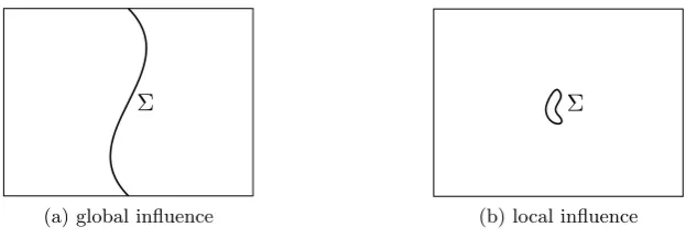
This certainly does not reflect the experience that the condition for random inputs is usually seen as unproblematic. An explanation for this codimension conundrum may be found in the simple illustration in Figure 1: although Σ does have codimension one in both pictures, it influences in the second case only a small part of the input space in this way; the predominant part of inputs perceives Σ as “smaller”.
Σ
(a) global influence
Σ
[image:4.595.141.458.313.421.2](b) local influence
Figure 1: Illustration of the possible influences of ill-posed inputs.
The result of such a situation is that the small part around the set of ill-posed inputs
dominates the complexity analysis. And this part of local points around Σ may in fact beexponentially small.
Remark 1.2. If one is only interested in the log of the condition, then this is not a big issue, and one may derive again general bounds for the expected condition of a slightly perturbed input, see [10] and [9, Ch. 22].
We adopt the setup of [10]: let Σ ⊆ Rn+1 be invariant under positive scaling and
let the condition number C: Sn → R be defined by C(x) = kxk/dist(x,Σ), where dist(x,Σ) = infy∈Σ{kx−yk}. Such a condition number is called a conic condition
number. For the smoothed analysis setting we denote for a pointz∈Snand σ >0 the ball, i.e., the spherical cap, in Sn of radiusσ aroundz byB(z, σ).
Theorem 1.3. Let Σ∩Sn ⊆W, where W 6=Sn is the zero set in Sn of homogeneous polynomials of degree at most d≥1 and let σ∈(0,1]. If codim Σ = 1 andz ∈Σ, then for x∈ B(z, σ) uniformly at random, E[C(x)] = ∞. On the other hand, regardless of the codimension, for all z ∈ Sn there exists a set Ez ⊆ Sn such that for x∈ B(z, σ) uniformly at random,
Prob{x∈Ez}< e−n, E
C(x)|x6∈Ez
< 13dn(n+ 1)
(1−e−n)σ =O dn2
σ
We note that the bounds in Theorem 1.3 are still rather coarse when applied in different settings, the reason being that they are quite general. For example, for a version κF(A) of the matrix condition number (using the Frobenius norm) we get from the above,
E[κF(A)|A6∈E] =O n4/σ
.
Once the derivation is understood, it is straight-forward to apply the weak average-case analysis to more precise, problem specific, bounds, such as the smoothed analysis of the matrix condition number by Wschebor [43].
1.2 Power iteration
Power iteration is a classic method for computing a dominant eigenvector and eigenvalue of a matrix. Let A∈Cn×n be a Hermitian matrix (this also works for other matrices, but for simplicity we restrict to this case) with eigenvaluesλi, ordered according to their absolute values, which are the singular values of the matrix,
|λ1| ≥ |λ2| ≥ · · · ≥ |λn|.
Letu1, . . . ,unbe eigenvectors corresponding to this ordering of eigenvalues. The eigen-valueλ1 is called a dominant eigenvalue, whileu1 is called a dominant eigenvector. The
power iteration generates a sequence of unit vectors pk,k≥0, by setting
pk =
Apk−1
kApk−1k
= A
kp
0
kAkp
0k
.
For a generic starting point, the algorithm converges geometrically with ratio |λ1|/|λ2|,
see [42, 9.2] or [25, 7.3] for an analysis. As there are degenerate cases in which the algorithm does not converge at all, or very slowly, it is natural to ask about the average-case complexity of power iteration, where the average is taken over both the starting points and the space of input matrices. Such an analysis was carried out by Kostlan [28, 29]. In [28], he analyzes the power method for matrices from the Gaussian orthogonal and unitary ensembles: the expected number of steps is infinite (Thm. 4.3); but in Thm. 4.4 he also proves a result akin to a weak average-case analysis, which he calls ‘generalized average’ (a notion he attributes to Smale), where he takes out a subset of the input space of measure η. Unfortunately, setting this measure exponentially small,
η = e−Ω(n), as required for a weak average-case analysis, only yields an exponential bound on the number of iterations. In [29], Kostlan discusses an iterated squaring method that understandably reduces the complexity of the method, but of course this is impractical for applications. The purpose of our work is to improve Kostlan’s analysis by showing that power iteration has polynomial weak average running time.
To quantify the convergence, we use the Fubini-Study metric (a.k.a. angle)
dR(x,y) = arccos
|hx,yi| kxkkyk
,
wherek · kis the norm induced by the Hermitian inner product onCn. For 0< α≤π/2 and x ∈Cn, let ρ
α(A,x) be the minimum number of iterations of the power method withp0 =xthat bring pk into an α-neighbourhood ofu1,
Define the expected value
ρα(A) = E
x∼U(CPn−1)
[ρα(A,x)],
where U(CPn−1) denotes the uniform distribution on complex projective space (the
notionρα(A,x) is well-defined onCPn−1). In what follows, we assume as random model
the Gaussian Unitary Ensemble (GUE). A GUE matrix is defined by H = 12(G+G∗), whereGis a complex Gaussian matrix, whose entries have standard Gaussian real and imaginary parts. In particular, the off-diagonal entries have real and imaginary part with mean 0 and variance 1/2, while the diagonal entries are real with mean 0 and variance 1.
Theorem 1.4. Let α ∈ (0, π/4), n ≥ 1, and H ∈ Cn×n a GUE matrix. Then there
exists a set En⊂Cn×n of exceptional inputs, such that Prob{H ∈En} ≤e−n,
and
E[ρα(H)|H 6∈En]<
p(n)
1−e−cn log cotα, p(n) =O(n
2)
for some constant c >0. In particular, power iteration runs in weak polynomial time.
The result rests on the analysis of the quotient of the largest two singular values of a GUE matrix. It would be interesting to see to what extent this result generalizes to other random models. The results are likely to carry over to Wigner matrices with sub-Gaussian entries. In this setting, the task would amount to finding good small ball probability bounds on the ratio or sum of extreme eigenvalues. A more challenging, though also more practically relevant, problem would be to study the ratio of singular values for a stochastic model of sparse and structured matrices, such as those that might arise in the discretisation of partial differential equations with random coefficients.
1.3 Renegar’s condition number and biconic feasibility
The primal and dual (homogeneous) feasibility problems with reference cone C ⊆ Rm are the decision problems
∃x∈C\ {0} s.t. Ax=0, (P) ∃y∈Rn\ {0} s.t. −ATy∈C◦, (D) where A ∈ Rn×m and C◦ = {z ∈ Rm | hx,zi ≤ 0 for all x ∈ C} denotes the polar cone ofC (the problem is to determine whether an input Asatisfies (P) or (D), which is almost surely, that is, for generic A, a strict alternative). Special cases of interest in conic optimisation are whenC is the non-negative orthant (LP), the second-order cone (QP), or the cone of positive semidefinite matrices (SDP). Other cases of interest, that include compressive sensing, are when C is the descent cone of a convex regularizer, in which case (the negation of) (P) is referred to as a nullspace condition.
also [9, 9.4]) that the number of iterations of a barrier method for solving the feasibility problem is bounded by O(√νC log(νC · RC(A))), where νC is the barrier parameter of C. Renegar’s condition numberRC(A) for descent cones of convex regularizers also appears uncredited in the error analysis of robust convex regularisation approaches to solving linear inverse problems [11, 23].
The condition number RC(A) can become arbitrary large as A approaches the boundary between (P) and (D). A probabilistic analysis of RC(A) and related quanti-ties has been carried out in various settings; a cone-independent result from [1] gives a bound of orderO(log(n)) for the expected logarithm of the related Grassmann condition number of a Gaussian matrix.
The theoretical bounds are somewhat out of sync with the observed performance. In fact, for largemandnand randomA, it turns out that one of (P) or (D) will hold with overwhelming probability, while the other will hold with negligible probability, rendering the feasibility problem almost trivial; see [3] and the references therein for a discussion of the associated phase transition phenomenon. One setting where this phenomenon has been embraced is compressive sensing [23] and its generalisations. In this framework, the dual feasibility (D) is equivalent to a convex relaxation being successful. From a more practical point of view, popular semidefinite programming solvers such as SDPT3 and Mosek rarely take more than 30 iterations on benchmark problems of various sizes [24, 16]; see also [34] for some experiments in the context of compressive sensing.
For symmetry reasons and to emphasise parallels to the matrix condition case, we consider in our analysis the following more general biconic convex feasibility problem with two nonzero closed convex cones C⊆Rm,D⊆Rn:
∃x∈C\ {0} s.t. Ax∈D◦, (P’) ∃y∈D\ {0} s.t. −ATy∈C◦. (D’) (A generalisation of) Renegar’s condition number is then defined by
RC,D(A) = min k
Ak
σC→D(A)
, kAk σD→C(−AT)
, (1)
where the smallest restricted singular value is defined as
σC→D(A) = min
x∈C∩Sm−1kΠD(Ax)k, ΠD(y) = min{ky−y
0k |y0 ∈D}.
Note that in the caseC=Rm,D=Rnwe recover the classical matrix condition number
RRm,Rn(A) =κ(A) =kAk kA†k,
where A† is the Moore-Penrose pseudoinverse of A. In this unrestricted case a lot is known about the distribution of the condition number for Gaussian matrices but also for more general ensembles [12, 35, 8, 36]; see [9, Notes to Ch. 4] for a concise discussion of this case. We only mention here that for Gaussian matrices it is known that ifmk, nk are such that limk→∞mk/nk =γ2, 0< γ <1, then
RRm,Rn(G) =κ(G)→
1 +γ
1−γ almost surely.
In particular, in this asymptotic setting the expected condition number is of constant
order.
such that their “formats” satisfy similar asymptotics as above, then we will show that Renegar’s condition number does indeed have constant weak average-case complexity. We will describe next what we mean by similar format, after introducing a notion of dimension of a closed convex cone.
The statistical dimension of a closed convex coneC⊆Rm may be characterized as
δ(C) = E
g∼N(0,Im)
kΠC(g)k2
.
It coincides with the usual dimension ifCis the full space,δ(Rm) =m. We now consider families of conesCk⊆Rmk,Dk⊆Rnk, and we assume that we have the asymptotics
lim k→∞
δ(Ck)
mk
=α2, lim k→∞
δ(Dk)
nk
=β2, lim k→∞
mk
nk
=γ2 (2)
with 0 < α, β, γ ≤ 1. A typical example for this situation is Ck ⊆ Rmk self-dual and
Dk=Rnk, in which case δ(Ck) = m2k and δ(Dk) = nk, so thatα = √12 and β = 1. We will assume that β 6= αγ, and since RC,D(A) =RD,C(−AT), we may assume without loss of generality
β > α γ. (3)
Closely related, but conceptually different, to the statistical dimension is the Gaus-sian width of a cone,w(C) = E
g∼N(0,Im)
kΠC(g)k
(actually, it is the Gaussian width of
the intersection with the unit ball C∩Bn, but we adopt a purely conic point of view here). The squared Gaussian width w2(C) differs from the statistical dimension by at most one [3, Prop. 10.2],w2(C)≤δ(C)≤w2(C) + 1. In particular, the asymptotics (2) hold for the squared Gaussian width if and only if they hold for the statistical dimension.
Theorem 1.5. If Ck⊆Rmk, Dk⊆Rnk are families of cones such that the dimensions
satisfy the asymptotics (2) with β > αγ, and nk → ∞ for k → ∞, then there exist
exceptional sets Ek with Prob{G∈Ek} ≤e−Ω(nk), such that
E[RC,D(G)|G6∈Ek]< uk(C, D), uk(Ck, Dk)→ 1 +γ β−αγ.
In particular, if nk= Ω(k), then the weak average-case complexity of RC,D is constant. The probabilistic analysis of Renegar’s condition number for arbitrary cones has so far been confined to [1] (though there has been considerable work on the linear programming case, see [9] and the references therein). These results were obtained following the classical tail estimate approach. The new approach of allowing to ignore exponentially small input sets, which loosens the requirements for the tail bounds so that for fixed dimensions we do not even require the bounds to go to zero, opens up new ways to directly exploit concentration of measure phenomena. We will do this through the use of Gordon’s escape-through-the-mesh approach [26, 17].
1.4 Relation to previous work
given to practically impossible events. An overview of previous work in the probabilistic analysis of numerical algorithms via condition numbers, that includes smoothed analysis and much more, can be found in [9].
The point of view of weak average-case analysis is not unusual in the setting of non-asymptotic random matrix theory [40] and its applications, such as compressive sensing and related fields [23]. Rather than focussing on precise tail bounds Prob{X > t} that decay to zero for fixed nast→ ∞, and the associated expected values, the emphasis is on showing that a quantity of interest is confined to a certain region with overwhelming probability. In the setting of complexity theory this point of view seems to be new.
We would also like to point out that the idea of removing “bad cases” from a prob-abilistic analysis has featured in other probprob-abilistic settings [38, 13, 14, 15, 19].
1.5 Organisation of paper
The remaining sections are devoted to the proofs of the three main results, Theo-rems 1.3, 1.4 and 1.5. Section 2 deals with the easiest case, condition numbers inversely proportional to a set of ill-posed inputs. Here, a weak average-case analysis follows in a straight-forward way from a simple probabilistic observation on the effect of condition-ing out large deviations from an expectation. Section 3 deals with the power iteration. For convenience, we recreate Kostlan’s derivation of the number of iterations needed to approach a dominant eigenvector in terms of the ratio of the largest singular values. The probabilistic analysis and proof of Theorem 1.4 then follows from known results on random matrices from the Gaussian unitary ensemble. Finally, Section 4 presents some basic facts about the biconic feasibility problem and Gordon’s inequalities (discussed in more depth in [2]), followed by the proof of Theorem 1.5
1.6 Acknowledgments
The authors would like to thank Felipe Cucker for encouragement and useful comments on a preliminary draft.
2
Conic condition numbers
We begin with some basic probabilistic observations about the effect of conditioning on the expectation of a quantity such as a condition number. We also include the weak average-case analysis of conic condition numbers, since it is a trivial consequence of Lemma 2.2. The first observation is that for a weak average-case analysis of a random variable X, while we are allowed to remove any small enough set from the probability space, we do best by removing a set of the form {X > t}. Therefore, weak average-case analysis ofXis equivalent to an average-case analysis of a truncationX≤t:=X·1{X ≤
t} for a suitable parametert >0.
Lemma 2.1. Let (Ω,F, µ) be a probability space and X a random variable that is absolutely continuous with respect toµ. Givenε >0, lettbe such thatProb{X > t}=ε. Then for any measurable S⊂Ωwith µ(S)≤ε,
E
X |X≤t≤E
X|S.
{ω ∈ S | X(ω) ≤ t} and S>t = {ω ∈ S | X(ω) > t}. Then we have the disjoint decompositionsS =S≤t∪S>t and
{ω∈Ω|X(ω)≤t}=S≤t∪ {ω∈S|X(ω)≤t}. Since Prob{X≤t}= 1−ε=µ(S), we get
µ(S>t) =µ({ω∈S|X(ω)≤t}). (4) For the conditional probabilities we obtain
E
X|X≤t
= 1
1−ε
Z
S≤t
X(ω)dµ+ Z
{S|X(ω)≤t}
X(ω)dµ
≤ 1
1−ε
Z
S≤t
X(ω)dµ+tµ({S|X(ω)≤t})
(4)
= 1
1−ε
Z
S≤t
X(ω)dµ+tµ(S>t)
≤ 1
1−ε
Z
S
X(ω)dµ=E
X|S
.
The next lemma shows how to get finite conditional expectations from tail bounds of order t−1. This will be key for the weak average-case analysis of conic condition numbers and the power iteration method.
Lemma 2.2. Let X be a non-negative random variable on a probability space (Ω,F, µ)
such that for some a >0 and for all t > a,
Prob{X > t} ≤ a
t. (5)
Then, for t > a,
E
X|X ≤t
≤ a
1−a t
1−loga
t
.
Proof. The proof is a straight-forward calculation:
E
X |X≤t
= 1
1−Prob{X > t}
Z t
0
Prob{X > s} ds
≤ 1
1−at
a+ Z t
a
Prob{X > s} ds
≤ a
1−at(1 + log(t)−log(a)).
LetC(x) be a conic condition number as specified in Theorem 1.3. In [10, Thm. 1.1] it is shown that for this kind of condition numbers,
Prob
x∈B(z,σ)
{C(x)> t}< 13dn
tσ ift≥(1 + 2d)(n−1)/σ. (6)
Combining this powerful result with the simple Lemma 2.2 yields Theorem 1.3.
Proof of Theorem 1.3. Set a := 13σdn. Since a= 13dn/σ > (1 + 2d)(n−1)/σ, the tail bound (6) holds in particular for t≥a. SettingEn={x| C(x)> aen}, we obtain
Prob
x∈B(z,σ)
{x∈En}< e−n.
Therefore,
E
x∈B(z,σ)
C(x)|x6∈En
= E
x∈B(z,σ)
C(x)| C(x)≤aenLem. 2≤ .2 a(n+ 1)
1−e−n =
13dn(n+ 1) (1−e−n)σ .
3
Power iteration
We first review a bound on the number of iterations needed to get within a certain distance of the dominant eigenvector. We use the notation from Section 1.2. Recall that for 0< α≤π/2 andx∈Cn,ρ
α(A,x) denotes the minimum number of iterations that bring Akxinto an α-neighbourhood ofu1,
ρα(A,x) = min{k|dR(pk,u1)≤α},
and the expected value is defined as
ρα(A) = E
x∼U(CPn−1)
[ρα(A,x)],
where U(CPn−1) denotes the uniform distribution on complex projective space. For a
linear subspaceL⊆Cn, writeΠ
L(x) = argminy∈Lky−xkfor the projection ofxontoL, and letΠi(x) :=Πspan{ui}(x) be the projection onto the linear subspace spanned by the
i-th eigenvector. The following result can be found in a slightly modified form in [28]; the proof is a variation of the well-known analysis of the power method in terms of the ratio of largest singular values, see for example [42, 9.2] or [25, 7.3]. For convenience we provide a complete derivation of the starting point dependent results, since the proof in [28] is rather sketchy.
Theorem 3.1 (Kostlan [28]). Assume x∈Cn is not orthogonal to the dominant
eigen-vector u1 of A, |hx,u1i|< π2. Then
ρα(A,x)≥
log cot(α) + logkΠ2(x)k −logkΠ1(x)k
log|λ1| −log|λ2|
and
ρα(A,x)≤
log cot(α) + logkΠu⊥
1(x)k −logkΠ1(x)k log|λ1| −log|λ2|
.
The expected number of steps is bounded by
log cot(α) log|λ1| −log|λ2|
≤ρα(A)≤
1
2(log(n) + 2
n−1
n ) + max{0,log cotα} log|λ1| −log|λ2|
.
Proof. Assume kxk = 1 and write x = a1u1 +· · ·+anun. Then, in particular, a1 =
kΠ1(x)k,a2=kΠ2(x)k, and a2u2+· · ·+anun=Πu⊥
1(x). Note that for any k≥1,
Akx=a1λk1u1+· · ·+anλknun. Let k=ρα(A,x) be the smallest integer such that
cos(α)≤ |hA
kx,u
1i|
kAkxk =
|a1λk1|
kAkxk =
kΠ1(x)k|λ1|k
kAkxk . (7)
From the identity sin2(α) + cos2(α) = 1 we obtain
sin(α)≥
p
a22|λ2|2k+· · ·+a2n|λn|2k
kAkxk ≥
|λ2|kkΠ2(x)k
Putting (7) and (8) together, we get
cot(α)≤
|
λ1|
|λ2|
k k
Π1(x)k
kΠ2(x)k
⇒ k≥ log cot(α) + logkΠ2(x)k −logkΠ1(x)k
log|λ1| −log|λ2|
.
This shows the first inequality. For the second inequality, let k < ρα(A,x). Then after
k iterations we are still outside anα neighbourhood of u1, so that
cos(α)≥ |hA
kx,u
1i|
kAkxk =
|a1λk1|
kAkxk =
kΠ1(x)k|λ1|k
kAkxk . (9)
Similar as in (8), we get
sin(α)≤
p
a2
2|λ2|2k+· · ·+a2n|λn|2k
kAkxk ≤
|λ2|kkΠu⊥
1(x)k
kAkxk . (10)
Combining (9) and (10) gives
cot(α)≥
|λ1|
|λ2|
k
kΠ1(x)k
kΠu⊥
1 (x)k
⇒ k≤ log cot(α) + logkΠu
⊥
1(x)k −logkΠ1(x)k log|λ1| −log|λ2|
,
which establishes the second inequality.
For the expected values of the bounds we refer to Kostlan’s work [28].
3.1 Weak average-case analysis of power iteration
Theorem 3.1 implies that the relevant probability in the average-case analysis of power iteration is
Prob
1
log|λ1| −log|λ2|
> x
= Prob |
λ1|
|λ2|
< e1x
.
Letλmax,λ2max,λmin andλ2mindenote the largest, second largest, smallest and second
smallest eigenvalue of a GUE matrix H, respectively. Keep in mind that this refers to the eigenvalues themselves, not their absolute values, which underlie the ordering
|λ1| ≥ · · · ≥ |λn|. Before proceeding, we collect some known results on the distribution of the eigenvalues of a GUE matrix. To ease notation, in what follows,C andcare used for absolute constants which may change from line to line.
1. The probability that all eigenvalues are positive (or all are negative) is exponen-tially small [18],
Prob{λmin>0} ≤Ce−cn
2
(11)
for some constants C and c.
2. The largest eigenvalue of a GUE matrix satisfies
Prob{λmax≥
√
n(2 +ε)} ≤Ce−cnε3/2 (12) for some constantsCandc(e.g., [30, Prop. 2.1], note the slightly different form). We will use this with ε= 1.
3. The smallest gap δmin between consecutive eigenvalues satisfies
Prob{δmin≤δ/
√
Proof of Theorem 1.4. Assume x ≥1. Throughout the proof, we will use the fact that
−λmin and λmax have the same distribution, as well as −λ2min and λ2max. For the
relationship between the singular values and the eigenvalues we have the following two cases:
1. The largest and second largest singular values come from the two largest or from the two smallest eigenvalues, that is,λ1 =λmaxandλ2=λ2max, orλ1=λmin and
λ2=λ2min.
2. The largest and second largest singular values come from the largest (positive) and smallest (negative) eigenvalues, that is, λ1 = λmax and λ2 = λmin, orλ1 = λmin
and λ2 =λmax.
Using the union bound we may consider these cases separately:
Prob |
λ1|
|λ2|
< e1x
≤Prob
|
λmax|
|λ2max|
< e1x
+ Prob |
λmin|
|λ2min|
< ex1
+ Prob
e−1x < |λmax|
|λmin|
< e1x
Clearly, the first two terms on the right-hand side are subject to the same analysis. Adjacent eigenvalues. We consider the case where the largest and second largest singular values are the largest and second largest (positive) eigenvalues of the matrix. Note that for x ≥1 we havee1/x−1<2/x, which will be used in the sequel. We will also generically useC andcfor constants that may vary within one derivation. We have forx≥1,
Prob |
λmax|
|λ2max|
< ex1
≤Prob
λmax
λ2max
< ex1
= Prob
λmax−λ2max
λ2max
< e1/x−1 ≤Prob δmin λmax < 2 x
(12),ε=1
≤ Prob
δmin<
6n x√n
+Ce−cn
(13)
< 216n
4
x3 +Ce
−cn.
For x >6n4/3 and nlarge enough, the bound becomes non-trivial.
Extreme eigenvalues. For the ratio of the eigenvalues at the edge we have forx≥1,
Prob
e−1x < |λmax|
|λmin|
< e1x
≤Prob
e−1x < λmax
−λmin
< e1x
+ 2 Prob{λmin >0}
(11)
≤ Prob
λmax
−λmin
< e1x
−Prob
λmax
−λmin
≤e−x1
+Ce−cn2
= Prob
λmax
−λmin
< e1x
−
1−Prob
λmax
−λmin
> e−1x
+Ce−cn2
= 2 Prob
λmax
−λmin
< e1x
−1 +Ce−cn2
= 2 Prob
λmax+λmin
−λmin
< e1x −1
−1 +Ce−cn2
≤2 Prob
λmax+λmin
−λmin
< 2 x
−1 +Ce−cn2
(12),ε=1
≤ 2 Prob
λmax+λmin<
6√n x
Sinceλmaxand−λminare equally distributed, the differenceλmax−(−λmin) is symmetric
around the origin, so that we obtain
2 Prob
λmax+λmin<
6√n x
−1 = Prob
−6
x < λ√max
n + λ√min
n <
6
x
.
Now consider the normalized variables
˜
λmax:=n2/3
λmax
√
n −2
, ˜λmin :=n2/3
λmax
√
n + 2
.
The maximumM of the density of ˜λmax+ ˜λmin is bounded, as can be deduced directly
from the joint distribution of the eigenvalues of the GUE ensemble. We thus obtain
Prob
− 6n
2/3
x <λ˜max+ ˜λmin <
6n2/3 x
≤ 12M n
2/3
x .
In summary, we have the bound
Prob
e−1x < |λmax|
|λmin|
≤ex1
≤ 12M n
2/3
x +Ce
−cn. (14)
Combined bound. Putting the bounds together, we get
Prob
1
log|λ1| −log|λ2|
> x
< 12M n
2/3
x +
432n4 x3 +Ce
−cn
for some constantK. This bound is non-trivial forx > Kn4/3 for a suitable constantK. Setx0=Kn4/3ecn and
En:= H 1
log|λ1| −log|λ2|
> x0
.
Then
Prob{H ∈En}< Ce−cn
for suitable absolute constants C and c. We can apply a variation of the proof of Lemma 2.2 (with an adjustment to take into account thex−3and the exponential term), witha=Kn4/3 and t=x0, to get
E
h
(log|λ1| −log|λ2|)−1
En i < Kn 2
1−e−cn
for some absolute constant K. Incorporating the numerator from the bound on the
power iteration gives the desired result.
Remark 3.2. With a more careful analysis, the constants in the bounds can be explicitly estimated, but we haven’t done so as the first aim was to establish a polynomial bound.
4
Renegar’s condition number
Note that we have a complete symmetry between (P’) and (D’) via the exchange of A
by−AT and by a swap betweenCandD. We denote the set of primal feasible instances and the set of dual feasible instances by
P(C, D) :={A∈Rn×m |(P’) is feasible}, D(C, D) :={A∈Rn×m |(D’) is feasible},
and we call
Σ(C, D) :=P(C, D)∩ D(C, D)
the set of ill-posed inputs. Indeed, it can be shown that P(C, D) and D(C, D) are both closed, the union of P(C, D) andD(C, D) is the whole input space Rn×m unless
C = D = Rm, and the probability that a Gaussian matrix lies in Σ(C, D) is zero [2, Sec. 2.2].
As for the relation of this generalized feasibility problem to conically restricted linear operators, observe that A∈ P(C, D) if and only if σC→D(A) = 0, and A∈ D(C, D) if and only if σD→C(−AT) = 0. Moreover, we have [2, Sec. 2.2]
dist(A,P) =σC→D(A), dist(A,D) =σD→C(−AT), (15) where dist denotes the Euclidean distance.
The following theorem is the consequence of a classic result by Gordon [26]. For various derivations, see [17, 23]. The form stated here, for a map between two cones, is from [2]. Here, we use the Gaussian widthw(C) = E
g∼N(0,Im)
kΠC(g)k
.
Theorem 4.1. Let C ⊆ Rm, D ⊆ Rn closed convex cones, and let G ∈ Rn×m be a
Gaussian matrix. Then for λ≥0,
ProbkGkC→D ≥w(C) +w(D) +λ ≤e−
λ2
2 ,
Prob
σC→D(G)≤w(D)−w(C)−λ ≤e−
λ2
2 . (16)
Before getting to the proof of the asymptotic statement in Theorem 1.5 we use Gordon’s estimate (16) for the following finite-dimensional bound.
Proposition 4.2. LetC⊆Rm,D⊆Rnclosed convex cones withw(D)−w(C)>2√2,
and let G ∈ Rn×m be a Gaussian matrix. Then there exists a set E ⊆ Rn×m with Prob{G∈E}< ε:= 2e−(w(D)−w(C))2/8, such that
E[RC,D(G)|G6∈E]< 1 1−ε
w(Rn) +w(Rm)
w(D)−w(C) + 4 Z a+b
2a
b a
e−(as−b2 )2 (1−s)2 ds
, (17)
where a= 12 w(Rm) +w(Rn) +w(D)−w(C)
, b= 12 w(Rm) +w(Rn)−(w(D)−w(C)
.
Proof. To ease the notation, setwm =w(Rm),wn=w(Rn). Note thata+b=wm+wn and a−b = w(D) −w(C). Equations (16) and the union bound give for 0 ≤ λ < w(D)−w(C),
Prob k
Gk
σC→D(G)
≥ wm+wn+λ
w(D)−w(C)−λ
≤2e−λ
We introducet= wm+wn+λ
w(D)−w(C)−λ, for which t−1
t+1 =
b+λ
a , so that we can rewrite the bound as
Prob
kGk
σC→D(G)
≥t
≤2 exp
−1
2
at−1 t+ 1−b
2
.
This holds for tt−+11 ≥ b
a, or equivalently, t ≥ a+b a−b =
wm+wn
w(D)−w(C). In particular, for
tε:= 2aa+−bb + 1, that is, tε−1
tε+1 =
a+b
2a , we have
Prob k
Gk
σC→D(G)
≥tε
≤2 exp− (a−b)
2
8
=ε.
Defining the exceptional set E := {G | σ kGk
C→D(G) ≥ tε}, we have, in particular, that
σC→D(G) > 0 for G6∈ E. By (1) and (15) this implies that the condition number of
G6∈Eis given byRC,D(G) = σC→DkGk(G). For the conditional expectation we thus obtain
E[RC,D(G)|G6∈E]≤ 1 1−ε
Z tε 0
Prob n
RC,D(G)≥tand G6∈E o
dt
≤ 1
1−ε
a+b a−b+ 2
Z tε a+b a−b
exp−1
2
at−1 t+ 1−b
2
dt
.
Substituting s= tt−+11, the expression reads as
E[RC,D(G)|G6∈E]≤ 1
1−ε
a+b a−b+ 4
Z a+b 2a
b a
e−(as−b2 )2 (1−s)2 ds
,
which was to be shown.
For the proof of Theorem 1.5 it remains to estimate the integral in (17). Since the boundaries of integration are both in the interval (0,1) we could get an easy bound by computing the maximum of the integrand and bounding the integral accordingly. Instead, we will use Laplace’s method [4] to show that the integral goes to zero in the assumed asymptotic setting.
Proof of Theorem 1.5. Recall that Ck ⊆ Rmk, Dk ⊆ Rnk are families of cones such that the dimensions satisfy limk→∞δ(Ck)/mk = α2, limk→∞δ(Dk)/nk = β2, and limk→∞mk/nk =γ2, with 0 < α, β, γ ≤ 1 and β > α γ. To see that Proposition 4.2, applied to these sequences of cones, does indeed give the claimed asymptotics in Theo-rem 1.5, note first that the size of the exceptional set is bounded by e−Ω(nk), as
(w(D)−w(C))2
nk
= w(D)
2
nk
−2w(D)w(C)
nk
+w(C)
2
nk
→β2−2αβγ+αγ =β(β−αγ) +αγ(1−β)>0,
where we usedw(C)2 ≤δ(C)≤w(C)2+ 1 and the assumptionnk→ ∞ fork→ ∞. So the size of the exceptional set is small enough.
Hence, all that remains to show is that the integral in the bound (17) goes to zero fork→ ∞. More precisely, if we define as in Proposition 4.2,
ak = w(R
mk)+w(Rnk)
2 +
w(Dk)−w(Ck)
2 , bk =
w(Rmk)+w(Rnk)
2 −
w(Dk)−w(Ck)
then the decisive term from (17) is given by
Rk:=
Z ak2+bk
ak
bk ak
g(s) exp nkfk(s)
ds,
where g(s) = (1−s)−2 and fk(s) =−(aks
−bk)2
2nk , which we need to show that it goes to
zero.
The lower integral bound is not a problem so that we use the trivial lower bound
bk/ak≥0. For the upper integral bound we have the asymptotics
ak+bk 2ak
= w(R
mk) +w(Rnk)
w(Rmk) +w(Rnk) +w(Dk)−w(Ck) →u:=
1
1 +β1++αγγ <1, and for the functions fk we notice that
fk(s) =−
w(Rmk) nk +
w(Rnk)
nk
(s−1) + w(Dk)
nk −
w(Ck)
nk
(s+ 1)2
8
→f(s) :=−((γ+ 1)(s−1) + (β−αγ)(s+ 1))
2
8 .
So if we define
R:= Z u
0
g(s)enf(s)ds,
we see that all that remains is to show thatR→0 forn→ ∞. Now,f(s) can be written in the form
f(s) =−(cs−d)
2
8 , c=γ+ 1 +β−αγ, d=γ+ 1−(β−αγ),
and we can estimate R≤g(u) Ru
0 e
−n(cs−d)2/8
ds. Since
0< d c =
γ+ 1−(β−αγ)
γ+ 1 +β−αγ <
γ+ 1
γ+ 1 +β−αγ =u,
Laplace’s method yields R0ue−n(cs−d)2/8ds= O(n−1/2). This shows R → 0 for n→ ∞
and thus finishes the proof.
References
[1] D. Amelunxen and P. B¨urgisser. Probabilistic analysis of the Grassmann condition number. Found. Comput. Math., 15(1):3–51, 2015.
[2] D. Amelunxen and M. Lotz. Gordon’s inequality and condition numbers in conic optimization. arXiv:1408.3016 [math.PR].
[3] D. Amelunxen, M. Lotz, M. B. McCoy, and J. A. Tropp. Living on the edge: phase transitions in convex programs with random data. Inf. Inference, 3(3):224–294, 2014.
[5] P. Bianchi, M. Debbah, and J. Najim. Asymptotic independence in the spectrum of the Gaussian unitary ensemble. Electron. Commun. Probab, 15:376–395, 2010.
[6] F. Bornemann. Asymptotic independence of the extreme eigenvalues of Gaussian unitary ensemble. Journal of Mathematical Physics, 51(2):023514, 2010.
[7] P. B¨urgisser. Smoothed analysis of condition numbers. In Proceedings of the In-ternational Congress of Mathematicians, Hyderabad, volume IV, pages 2609–2633. World Scientific, 2010.
[8] P. B¨urgisser and F. Cucker. Smoothed analysis of Moore–Penrose Inversion. SIAM Journal on Matrix Analysis and Applications, 31(5):2769–2783, 2010.
[9] P. B¨urgisser and F. Cucker. Condition: The geometry of numerical algorithms. Number 349 in Grundlehren der Mathematischen Wissenschaften. Springer Verlag, 2013.
[10] P. B¨urgisser, F. Cucker, and M. Lotz. The probability that a slightly perturbed numerical analysis problem is difficult. Math. Comp., 77(263):1559–1583, 2008.
[11] V. Chandrasekaran, B. Recht, P. A. Parrilo, and A. S. Willsky. The convex geometry of linear inverse problems. Found. Comput. Math., 12(6):805–849, 2012.
[12] Z. Chen and J. J. Dongarra. Condition numbers of Gaussian random matrices.
SIAM J. Matrix Anal. Appl., 27(3):603–620 (electronic), 2005.
[13] A. Coja-Oghlan. The asymptotic k-sat threshold. InProceedings of the 46th Annual ACM Symposium on Theory of Computing, pages 804–813. ACM, 2014.
[14] A. Coja-Oghlan and D. Vilenchik. Chasing the k-colorability threshold. In Founda-tions of Computer Science (FOCS), 2013 IEEE 54th Annual Symposium on, pages 380–389. IEEE, 2013.
[15] A. Coja-Oghlan and L. Zdeborov´a. The condensation transition in random hyper-graph 2-coloring. InProceedings of the twenty-third annual ACM-SIAM symposium on Discrete Algorithms, pages 241–250. SIAM, 2012.
[16] J. Dahl. Semidefinite optimization using MOSEK. ISMP, Berlin, 2012.
[17] K. R. Davidson and S. J. Szarek. Local operator theory, random matrices and Banach spaces. Handbook of the geometry of Banach spaces, 1:317–366, 2001.
[18] D. S. Dean and S. N. Majumdar. Extreme value statistics of eigenvalues of Gaussian random matrices. Phys. Rev. E (3), 77(4):041108, 12, 2008.
[19] V. Diekert, A. G. Myasnikov, and A. Weiß. Amenability of Schreier graphs and strongly generic algorithms for the conjugacy problem. arXiv:1501.05579 [math.GR].
[20] A. Edelman and M. La Croix. The singular values of the GUE (less is more). arXiv:1410.7065 [math.PR].
[22] L. Erd˝os, B. Schlein, and H.-T. Yau. Wegner estimate and level repulsion for Wigner random matrices. International Mathematics Research Notices, 2010(3):436–479, 2010.
[23] S. Foucart and H. Rauhut. A mathematical introduction to compressive sensing, volume 336 ofApplied and Numerical Harmonic Analysis. Birkh¨auser, Basel, 2013.
[24] R. M. Freund, F. Ord´o˜nez, and K.-C. Toh. Behavioral measures and their corre-lation with IPM iteration counts on semi-definite programming problems. Mathe-matical programming, 109(2-3):445–475, 2007.
[25] G. Golub and C. Van Loan. Matrix computations. Johns Hopkins Studies in the Mathematical Sciences. Johns Hopkins University Press, Baltimore, MD, third edi-tion, 1996.
[26] Y. Gordon. On Milman’s inequality and random subspaces which escape through a mesh inRn. In Geometric aspects of functional analysis (1986/87), volume 1317 ofLecture Notes in Math., pages 84–106. Springer, Berlin, 1988.
[27] I. M. Johnstone and Z. Ma. Fast approach to the Tracy-Widom law at the edge of GOE and GUE. The Annals of Applied Arobability: an official journal of the Institute of Mathematical Statistics, 22(5):1962, 2012.
[28] E. Kostlan. Complexity theory of numerical linear algebra.J. Comput. Appl. Math., 22(2-3):219–230, 1988. Special issue on emerging paradigms in applied mathemat-ical modelling.
[29] E. Kostlan. Statistical complexity of dominant eigenvector calculation. J. Com-plexity, 7(4):371–379, 1991.
[30] M. Ledoux. Deviation inequalities on largest eigenvalues. In Geometric aspects of functional analysis, pages 167–219. Springer, 2007.
[31] H. Nguyen, T. Tao, and V. Vu. Random matrices: tail bounds for gaps between eigenvalues. arXiv:1504.00396 [math.PR].
[32] J. Renegar. Some perturbation theory for linear programming.Math. Programming, 65(1, Ser. A):73–91, 1994.
[33] J. Renegar. Linear programming, complexity theory and elementary functional analysis. Math. Programming, 70(3, Ser. A):279–351, 1995.
[34] V. Roulet, N. Boumal, and A. d’Aspremont. Renegar’s condition number and compressed sensing performance. arXiv:1506.03295 [math.PR].
[35] M. Rudelson and R. Vershynin. Smallest singular value of a random rectangular matrix. Comm. Pure Appl. Math., 62(12):1707–1739, 2009.
[37] D. A. Spielman and S.-H. Teng. Smoothed analysis of algorithms and heuristics: progress and open questions. InFoundations of computational mathematics, San-tander 2005, volume 331 of London Math. Soc. Lecture Note Ser., pages 274–342. Cambridge Univ. Press, Cambridge, 2006.
[38] R. Venkataramanan and S. Tatikonda. The Gaussian rate-distortion function of sparse regression codes with optimal encoding. In Information Theory (ISIT), 2014 IEEE International Symposium on, pages 2844–2848. IEEE, 2014.
[39] J. C. Vera, J. C. Rivera, J. Pe˜na, and Y. Hui. A primal-dual symmetric relaxation for homogeneous conic systems. J. Complexity, 23(2):245–261, 2007.
[40] R. Vershynin. Introduction to the non-asymptotic analysis of random matrices. In Y. C. Eldar and G. Kutyniok, editors, Compressed sensing, pages xii+544. Cam-bridge University Press, CamCam-bridge, 2012. Theory and applications.
[41] J. von Neumann and A. H. Taub. John von Neumann Collected Works: Volume V - Design of Computers, Theory of Automata and Numerical Analysis.
[42] J. H. Wilkinson. The algebraic eigenvalue problem. Clarendon Press, Oxford, 1965.